Relativistic Generalization of the Gamow Factor
for Fermion Pair Production or Annihilation

Abstract

In the production or annihilation of a pair of fermions, the initial-state or final-state interactions often lead to significant effects on the reaction cross sections. For Coulomb-type interactions, the Gamow factor has been traditionally used to take into account these effects. However the Gamow factor needs to be modified when the magnitude of the coupling constant or the relative velocity of two particles increases. We obtain the relativistic generalization of the Gamow factor in terms of the overlap of the Feynman amplitude with the relativistic wave function of two fermions with an attractive Coulomb-type interaction. An explicit form of the corrective factor is presented for the spin-singlet S-wave state. While the corrective factor approaches the Gamow factor in the non-relativistic limit, we found that the Gamow factor significantly over-estimates the effects when the coupling constant or the velocity is large.

I Introduction

The final-state interaction (FSI) and initial-state interaction (ISI) are important processes in particle and nuclear physics Bet56 ; Gam28 ; Som39 ; Bar80 ; Gus88 ; Fad88 ; Fad90 ; Bro95 ; Cha95a ; Won96d ; Won97 ; Yoon00 ; Yoon03 . They lead to an enhancement of the reaction cross section for attractive interactions and a suppression for repulsive interactions. The effects are especially large near the production threshold in the region of low-energy annihilation. We shall describe these FSI/ISI in terms of a corrective factor which we shall call the $K$-factor. It is defined as the ratio of the cross section with the interaction to the corresponding quantity without the interaction.

In non-relativistic physics the $K$-factor can be obtained by solving the two-body Schrödinger equation nonperturbatively under their mutual interaction. It is determined by calculating the absolute square of the relative wave function at the origin. As is well known, for the electric-Coulomb and color-Coulomb interaction, $V(r)=-\alpha/r$, the non-relativistic corrective $K$-factor is the Gamow-Sommerfeld factor Gam28 ; Som39 (or simply called, the Gamow factor),

$$G(\eta)={2\pi\eta\over 1-e^{-2\pi\eta}},$$ (1)

where $\eta$ is the Sommerfeld parameter,

$$\eta={\alpha\over v},$$ (2)

$\alpha$ is the coupling constant (positive for an attractive Coulombic interaction), and $v$ is the relative velocity of two particles. For two-equal masses which we shall consider in this paper, $v$ is given in terms of their center-of-mass energy $\sqrt{s}$ by Yoon00 ; Tod71 ; Cra91 ,

$$v={(s^{2}-4sm^{2})^{1/2}\over s-2m^{2}}.$$ (3)

This gives $v\sim 2\sqrt{1-4m^{2}/s}$ when $\sqrt{s}\sim 2m$ and $v\rightarrow 1$ when $s\rightarrow\infty$.

As was pointed out by Chatterjee and her collaborator Cha95a ; Won96d ; Won97 , the Gamow factor Eq. (1), has been traditionally used to study non-relativistic Coulomb-type ISI/FSI in reactions involving production or annihilation of particles. The results are then interpolated with the well-known perturbative QCD corrective $K$-factor at high energies, following the procedure of Schwinger Sch73 . It predicts an enhancement for $q\bar{q}$ in color-singlet states and a suppression for color-octet states, the effect increasing as the relative velocity decreases. Consequences on dilepton production in the quark-gluon plasma, the Drell-Yan process, and heavy quark production processes were also examined.

Although the above Gamow factor gives an approximate description of the FSI/ISI effects Cha95a , it is useful to obtain a more accurate description as there are physical processes in which the interaction coupling constant or the relative velocity of the pair can be quite large and the use of the non-relativistic treatment may not be adequate. For example, in the production of a charm quark pair, the coupling constant of the color-Coulomb interaction between the charm quark and antiquark is about $0.3$, which is quite large. Furthermore, as the charm quark mass is large, the magnitude of the relative velocity between the produced quark and antiquark can be quite small in low-energy production near the threshold. The FSI/ISI effects can be quite large for large coupling constants and small relative velocities. Baym and P. Braun-Munzinger modified the Gamow factor in their study of the final-state Coulomb interaction and effects on the Hanbury-Brown Twiss effects of intensity interferometry Bay96 . A negatively charged particle in a nucleus with a large $Z$ number will also be subject to strong FSI/ISI. Although the effect of the interaction is very large for low relative velocities, it is nonetheless useful to see how the effect varies as the velocity increases. For brevity of notation, we shall use the term “Coulomb interaction” with a variable coupling constant to refer to both the electric-Coulomb and color-Coulomb interactions. We shall limit our attention to attractive Coulomb interactions, although similar formulation can be carried out for repulsive Coulomb interactions and screened Yukawa interactions Cha95a ; Won96d ; Won97 .

Relativistic treatment is needed for strongly attractive interactions, even when the relative asymptotic velocity between two particles at $r\to\infty$ is small, as two particles can reach relativistic velocities at short distances due to the strongly attractive interaction. Relativistic treatment is also needed when the asymptotic relative velocity of two particle approaches the speed of light.

The evaluation of the relativistic corrective $K$-factor involves the non-perturbative treatment of the relativistic two-body equation of motion under their mutual interaction. Compared with the non-relativistic Schrödinger equation involving the Coulomb potential, there is an additional attractive effective potential proportional to $-|V(r)|^{2}$, and a repulsive term from the space-like part of the gauge interaction, which lead to a non-trivial behavior when the coupling constant becomes large. In the case of fermions with the Coulomb interaction, there are further modifications associated with additional spin-dependent potentials.

In a previous study Yoon00 we presented a method to study the relativistic Coulomb FSI/ISI effects for a pair of bosons. The corrective $K$-factor was evaluated by taking the overlap of the relativistic wave function with the corresponding Feynman amplitude. Its analytic form was obtained and its numerical values were compared with those of the Gamow factor. For attractive interactions, we found that the Gamow factor over-estimates the corrective factor for most energies and even more in the relativistic region with a large magnitude of the coupling constants.

We would like to generalize these previous boson results to a pair of fermions with an attractive Coulomb-type final state interaction. The fermion results are of more practical interest as the electromagnetic gauge field or the chromodynamical gauge field couples to fermion fields and the results obtained here may be directly applied to the production or annihilation of a pair of fermions in a color-singlet state. A brief report of the present results was presented in ref. Yoon03

II The $K$-factor

We shall be interested in processes involving the production or annihilation of a pair of fermions $p_{1}$ and $p_{2}$ with equal masses by photons (or gluons) of momenta $k_{1}$ and $k_{2}$ represented by the Feynman diagrams in Fig. 1. In these diagrams, a solid line represents a fermion and a wavy line can be either a photon or a gluon. We shall evaluate the $K$-factor using a boson-fermion interaction vertex coupling constant $g$, which will be canceled out in the ratio in Eq. (6) below. The $K$-factor depends on the FSI/ISI between the fermions and does not depend on how the pair of fermions is produced or annihilated. For definiteness, we shall study the production process $k_{1}+k_{2}\rightarrow p_{1}+p_{2}$.

Figure 1: The Feynman diagrams included in the calculation

The simplest description of the process is to assume that there is no FSI/ISI and the probability amplitude for the production of this pair of particles $p_{1}$ and $p_{2}$ can be determined by means of perturbation theory. The state $|\Phi_{p_{1}p_{2}}\rangle$ of the $p_{1}p_{2}$ pair after the reaction $k_{1}+k_{2}\rightarrow p_{1}+p_{2}$ is represented by the state vector

$$|\Phi_{p_{1}p_{2}}\rangle={\cal M}(k_{1}k_{2}\rightarrow p_{1}p_{2})|p_{1}p_{2}\rangle,$$ (4)

where ${\cal M}(k_{1}k_{2}\rightarrow p_{1}p_{2})$ is the Feynman amplitude for the process. For two-particle system $p_{1}p_{2}$, we define the center-of-mass momentum ${\bm{P}}={\bm{p}_{1}}+{\bm{p}_{2}}$ and the relative momentum ${\bm{q}}=({\bm{p}_{1}}-{\bm{p}_{2}})/2$. Therefore, ${\bm{p}_{1}}={\bm{P}}/2+{\bm{q}}$ and ${\bm{p}_{2}}={\bm{P}}/2-{\bm{q}}$.

On the other hand, under their mutual interaction between $p_{1}$ and $p_{2}$, we can describe an interacting $p_{1}p_{2}$ pair with a center-of-mass momentum ${\bm{P}}$ as

$$|\Psi_{V}\rangle={\tilde{\psi}}({\bf q})|{\bm{P}}\rangle.$$ (5)

We introduce the corrective $K$-factor defined as the ratio of the cross sections with and without the FSI/ISI Pes95 ; Cra91 ; Won97 ; Yoon00

$$K={\sigma_{V}\over\sigma_{0}}={|<\Psi_{V}|\Phi_{p_{1}p_{2}}>|^{2}\over|<\Psi_{0}|\Phi_{p_{1}p_{2}}>|^{2}}$$ (6)

where the scalar product $\langle\Psi_{V}|\Phi_{p_{1}p_{2}}\rangle$ gives the probability amplitude for the produced pair $|\Phi_{p_{1}p_{2}}\rangle$ to be in the interacting state $|\Psi_{V}\rangle$,

$$\langle\Psi_{V}|\Phi_{p_{1}p_{2}}\rangle=\int{d{\bf q}\over(2\pi)^{3}}{\tilde{\psi}}^{\dagger}({\bf q}){\cal M}(k_{1}k_{2}\rightarrow p_{1}({\bf q})p_{2}({\bf-q}))$$ (7)

and the scalar product $\langle\Psi_{0}|\Phi_{p_{1}p_{2}}\rangle$ is similarly defined in terms of the wave function ${\tilde{\psi}}_{0}{({\bf q})}$ for a pair of free fermions. The corrective $K$-factor should approach the Gamow factor in the non-relativistic limit.

The cross section with the FSI/ISI corrections is obtained simply by multiplying the lowest order cross section with this corrective $K$-factor,

$${{\hbox{Production~{}or~{}annihilation~{}}}\choose{\hbox{cross~{}section~{}with~{}FSI/ISI~{}($\sigma_{V}$) }}}=K\times{{\hbox{Production~{}or~{}annihilation~{}}}\choose{\hbox{cross~{}section~{}without ~{}FSI/ISI~{}($\sigma_{0}$)}}}$$ (8)

III Dirac Equation for the Coulomb Interaction

To obtain the two-body wave function, we use the relativistic two-body equation as formulated in Dirac’s constraint dynamics Dir64 ; Cra82 ; Van86 ; Cra87 ; Cra88 ; Tod71 ; Cra91 for two fermions with 4-momenta $p_{1}$ and $p_{2}$. We choose to work in the center-of-mass system in which ${\bm{P}}=(\sqrt{s},{\bf 0})$ and ${\bm{q}}=(0,{\bf q})$. In the absence of any interaction, we have the relation between an effective energy $\epsilon_{w}$, and a generalized reduced mass $m_{w}$ as given by

$$\epsilon_{w}^{2}-{\bf q}^{2}-m_{w}^{2}=0,$$ (9)

where

$$\epsilon_{w}={s-2m^{2}\over 2\sqrt{s}}$$ (10)

and

$$m_{w}={m^{2}\over\sqrt{s}}.$$ (11)

Next, in the case when the two fermions interact with a mutual Coulomb-type interaction

$$V(r)=-{\alpha\over r},$$ (12)

the solution for the two spin-$1\over 2$ system under a mutual interaction $V(r)$ can be written as Van86

$$\psi_{D}=-2mE_{m}\left[\begin{array}[]{c}\psi\\ {1\over E_{m}}{\bf\sigma_{1}}\cdot{\bf q}~{}\psi\\ -{1\over E_{m}}{\bf\sigma_{2}}\cdot{\bf q}~{}\psi\\ -{1\over E_{m}^{2}}{\bf\sigma_{1}}\cdot{\bf q}~{}\sigma_{2}\cdot{\bf q}~{}\psi\end{array}\right]$$ (13)

where

$$E_{m}\equiv\sqrt{s}/2-V(r)+m\sqrt{1-2V(r)/\sqrt{s}}.$$

To remove the complications brought by the spinor algebra, we shall carry out calculations for the production of the singlet ($S=0$) system. The spin-singlet state is governed by the following equation of relative motion Van86 ; Cra87 ; Cra91

$$\biggl{\{}[\epsilon_{w}-V(r)]^{2}-{\bf q}^{2}-m_{w}^{2}\biggr{\}}\psi=0.$$ (14)

By factoring off the angular dependence and the spin dependence: $\psi({\bf r})=R_{l}(r)Y_{lm}(\theta,\phi)\chi^{(S=0)}$. The Schrödinger-like radial equation for the state can be written as

$$\biggl{[}{d\over dz^{2}}+{2\over z}{d\over dz}-{l(l+1)\over z^{2}}+{2\eta\over z}+{\alpha^{2}\over z^{2}}+1\biggr{]}R_{l}(r)=0,$$ (15)

where $z=pr$, $p$ is the asymptotic momentum at $r\rightarrow\infty$ given by

$$p=\sqrt{\epsilon_{w}^{2}-m_{w}^{2}}.$$ (16)

The wave function $R_{l}(r)$ can be represented by the dimensionless variable $z=pr$ and is characterized by two dimensionless parameters: $\eta={\alpha/v}$ and $\alpha^{2}$, where $v={p/\epsilon_{w}}$ is given by Eq. (3). The solution of Eq. (15) is

$$R_{l}(r)={\left|\Gamma(a)\right|\over\Gamma(b)}e^{\pi\eta/2}(2iz)^{\mu-1/2}e^{-iz}{}_{1}F_{1}(a,b,2iz)$$ (17)

where

$$a=\mu+{1\over 2}+i\eta,$$ (18)

$$b=2\mu+1,$$ (19)

$$\mu=\sqrt{(l+{1\over 2})^{2}-\alpha^{2}},$$ (20)

and the normalization constant has been determined by using the boundary condition that at $r\rightarrow\infty$, $R_{l}(r)\rightarrow\sin(pr+\delta_{l})/pr$ with the Coulomb phase shift $\delta_{l}$. For the singlet S-state, the critical value of $\alpha$ is 1/2.

IV The Feynman Amplitude and the Overlap with the Coulomb Wave Function

We consider the production of the pair of fermions from the fusion of two gluons (or photons) as in the Feynman diagram of Fig. 1. Because the relevant factors associated with the mode of production will be canceled out in Eq. (6) when we take the ratio, the results of the $K$-factor depend only on the final-state interaction.

The diagrams in Fig. 1 give the amplitude

$$-i{\cal M}(k_{1}k_{2}\rightarrow p_{1}({\bm{q}})p_{2}({\bm{-}q}))= (-i)e^{2}\bar{v}^{(2)}(E,-{\bf q})\biggl{[}{\bf\gamma}\cdot{\hbox{\boldmath${\epsilon}$}}_{1}{{-i{\bf\gamma}\cdot({\bm{q}}+{\bm{k}})+m}\over{({\bm{q}}+{\bm{k}})^{2}+m^{2}}}{\bf\gamma}\cdot{\hbox{\boldmath${\epsilon}$}}_{2}$$ (21)

$$~{}~{}~{}~{}+{\bf\gamma}\cdot{\hbox{\boldmath${\epsilon}$}}_{2}{{-i{\bf\gamma}\cdot({\bm{q}}-{\bm{k}})+m}\over{({\bm{q}}-{\bm{k}})^{2}+m^{2}}}{\bf\gamma}\cdot{\hbox{\boldmath${\epsilon}$}}_{1}\biggr{]}u^{(1)}(E,{\bf q})$$

where ${\bm{k}}$ is the four-momentum of the gluon, ${\bm{q}}$ is the four-momentum of one of the fermions, and ${\hbox{\boldmath${\epsilon}$}_{i}}$ is the polarization vector of the $i$-th gluon. However for the production of a pair of fermions under their mutual final-state interactions, we need to project out from the Feymann amplitude the proper state ${\tilde{\psi}}({\bf q})$ representing the two fermions under final-state interactions,

$$\langle{\Psi_{V}}|\Phi_{ab}\rangle=\int{d{\bf q}\over(2\pi)^{3}}{{\tilde{\psi}}({\bf q})\over\sqrt{2}}\biggl{[}\left\{-i{\cal M}(k_{1}k_{2}\rightarrow p_{1}({\bf q})p_{2}(-{\bf q}))\right\}-\left\{(2)\leftrightarrow(1)\right\}\biggr{]}.$$ (22)

Here the factor $1/\sqrt{2}$ and the exchange term is added for the singlet fermion state. Using the spinor algebra and full 16 component calculation, the above equation leads to

$$\langle{\Psi_{V}}|\Phi_{ab}\rangle={ie^{2}\over 2m(E+m)}\int{d{\bf q}\over(2\pi)^{3}}\sqrt{2}{\tilde{\psi}}({\bf q})\biggl{[}{{\cal F}({\bf q},{\bf q}+{\bf k},{\hbox{\boldmath${\epsilon}$}}_{1},{\hbox{\boldmath${\epsilon}$}}_{2})\over({\bm{q}}+{\bm{k}})^{2}+m^{2}}+{{\cal F}({\bf q},{\bf q}-{\bf k},{\hbox{\boldmath${\epsilon}$}}_{1},{\hbox{\boldmath${\epsilon}$}}_{2})\over({\bm{q}}-{\bm{k}})^{2}+m^{2}}\biggr{]}$$ (23)

where

$${\cal F}({\bf q},{\bf p},{\hbox{\boldmath${\epsilon}$}}_{1},{\hbox{\boldmath${\epsilon}$}}_{2})= -i(E+m)^{2}{\bf p}\cdot({\hbox{\boldmath${\epsilon}$}}_{1}\times{\hbox{\boldmath${\epsilon}$}}_{2})-i{\bf q}\cdot{\hbox{\boldmath${\epsilon}$}}_{1}\ {\bf p}\cdot{\bf q}\times{\hbox{\boldmath${\epsilon}$}}_{2}$$ (24)

$$+i{\bf q}\times{\hbox{\boldmath${\epsilon}$}}_{1}\cdot{\bf p}\ {\bf q}\cdot{\hbox{\boldmath${\epsilon}$}}_{2}-i{\bf q}\cdot{\bf p}\ {\bf q}\cdot{\hbox{\boldmath${\epsilon}$}}_{1}\times{\hbox{\boldmath${\epsilon}$}}_{2}.$$

As the Coulomb wave function of Eq. (17) is given in the configuration space, it is useful to write the above integral in terms of the wave function in configuration space. The latter is given by

$$\psi({\bf r})=\int{d{\bf q}\over(2\pi)^{3}}{\tilde{\psi}}({\bf q})e^{-i{\bf q}\cdot{\bf r}}.$$ (25)

In conventional applications, one expands the Eq. (23) in powers of $q$ and keeps only the lowest order $q$-independent term ${\cal M}_{0}$:

$${\cal M}\approx{\cal M}_{0}+O(|{\bf q}|).$$ (26)

In this approximation, Eqs. (23) and (25) give the usual $K$-factor as the absolute square of the wave function $\psi({\bf r})$ at the origin,

$$K=|\psi({\bf r}=0)|^{2}.$$ (27)

However, such an approximation cannot be applied to our case with the relativistic wave function since the wave function, Eq. (17), is infinite at the origin. To avoid this singular behavior, the full Feynman amplitude is needed to evaluate the overlap integral and the $K$-factor in Eqs. (23) and (6).

In terms of the spatial wave function, the overlap integral (23) is

$$\langle{\Psi_{V}}|\Phi_{ab}\rangle = {\sqrt{2}e^{2}\over m(E+m)}\int d{\bf r}e^{-i{\bf k}\cdot{\bf r}}\Biggl{[}(E+m)^{2}\psi({\bf r}){\nabla\over i}\left({e^{-mr}\over 4\pi r}\right)\cdot({\hbox{\boldmath${\epsilon}$}}_{1}\times{\hbox{\boldmath${\epsilon}$}}_{2})$$ (28)

$$+{\nabla\over i}\left({e^{-mr}\over 4\pi r}\right)\cdot\biggl{\{}({\hbox{\boldmath${\epsilon}$}}_{2}\times\nabla){\hbox{\boldmath${\epsilon}$}}_{1}\cdot\nabla-({\hbox{\boldmath${\epsilon}$}}_{1}\times\nabla){\hbox{\boldmath${\epsilon}$}}_{2}\cdot\nabla-\nabla({\hbox{\boldmath${\epsilon}$}}_{1}\times{\hbox{\boldmath${\epsilon}$}}_{2})\cdot\nabla\biggr{\}}\psi({\bf r})\Biggr{]}.$$

We shall specialize to the S-wave case with $l=0$ in the present manuscript. Higher partial waves can be considered in future work. In this simple case with $l=0$, the above integral becomes

$$\langle{\Psi_{V}}|\Phi_{ab}\rangle = {\sqrt{2}e^{2}\over m(E+m)}\int r^{2}drj_{1}(kr)\Biggl{\{}-(E+m)^{2}\psi(r)+{2\psi^{\prime}(r)\over r}+\psi^{\prime\prime}(r)\biggr{\}}$$ (29)

$${d\over dr}\left({e^{-mr}\over r}\right){{\bf k}\over k}\cdot({\hbox{\boldmath${\epsilon}$}}_{1}\times{\hbox{\boldmath${\epsilon}$}}_{2}).$$

Using the differential equation (15) and the wave function of Eq. (17), we carry out the above integration and obtain

$$\langle{\Psi_{V}}|\Phi_{ab}\rangle = {\sqrt{2}e^{2}\over m(E+m)}{{\bf k}\over k}\cdot({\hbox{\boldmath${\epsilon}$}}_{1}\times{\hbox{\boldmath${\epsilon}$}}_{2}){k\over 3}{|\Gamma(a)|\over\Gamma(b)}e^{\pi\eta/2}\sum_{n=0}^{\infty}{(a)_{n}\Gamma({3\over 2}+\mu+n)\over(b)_{n}~{}n!}\left({2ip\over\sqrt{\delta^{2}+k^{2}}}\right)^{n+\mu-{1\over 2}}$$ (30)

$$\times \Biggl{[}{m\{(E+m)^{2}+\epsilon_{w}^{2}-m_{w}^{2}\}\over\left(\sqrt{\delta^{2}+k^{2}}\right)^{3}}\left({3\over 2}+\mu+n\right)F({5\over 4}+{\mu+n\over 2},{3\over 4}-{\mu+n\over 2};{5\over 2};\xi^{2})$$

$$+{(E+m)^{2}+\epsilon_{w}^{2}-m_{w}^{2}+2\epsilon_{w}\alpha m\over\left(\sqrt{\delta^{2}+k^{2}}\right)^{2}}F({3\over 4}+{\mu+n\over 2},{5\over 4}-{\mu+n\over 2};{5\over 2};\xi^{2})$$

$$+{\{2\alpha\epsilon_{w}+m\alpha^{2}\}\over\sqrt{\delta^{2}+k^{2}}}{1\over\left({1\over 2}+\mu+n\right)}F({1\over 4}+{\mu+n\over 2},{7\over 4}-{\mu+n\over 2};{5\over 2};\xi^{2})$$

$$+\alpha^{2}{1\over\left({1\over 2}+\mu+n\right)\left(-{1\over 2}+\mu+n\right)}F(-{1\over 4}+{\mu+n\over 2},{9\over 4}-{\mu+n\over 2};{5\over 2};\xi^{2})\biggr{]}$$

where

$$\delta=m+ip,$$ (31)

$$\xi^{2}={k^{2}\over(m+ip)^{2}+k^{2}}.$$ (32)

In Eq. (30), $(a)_{n}=a(a+1)(a+2)..(a+n-1)$ with $(a)_{0}=1$. The quantity $(b)_{n}$ is similarly defined. This expression looks similar to that in our previous results for boson case in Ref. Yoon00 .

V Results for the $K$-factor

We introduce the complex angle variable

$$\theta=\tan^{-1}{k\over m+ip}={\pi\over 4}-i{1\over 4}\ln{k+p\over k-p},$$ (33)

which is a relativistic measure of the relative motion between particles $p_{1}$ and $p_{2}$. The real part of $\theta$ is always $\pi/4$, and the imaginary part is negative, with a magnitude that is half of the rapidity of $p_{1}$(or $p_{2}$) in the center-of-mass system.

In terms of the angle variable, Eq.(30) can be transformed as follows:

$$\langle{\Psi_{V}}|\Phi_{ab}\rangle={\sqrt{2}e^{2}\over m(E+m)}{\bf k}\cdot({\hbox{\boldmath${\epsilon}$}}_{1}\times{\hbox{\boldmath${\epsilon}$}}_{2}){|\Gamma(a)|\over\Gamma(b)}e^{\pi\eta/2}{\cal A},$$ (34)

where the factor $\cal A$ is

$${\cal A} = \sum_{n=0}^{\infty}{(a)_{n}\Gamma(2\nu)\over(b)_{n}~{}n!}{\left({2ip\over\sqrt{\delta^{2}+k^{2}}}\right)^{n+\mu-{1\over 2}}}$$ (35)

$$\times \Biggl{[}{m\over k}{(E+m)^{2}+\epsilon_{w}^{2}-m_{w}^{2}\over k^{2}}{2\nu\over 2\nu-2}\left\{{\sin(2\nu-1)\theta\over 2\nu-1}\cos\theta-{\sin(2\nu)\theta\over 2\nu}\right\}$$

$$+{(E+m)^{2}+\epsilon_{w}^{2}-m_{w}^{2}+2\alpha m\epsilon_{w}\over k^{2}}{1\over 2\nu-3}{1\over\sin\theta}\left\{{\sin(2\nu-2)\theta\over 2\nu-2}\cos\theta-{\sin(2\nu-1)\theta\over 2\nu-1}\right\}$$

$$+{2\alpha\epsilon_{w}+m\alpha^{2}\over k}{1\over(2\nu-1)(2\nu-4)}{1\over\sin^{2}\theta}\left\{{\sin(2\nu-3)\theta\over 2\nu-3}\cos\theta-{\sin(2\nu-2)\theta\over 2\nu-2}\right\}$$

$$+\alpha^{2}{1\over(2\nu-1)(2\nu-2)(2\nu-5)}{1\over\sin^{3}\theta}\left\{{\sin(2\nu-4)\theta\over 2\nu-4}\cos\theta-{\sin(2\nu-3)\theta\over 2\nu-3}\right\}\Biggr{]},$$

and $\nu=3/4+(\mu+n)/2$. To normalize the $K$-factor, we also need the overlap between the Feynman amplitude and the wave function without the final-state interaction. By using the wave function $\psi_{0}(r)={\sin pr}/{pr}$ for the S-state without the Coulomb potential, we obtained the amplitude without the final-state interaction as given by

$$\langle{\Psi}_{0}|\Phi_{ab}\rangle={\sqrt{2}e^{2}\over m(E+m)}{\bf k}\cdot({\hbox{\boldmath${\epsilon}$}}_{1}\times{\hbox{\boldmath${\epsilon}$}}_{2}){\cal B},$$ (36)

where the factor $\cal B$ is

$${\cal B}={(E+m)^{2}+\epsilon_{w}^{2}-m_{w}^{2}\over kp}{\cal I}{\rm m}\left\{(\cot\theta^{*}-{2m\over k})(\theta^{*}\cot\theta^{*}-1)+\theta^{*}\right\},$$ (37)

and $\theta^{*}$ is a complex conjugate of $\theta$. Then the ratio between the absolute squares of Eqs.(34) and (36) is the relativistic expression of the $K$-factor,

$$K = \left|{\Gamma(a)\over\Gamma(b)}e^{\pi\eta/2}{{\cal A}\over{\cal B}}\right|^{2}.$$ (38)

We can identify the factor $|\Gamma(a)e^{\pi\eta/2}/\Gamma(b)|^{2}$ as closely related to the Gamow factor $G(\eta)$. One can show that

$$\left|{\Gamma(a)\over\Gamma(b)}e^{\pi\eta/2}\right|^{2}=G(\eta)\left|{\Gamma(\mu+1/2)\over\Gamma(2\mu+1)}\right|^{2}\prod_{j=0}^{\infty}\left(1+{\mu-1/2\over 1+j}\right)^{2}\left(1+{({3\over 2}+\mu+2j)({1\over 2}-\mu)\over(\mu+{1\over 2}+j)^{2}+\eta^{2}}\right).$$ (39)

Therefore, the proper treatment of the dynamics of the interacting particles leads to the modification of the Gamow factor $G(\eta)$ of Eq. (1) by a factor $\kappa$ given by

$$K=G(\eta)\kappa$$ (40)

where

$$\kappa=\left|{\Gamma(\mu+1/2)\over\Gamma(2\mu+1)}\right|^{2}\prod_{j=0}^{\infty}\left(1+{\mu-1/2\over 1+j}\right)^{2}\left(1+{({3\over 2}+\mu+2j)({1\over 2}-\mu)\over(\mu+{1\over 2}+j)^{2}+\eta^{2}}\right)\left|{\cal A\over\cal B}\right|^{2}.$$ (41)

Here the energy of the fermion is same to the energy of a gluon($E=k$) in a center of mass frame and $(E+m)^{2}+\epsilon_{w}^{2}-m_{w}^{2}=2k(k+m)$. In the limit of $\alpha\rightarrow 0$ or $v\rightarrow 0$, the factor $\kappa$ goes to 1 and the $K$-factor is consistent with the Gamow factor.

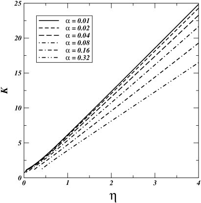
Figure 2: The $K$-factor versus $\eta$ for various values of $\alpha$.

We note that the center-of-mass energy $\sqrt{s}$ in units of the rest mass of the produced particle is a function of $\eta/\alpha$:

$${\sqrt{s}\over m}=\sqrt{2\left(1+{{\eta/\alpha}\over\sqrt{\eta^{2}/\alpha^{2}-1}}\right)}.$$ (42)

Various other kinematic variables, such as ${k/m}={\sqrt{s}/2m}$ and ${p/m}=\sqrt{{s/4m^{2}}-1}$ can be similarly expressed as a function of $\eta/\alpha$. From these relations and the relation between the $K$-factor and $\eta$ and $\alpha$, we can find out the $K$-factor for the production of a pair of particles in a specific kinematic configuration.

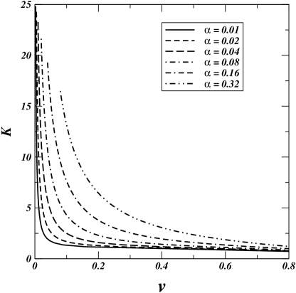
Figure 3: The $K$-factor versus the velocity $v$ for various values of $\alpha$.

We showed the behavior of the $K$-factor as a function of $\eta$ in Fig. 2 for various values of $\alpha$. The solid curve gives the $K$-factor for $\alpha=0.01$ and the dotted curve gives the $K$-factor for $\alpha=0.32$. For a fixed value of $\alpha$, the $K$-factor decreases as $\eta$ decreases. This is consistent with the expectation that the effects of the final-state interaction diminish as the velocity becomes relativistic. The limiting value is $K$=1 as $\eta\rightarrow\alpha$(or $v\rightarrow 1$). Figure 2 also shows that for a given value of $\eta$, the $K$-factor decreases as $\alpha$ increases. It should be noted that the same value of $\eta$ corresponds to different velocities $v$ for different values of $\alpha$. To see the effect of final-state interaction as a function of $\alpha$ for a fixed value of $v$, we plot in Fig. 3 the $K$-factor as a function of $v$. As one observes, when the velocity is fixed, the $K$-factor increases as the coupling constant increases, indicating a greater effect of the final-state interaction as $\alpha$ increases. For all values of $\alpha$, the $K$-factor decreases with $v$ and goes to unity as $v$ approaches 1. The decrease is very rapid for small values of $\alpha$.

Figure 4: The ratio between the $K$-factor and the Gamow factor for various values of $\alpha$.

It is of interest to see how the $K$-factor obtained here is different from the Gamow factor in non-relativistic physics. In Fig. 4$(b)$, we showed the ratio between the $K$-factor and the Gamow factor for various values of $\alpha$. As we expect, the ratio is almost 1 for weak coupling and the use of the Gamow factor is relatively safe there. However, if we increase $\alpha$ to 0.32, the ratio decreases significantly. The Gamow factor over-estimates the magnitude of the final-state interaction and therefore it cannot be used for the case with strong coupling. There is an effective screening of the long-range Coulomb interaction. As a consequence, the enhancement due to the long-range Coulomb-type interaction is reduced. It can also be observed in Fig. 4$b$ that the ratio of $K/G(\eta)$ is a relatively slowly varying function of $\eta$ for $\eta>1$ but drops down rapidly as $\eta$ decreases in the region of small $\eta$ (high $v$).

It is worth pointing out that the expansion of $\cal A$ in Eq. (35) is given as a series in powers of $p/\sqrt{\delta^{2}+k^{2}}$ which increases as the velocity $v$ increases. We still obtain convergent results for $v$ up to about 0.8, but there is a limit on using such an expansion for greater velocities where $p/\sqrt{\delta^{2}+k^{2}}$ is too large to allow for a convergent term-by-term summation. A different expansion method may be needed. Fortunately, the $K$-factor for this region is so close to unity that it can be taken to be unity without incurring much error.

We can compare the results we have obtained for the case of fermions with those for the previous case of bosons. We show in Fig.  4$a$ the ratio of $K/G(\eta)$ for the final state interaction of two bosons. The $K$ factor for bosons is slightly smaller than the $K$-factor for fermions and the difference is greater for larger values of $\alpha$. This means that the overestimations by the Gamow factor are larger in bosonic FSI/ISI than in fermionic one.

VI Conclusions and Discussions

When a pair of particles are subject to final-state interactions, the rate of their production is modified. There will be similar effects if the particles interact via initial-state interactions. The modification is simplest to be taken into account by using the $K$-factor. One calculates first the rate for the process when there were no initial- or final-state interactions, using, for example, the perturbation theory. The additional initial- or final-state interactions are then included by multiplying a $K$-factor as given by Eq. (8).

For Coulomb-type interactions, the $K$-factor has been traditionally taken to be the Gamow factor obtained as the absolute square of the wave function at the origin of the relative coordinate. With relativistic Coulomb wave functions, the wave function at the origin is infinite and the usual method is not applicable. The $K$-factor can be obtained as the overlap of the wave function with the Feynman amplitude.

Our investigation of the $K$-factor for the case of the production of a pair of scalar particles indicates that there are substantial deviations from the Gamow factor when the strength of the coupling is large. In particular, the proper treatment reduces the magnitude of the Gamow factor significantly. The reason for this reduction is that in the pair production, there is an effective screening of the Coulomb-type interaction arising from the effective “exchange” of one of the produced particles.

We have presented an explicit formula for the relativistic modification of the Gamow factor for the production of a pair of fermions. Numerical results are also obtained to show the magnitude of the $K$-factor. The results of the $K$-factor can be applied to a class of processes in which the fermion particles are produced and interacting with a Coulomb-type final-state interaction as for an example in the production of open charm pairs Tai04 ; Ada04 ; Adl04 . Such an application to the production of heavy quarks systems near the threshold will be of great interest.

References

- (1) H. A. Bethe and P. Morrison, Elementary Nuclear Theory, John Wiley and Sons, New York, 1956; J. M. Blatt and V. F. Weisskopf, Theoretical Nuclear Physics, John Wiley and Sons, New York, 1952, p. 731.
- (2) G. Gamow, Zeit. Phys. 51, 204 (1928), see also L. I. Schiff, Quantum Mechanics, McGraw-Hill Company, 1955, p. 142.
- (3) A. Sommerfeld, Atmobau und Spektralinien, Bd. 2. Braunschweig: Vieweg 1939
- (4) R. M. Barnett, M. Dine, and L. McLerran, Phys. Rev. D22, 594 (1980).
- (5) S. Güsken, J. H. Kühn, and P. M. Zerwas, Phys. Lett. 155B, 185 (1988).
- (6) V. Fadin and V. Khoze, Soviet Jour. Nucl. Phys. 48, 487 (1988).
- (7) V. Fadin, V. Khoze, and T. Sjöstrand, Zeit. Phys. C48, 613 (1990).
- (8) S. J. Brodsky, A. H. Hoang, J. H. Kühn, and T. Teubner, Phys. Lett. B359, 355 (1995).
- (9) L. Chatterjee and C. Y. Wong, Phys. Rev. C51, 2125 (1995).
- (10) C. Y. Wong and L. Chatterjee, Proceedings of Strangeness ’96 Meeting, Budapest, May 1996, ORNL-CTP-96-09 (hep-ph/9607316), published in Heavy Ion Phys. 4, 201 (1996).
- (11) C. Y. Wong and L. Chatterjee, Z. Phys. C75, 523 (1997).
- (12) J. H. Yoon and C. Y. Wong, Phys. Rev. C61, 044905 (2000).
- (13) J. H. Yoon and C. Y. Wong, J. Kor. Phys. Soc. 42, 423 (2003).
- (14) J. Schwinger, Particles, Sources, and Fields, (Addison-Wesley, New York, 1973), Vol.II, Chapters 4 and 5.
- (15) G. Baym and P. Braun-Munzinger, Nucl. Phys. A610 (1996) 286c-296c
- (16) M. E. Peskin and D. V. Schroeder, An Introduction to Quantum Field Theory, Addision Wesley Publishing Company, 1995.
- (17) H. W. Crater, Phys. Rev. A44, 7065 (1991).
- (18) I. T. Todorov, Phys. Rev. D3, 2351 (1971).
- (19) P. A. M. Dirac, Canad. J. Math. 2, 129 (1950); Proc. Roy. Soc. Sect. A 246, 326 (1958); Lectures on Quantum Mechanics (Yeshiva University, Hew York, 1964).
- (20) P. Van Alstine and H. W. Crater, J. Math. Phys. 23, 1997 (1982); H. W. Crater and P. Van Alstine, Ann. Phys. (N.Y.) 148, 57 (1983); H. W. Crater and P. Van Alstine, Phys. Rev. Lett. 53 , 1577 (1984).
- (21) P. Van Alstine and H. W. Crater, Phys. Rev. D34, 1932 (1986).
- (22) H. W. Crater and P. Van Alstine, Phys. Rev. D36, 3007 (1987).
- (23) H. W. Crater and P. Van Alstine, Phys. Rev. D37, 1982 (1988); H. W. Crater and P. Van Alstine, Found. Phys. 24, 297 (1994); H. W. Crater, R. Becker, Cheuk-Yin Wong, and P. Van Alstine, Phy. Rev. D46, 5117 (1992); H. W. Crater. Comp. Phys. 115 , 470 (1994); H. W. Crater and P. Van Alstine, J. Math. Phys. 31, 1998 (1990); H. Jallouli and H. Sazdjian, Phys. Lett. B366, 409 (1996); H. W. Crater, C. W. Wong, and C. Y. Wong, Intl. J. Mod. Phys.-E 5, 589 (1996); P. Long and H. W. Crater, J. Math. Phys. 39, 124 (1998).
- (24) A. Tai, J.Phys. G30, S809-S818 (2004).
- (25) J. Adams, , the STAR Collaboration, nucl-ex/0407006.
- (26) S. S. Adler , the PHENIX Collaboration, nucl-ex/0409028.