WM-04-123
JLAB-05-04-306
Some electromagnetic properties of the nucleon from
Relativistic Chiral Effective Field Theory

Abstract

Considering the magnetic moment and polarizabilities of the nucleon we emphasize the need for relativistic chiral EFT calculations. Our relativistic calculations are done via the forward-Compton-scattering sum rules, thus ensuring the correct analytic properties. The results obtained in this way are equivalent to the usual loop calculations, provided no heavy-baryon expansion or any other manipulations which lead to a different analytic structure (e.g., infrared regularization) are made. The Baldin sum rule can directly be applied to calculate the sum of nucleon polarizabilities. In contrast, the GDH sum rule is practically unsuitable for calculating the magnetic moments. The breakthrough is achieved by taking the derivatives of the sum rule with respect to the anomalous magnetic moment. As an example, we apply the derivative of the GDH sum rule to the calculation of the magnetic moment in QED and reproduce the famous Schwinger’s correction from a tree-level cross-section calculation. As far as the nucleon properties are concerned, we focus on two issues: 1) chiral behavior of the nucleon magnetic moment and 2) reconciliation of the chiral loop and $\Delta$-resonance contributions to the nucleon magnetic polarizability.

1 GDH sum rule and its derivatives

Consider the elastic scattering of a photon on a target with spin $s$ (real Compton scattering). The forward-scattering amplitude of this process is characterized by $2s+1$ scalar functions which depend on a single kinematic variable, e.g., the photon energy $\omega$. In the low-energy limit each of these functions corresponds to an electromagnetic moment — charge, magnetic dipole, electric quadrupole, etc. — of the target. For example in the case of the nucleon, the forward Compton amplitude is generally written as

$$T(\omega)=\vec{\varepsilon}^{\prime}\cdot\vec{\varepsilon}\,f(\omega)+i\,\vec{\sigma}\cdot(\vec{\varepsilon}^{\prime}\times\vec{\varepsilon})\,g(\omega)\,,$$ (1)

where $\vec{\varepsilon}$, $\vec{\varepsilon}^{\prime}$ is the polarization vector of the incident and scattered photon, respectively; $\vec{\sigma}$ are the Pauli matrices representing the dependence on the nucleon spin. The two scalar functions have the following low-energy expansion,

$$f(\omega) = -\frac{e^{2}}{4\pi M}+(\alpha_{E}+\beta_{M})\,\omega^{2}+{\mathcal{O}}(\omega^{4})\ ,$$ (2a)

$$g(\omega) = -\frac{e^{2}\kappa^{2}}{8\pi M^{2}}\,\omega+\gamma_{0}\omega^{3}+{\mathcal{O}}(\omega^{5})\ ,$$ (2b)

hence in the low-energy limit they are given in terms of the nucleon charge $e$ and the anomalous magnetic moment (a.m.m.) $\kappa$. The next-to-leading order terms are specified by the nucleon electric ($\alpha_{E}$), magnetic ($\beta_{M}$), and forward spin ($\gamma_{0}$) polarizabilities.

To derive the sum rules (SRs) for these quantities one assumes the scattering amplitude is an analytic function of $\omega$ everywhere but the real axis. This allows us to write the real parts of functions $f(\omega)$ and $g(\omega)$ as a dispersion integral of their imaginary parts. The latter, on the other hand, can be related to the total photoabsorption cross-sections by using the optical theorem,

$$\mbox{Im}\ f(\omega) = \frac{\omega}{8\pi}\left[\sigma_{1/2}(\omega)+\sigma_{3/2}(\omega)\right]\,,$$ (3a)

$$\mbox{Im}\ g(\omega) = \frac{\omega}{8\pi}\left[\sigma_{1/2}(\omega)-\sigma_{3/2}(\omega)\right]\,,$$ (3b)

where $\sigma_{\lambda}$ is the double-polarized total cross-section of the photoabsorption processes. Averaging over the polarization of initial particles gives the total unpolarized cross-section, $\sigma_{T}=\mbox{\small{$\frac{1}{2}$}}(\sigma_{1/2}+\sigma_{3/2})$.

Finally one uses the crossing symmetry, meaning that the Compton amplitude of Eq. (1) must be invariant under $\varepsilon^{\prime}\leftrightarrow\varepsilon$, $\omega\rightarrow-\omega$, and hence $f$ is an even and $g$ an odd function of energy:$f(\omega)=f(-\omega)$, $g(\omega)=-g(-\omega)$.

Going through these steps one arrives at the following result (see, e.g., [1] for more details):

$$f(\omega) = \frac{1}{2\pi^{2}}\,\int_{0}^{\infty}\frac{\sigma_{T}(\omega^{\prime})}{\omega^{\prime 2}-\omega^{2}-i\epsilon}\,\omega^{\prime 2}\,d\omega^{\prime}\ .$$ (4)

$$g(\omega) = -\frac{\omega}{4\pi^{2}}\,\int_{0}^{\infty}\frac{\Delta\sigma(\omega^{\prime})}{\omega^{\prime 2}-\omega^{2}-i\epsilon}\,\omega^{\prime}\,d\omega^{\prime}\ ,$$ (5)

with $\Delta\sigma\equiv\sigma_{3/2}-\sigma_{1/2}$. These relations can be expanded in energy to obtain the SRs for the different static properties introduced in Eq. (2). In this way we can obtain the Baldin SR:

$$\alpha_{E}+\beta_{M}=\frac{1}{2\pi^{2}}\,\int_{0}^{\infty}\,\frac{\sigma_{T}(\omega^{\prime})}{\omega^{\prime 2}}\,d\omega^{\prime}\ ,$$ (6)

the Gerasimov-Drell-Hearn (GDH) SR:

$$\frac{e^{2}\kappa^{2}}{2M^{2}}=\frac{1}{\pi}\int_{0}^{\infty}\,\frac{\Delta\sigma(\omega)}{\omega}\,d\omega\,,$$ (7)

and a SR for the forward spin polarizability:

$$\gamma_{0}=\,-\,\frac{1}{4\pi^{2}}\,\int_{0}^{\infty}\,\frac{\Delta\sigma(\omega)}{\omega^{3}}\,d\omega\ .$$ (8)

As we all now know, impressive experimental programs to measure the total photoabsorption cross-sections of the nucleon have recently been carried out at ELSA and MAMI (for a review see Ref. [2]). These measurements are needed for an empirical test of the GDH SR, as well as for phenomenological estimates of $\alpha_{E}+\beta_{M}$ and $\gamma_{0}$ via the other two SRs. The GDH SR is particularly interesting because both the left- and right-hand-side of this SR can reliably be measured, thus providing a test of the fundamental principles (such as unitarity and analyticity) which go into its derivation.

Testing theories by using these SRs could also be fun and even useful in instances when the consistency of the theory is not transparent. Let us, for example, have a look at the left- and right-hand-sides of the GDH SR for the electron in QED. To lowest order in the fine-structure constant, $\alpha=e^{2}/4\pi$, the photoabsorption cross-section is given by the tree-level Compton scattering cross-section [3]:

$$\Delta\sigma(\omega)=\frac{2\pi\alpha^{2}}{M\omega}\left[2+{2\omega^{2}\over(M+2\omega)^{2}}-\left(1+{M\over\omega}\right)\,\ln\left(1+\frac{2\omega}{M}\right)\right]+O(\alpha^{3}).$$ (9)

On the other hand, the one-loop contribution to the electron a.m.m. is of order $\alpha$ and therefore the lhs has no contribution of $\alpha^{2}$. Fortunately, the GDH integral over the tree-level cross-section Eq. (9) vanishes, and thus, at this order, everything works out:

$$0=0$$ (10)

as one could expect for such a fortunate theory as QED. At order $\alpha^{3}$ the lhs receives the contribution in the form of Schwinger’s correction: $\kappa=\alpha/2\pi$. The calculation of cross sections at this order is quite a formidable task as it requires the knowledge of Compton scattering amplitude to one-loop, inclusion of the pair-production channel, and so on, cf. [4]. Instead, I want to follow a much simpler way to do calculations at this level [5].

Let us introduce a ‘classical’ (or ’trial’) value of the a.m.m., $\kappa_{0}$. At the level of the Lagrangian this amounts to introducing a Pauli term for our spin-1/2 field:

$${\cal L}_{\mbox{\small Pauli}}=(i\kappa_{0}/4M)\,\bar{\psi}\,\sigma_{\mu\nu}\,\psi\,F^{\mu\nu}\,,$$ (11)

where $F$ is the electromagnetic field tensor and $\sigma_{\mu\nu}=(i/2)[\gamma_{\mu},\gamma_{\nu}]$. In the end we can put $\kappa_{0}$ equal to zero, but for now the total value of the a.m.m. is $\kappa=\kappa_{0}+\delta\kappa$, with $\delta\kappa$ being the quantum effects. Note that $\delta\kappa$ and the total cross-sections become explicitly dependent on $\kappa_{0}$. To get something new out of this we need to start taking derivatives of the GDH SR with respect to $\kappa_{0}$:

$$(4\pi^{2}\alpha/M^{2})\,\kappa\,\kappa^{\prime} = \int_{0}^{\infty}\!\Delta\sigma^{\prime}(\omega)\,\frac{d\omega}{\omega}\,,$$ (12)

$$(4\pi^{2}\alpha/M^{2})\,(\kappa^{\prime 2}+\kappa\,\kappa^{\prime\prime}) = \int_{0}^{\infty}\!\Delta\sigma^{\prime\prime}(\omega)\,\frac{d\omega}{\omega}\,,$$ (13)

and so on. Now observe that to lowest order in $\alpha$ these relations simply read as

$$(4\pi^{2}\alpha/M^{2})\,n\,\kappa^{(n-1)}=\int_{0}^{\infty}\!\!\Delta\sigma^{(n)}(\omega)\,\frac{d\omega}{\omega}\,$$ (14)

where $n$ is the order of the derivative with respect to $\kappa_{0}$. This allows us in principle to compute $\kappa$ to order $\alpha^{k}$ by using $k$th, $(k-1)$th, etc., derivatives of the cross-section computed, respectively, to order $\alpha^{k+1}$, $\alpha^{k}$, etc. In this way, to lowest order we have the following sum rule:

$$(4\pi^{2}\alpha/M^{2})\,\kappa=\int_{0}^{\infty}\!\left.\Delta\sigma^{\prime}(\omega)\right|_{\kappa_{0}=0}\,\frac{d\omega}{\omega}\,.$$ (15)

The striking feature of this sum rule is the linear relation between the a.m.m. and the photoabsorption cross section, in contrast to the GDH SR where the relation is quadratic. This restores the “balance of difficulty” in the two methods of calculating this quantity: the sum rule or the usual loop technique.

Although the cross-section quantity $\Delta\sigma^{\prime}$ is not an observable, it is very clear how to determine it within a given theory. The first derivative of the tree-level cross-section with respect to $\kappa_{0}$, at $\kappa_{0}=0$, in QED takes the form [5]:

$$\left.\Delta\sigma^{\prime}(\omega)\right|_{\kappa_{0}=0}=\frac{2\pi\alpha^{2}}{M\omega}\left[6-{2M\omega\over(M+2\omega)^{2}}-\left(2+{3M\over\omega}\right)\,\ln\left(1+\frac{2\omega}{M}\right)\right].$$ (16)

It is then not difficult to find that

$$\frac{1}{\pi}\int\limits_{0}^{\infty}\!\left.\Delta\sigma^{\prime}(\omega)\right|_{\kappa_{0}=0}\,{d\omega\over\omega}=\frac{2\alpha^{2}}{M^{2}}\,.$$ (17)

Substituting this result in the linearized SR, Eq. (15), we obtain $\kappa=\alpha/2\pi$. Thus, the Schwinger’s one-loop result is reproduced here by computing only a (derivative of the) tree-level Compton scattering cross-section and then performing a GDH integral.

2 Magnetic moments and their chiral extrapolation

Consider now the theory of nucleons interacting with pions via pseudovector coupling:

$${\cal L}_{\pi NN}=\frac{g}{2M}\,\bar{\psi}\,\gamma^{\mu}\,\gamma^{5}\,\tau^{a}\,\psi\,\partial_{\mu}\pi^{a},$$ (18)

where $g$ is the pion-nucleon coupling constant, $\tau^{a}$ are isospin Pauli matrices, $\pi^{a}$ is the isovector pion field. For our purposes this Lagrangian is sufficient to obtain the leading order results of chiral perturbation theory.

Figure 1: Tree-level pion photoproduction graphs. The circled vertex corresponds to the Pauli coupling.

To lowest order in $g$ the photoabsorption cross section in this theory is dominated by the single pion photoproduction graphs as displayed in Fig. 1. We find for the corresponding GDH cross sections:

$$\Delta\sigma^{(\pi^{0}p)} = \frac{\pi C}{M^{2}x^{2}}\,\left[(2\alpha\bar{s}+1-x)\ln\frac{\alpha+\lambda}{\alpha-\lambda}-2\lambda[x(\alpha-2)+\bar{s}(\alpha+2)]\right],\qquad$$ (19a)

$$\Delta\sigma^{(\pi^{+}n)} = \frac{2\pi C}{M^{2}x^{2}}\,\left[-\mu^{2}\ln\frac{\beta+\lambda}{\beta-\lambda}+2\lambda(\bar{s}\beta-x\alpha)\right],$$ (19b)

$$\Delta\sigma^{(\pi^{0}n)} = 0,$$ (19c)

$$\Delta\sigma^{(\pi^{-}p)} = \frac{2\pi C}{M^{2}x^{2}}\,\left[-\mu^{2}\ln\frac{\beta+\lambda}{\beta-\lambda}+(2\alpha\bar{s}-1-x)\ln\frac{\alpha+\lambda}{\alpha-\lambda}-2\bar{s}\lambda\right],$$ (19d)

where $C=\left(eg/4\pi\right)^{2}$, $\mu=m_{\pi}/M$, $m_{\pi}$ is the pion mass, and

$$s=M^{2}+2M\omega,\,\,\,\bar{s}=s/M^{2},$$ (20a)

$$\alpha=(s+M^{2}-m_{\pi}^{2})/2s,$$ (20b)

$$\beta=(s-M^{2}+m_{\pi}^{2})/2s=1-\alpha,$$ (20c)

$$\lambda=(1/2s)\sqrt{s-(M+m_{\pi})^{2}}\sqrt{s-(M-m_{\pi})^{2}}\,.$$ (20d)

As in the case of QED, the anomalous magnetic moment corrections start at ${\cal O}(g^{2})$, implying that the $lhs$ of the GDH SR begins at ${\cal O}(g^{4})$. Since the tree-level cross sections are ${\cal O}(g^{2})$, we must require that

$$\int\limits_{\omega_{\rm th}}^{\infty}{d\omega\over\omega}\,\Delta\sigma^{(I)}(\omega)=0,\,\,\,\,\mbox{for $I=\pi^{0}p,\,\pi^{+}n,\,\pi^{0}n,\pi^{-}p$},$$ (21)

where $\omega_{\rm th}=m_{\pi}(1+m_{\pi}/2M)$ is the threshold of the pion photoproduction reaction. This requirement is indeed verified for the expressions given in Eq. (19) —the consistency of GDH SR is maintained in this theory for each of the pion production channels.

We now turn our attention to the linearized GDH sum rule. In this case we first introduce Pauli moments $\kappa_{0p}$ and $\kappa_{0n}$ for the proton and the neutron, respectively. The dependence of the cross-sections on these quantities can generally be presented as:

$$\Delta\sigma(\omega;\,\kappa_{0p},\,\kappa_{0n}) = \Delta\sigma(\omega)+\kappa_{0p}\,\Delta\sigma_{1p}(\omega)+\kappa_{0n}\,\Delta\sigma_{1n}(\omega)$$ (22)

$$+ \kappa_{0p}^{2}\,\Delta\sigma_{2p}(\omega)+\kappa_{0n}^{2}\,\Delta\sigma_{2n}(\omega)+\kappa_{0p}\,\kappa_{0n}\,\Delta\sigma_{1p1n}(\omega)+\ldots.$$

Furthermore, we introduce proton and neutron photoproduction cross sections $\Delta\sigma^{(p)}$ and $\Delta\sigma^{(n)}$ and express the corresponding GDH SRs and their first derivatives. Analogous to the QED case, we obtain :

• the GDH SRs:

  $$\frac{2\pi\alpha}{M^{2}}\,\kappa_{p}^{2}=\frac{1}{\pi}\int\limits_{\omega_{th}}^{\infty}\!\frac{d\omega}{\omega}\,\Delta\sigma^{(p)},\,\,\,\,\frac{2\pi\alpha}{M^{2}}\,\kappa_{n}^{2}=\frac{1}{\pi}\int\limits_{\omega_{th}}^{\infty}\!\frac{d\omega}{\omega}\,\Delta\sigma^{(n)},$$ (23a)

• the linearized SRs (valid to leading order in the coupling $g$):

  $$\frac{4\pi\alpha}{M^{2}}\,\kappa_{p}=\frac{1}{\pi}\int\limits_{\omega_{th}}^{\infty}\!\frac{d\omega}{\omega}\,\Delta\sigma_{1p}^{(p)},\,\,\,\,\frac{4\pi\alpha}{M^{2}}\,\kappa_{n}=\frac{1}{\pi}\int\limits_{\omega_{th}}^{\infty}\!\frac{d\omega}{\omega}\,\Delta\sigma_{1n}^{(n)},$$ (23b)

• the consistency conditions (valid to leading order in the coupling $g$):

  $$0=\frac{1}{\pi}\int\limits_{\omega_{th}}^{\infty}\!\frac{d\omega}{\omega}\,\Delta\sigma_{1n}^{(p)},\,\,\,\,0=\frac{1}{\pi}\int\limits_{\omega_{th}}^{\infty}\!\frac{d\omega}{\omega}\,\Delta\sigma_{1p}^{(n)}.$$ (23c)

The first derivatives of the cross-sections that enter in Eq. (23), to leading order in $g$, arise through the interference of Born graphs Fig. 1(a) with the graphs in Fig. 1(b) and we find:

$$\Delta\sigma_{1p}^{(p)}\equiv\Delta\sigma_{1p}^{(\pi^{0}p)}+\Delta\sigma_{1p}^{(\pi^{+}n)} = \frac{\pi C}{M^{2}x^{2}}\left\{2x\lambda[4+(1-2\alpha)(2+\bar{s}+2x)]+2\bar{s}\lambda(\alpha+2)\right.$$ (24a)

$$- \left.\mu^{2}x\ln\frac{\beta+\lambda}{\beta-\lambda}+(2\alpha\bar{s}+1-x)\ln\frac{\alpha+\lambda}{\alpha-\lambda}\right\},$$

$$\Delta\sigma_{1n}^{(n)}\equiv\Delta\sigma_{1n}^{(\pi^{0}n)}+\Delta\sigma_{1n}^{(\pi^{-}p)} = \frac{\pi C}{M^{2}x}\left\{2\lambda(2+2x-\bar{s})+\mu^{2}\ln\frac{\beta+\lambda}{\beta-\lambda}-\ln\frac{\alpha+\lambda}{\alpha-\lambda}\right\},\qquad$$ (24b)

$$\Delta\sigma_{1n}^{(p)}\equiv\Delta\sigma_{1n}^{(\pi^{0}p)}+\Delta\sigma_{1n}^{(\pi^{+}n)} = \frac{2\pi C}{M^{2}x^{2}}\left\{\ln\frac{\alpha+\lambda}{\alpha-\lambda}+2\lambda(x\beta-\bar{s}\alpha)\right\},$$ (24c)

$$\Delta\sigma_{1p}^{(n)}\equiv\Delta\sigma_{1p}^{(\pi^{0}n)}+\Delta\sigma_{1p}^{(\pi^{-}p)} = \frac{2\pi C}{M^{2}x^{2}}\left\{(2\bar{s}\alpha-x)\,\ln\frac{\alpha+\lambda}{\alpha-\lambda}+2\lambda(x-2\bar{s})\right\}.$$ (24d)

Using the latter two expressions we easily verify the consistency conditions given in Eq. (23c), while, employing the linearized SRs, we obtain:

$$\kappa_{p}^{\rm(loop)} = \frac{M^{2}}{\pi e^{2}}\int\limits_{\omega_{\mathrm{th}}}^{\infty}\!\frac{d\omega}{\omega}\Delta\sigma_{1p}^{(p)}$$ (25a)

$$= \frac{g^{2}}{(4\pi)^{2}}\left\{1-\frac{\mu\,\left(4-11{\mu}^{2}+3{\mu}^{4}\right)}{\sqrt{1-\mbox{\small{$\frac{1}{4}$}}{\mu}^{2}}}\arccos\frac{\mu}{2}-6{\mu}^{2}+2{\mu}^{2}\left(-5+3\,{\mu}^{2}\right)\ln\mu\right\},$$

$$\kappa_{n}^{\rm(loop)} = \frac{M^{2}}{\pi e^{2}}\int\limits_{\omega_{\mathrm{th}}}^{\infty}\!\frac{d\omega}{\omega}\Delta\sigma_{1n}^{(n)}=\frac{-2g^{2}}{(4\pi)^{2}}\left\{2-\frac{\mu\,(2-\mu^{2})}{\sqrt{1-\mbox{\small{$\frac{1}{4}$}}{\mu}^{2}}}\arccos\frac{\mu}{2}-2\mu^{2}\ln\mu\right\}.$$ (25b)

We have checked that Eq. (25) agrees with the one-loop calculation done by using the standard Feynman-parameter technique. It is interesting that, to this order, the pseudoscalar pion-nucleon coupling gives exactly the same result.

On the other hand, this result does not agree with the covariant ChPT calculation of Ref. [6], which are based upon the “infrared-regularization” procedure of Becher and Leutwyler. The discrepancy is apparently due to the fact that the ”infrared-regularized” loop amplitudes do not satisfy the usual dispersion relations. Their analytic properties in the energy plane are complicated by an additional cut due to explicit dependence on $\sqrt{s}$. In other words, they do not obey the analyticity constraint which is imposed on the sum rule calculation.

It is instructive to examine the chiral behavior of the one-loop result for the nucleon magnetic moment. Expanding Eq. (25) around the chiral limit ($m_{\pi}=0$), which incidentally corresponds here with the heavy-baryon expansion, we have

$$\kappa_{p}^{\rm(loop)} = \frac{g^{2}}{(4\pi)^{2}}\left\{1-2\pi\mu-2\,(2+5\ln\mu)\,\mu^{2}+\frac{21\pi}{4}\,\mu^{3}+O(\mu^{4})\right\},$$ (26)

$$\kappa_{n}^{\rm(loop)} = \frac{g^{2}}{(4\pi)^{2}}\left\{-4+2\pi\mu-2\,(1-2\ln\mu)\,\mu^{2}-\frac{3\pi}{4}\,\mu^{3}+O(\mu^{4})\right\}.$$ (27)

The term linear in pion mass (recall that $\mu=m_{\pi}/M$) is the well-known leading nonanalytic (LNA) correction. On the other hand, expanding the same expressions around the large $m_{\pi}$ limit we find

$$\kappa_{p}^{\rm(loop)} = \frac{g^{2}}{(4\pi)^{2}}\,(5-4\ln\mu)\frac{1}{\mu^{2}}+O(\mu^{-4}),$$ (28)

$$\kappa_{n}^{\rm(loop)} = \frac{g^{2}}{(4\pi)^{2}}\,2(3-4\ln\mu)\frac{1}{\mu^{2}}+O(\mu^{-4}).$$ (29)

What is intriguing here is that the one-loop correction to the nucleon a.m.m. for heavy quarks behaves as $1/m_{quark}$ (where $m_{quark}\sim m_{\pi}^{2})$, precisely as expected from a constituent quark-model picture. Here this is a result of subtle cancellations in Eq. (25) taking place for large values of $m_{\pi}$. In contrast, the infrared regularization procedure [6] gives the result which exhibits pathological behavior with increasing pion mass and diverges for $m_{\pi}=2M$.

Since the expressions in Eq. (25) have the correct large $m_{\pi}$ behavior they should be better suited for the chiral extrapolations of the lattice results than the usual heavy-baryon expansions or the “infrared-regularized” relativistic theory. This point is clearly demonstrated by Fig. 2, where we plot the $m_{\pi}$-dependence of the full [Eq. (25)], heavy-baryon, and infrared-regularization [6] leading order result for the magnetic moment of the proton and the neutron, in comparison to recent lattice data [7]. In presenting these results we have added a constant shift (counter-term $\kappa_{0}$) to the magnetic moment, i.e.,

$$\mu_{p} = (1+\kappa_{0p}+\kappa_{p}^{\rm(loop)})(e/2M),$$ (30)

$$\mu_{n} = (\kappa_{0n}+\kappa_{n}^{\rm(loop)})(e/2M)$$ (31)

and fitted it to the known experimental value of the magnetic moment at the physical pion mass, $\mu_{p}\simeq 2.793$ and $\mu_{n}\simeq-1.913$, shown by the open diamonds in the figure. For the value of the $\pi NN$ coupling constant we have used $g^{2}/4\pi=13.5$. The $m_{\pi}$-dependence away off the physical point is then a prediction of the theory. The figure clearly shows that the SR results, shown by the dotted lines, is in a better agreement with the behavior obtained in lattice gauge simulations.

It is therefore tempting to use the SR results for the parametrization of lattice data. For example, we consider the following two-parameter form:

$$\mu_{p} = \left(1+\frac{\tilde{\kappa}_{0p}}{1+a_{p}m_{\pi}^{2}}+\kappa_{p}^{\rm(loop)}\right)\frac{e}{2M},$$ (32a)

$$\mu_{n} = \left(\frac{\tilde{\kappa}_{0n}}{1+a_{n}m_{\pi}^{2}}+\kappa_{n}^{\rm(loop)}\right)\frac{e}{2M}\,,$$ (32b)

where $\tilde{\kappa}_{0p}$ and $\tilde{\kappa}_{0n}$ are fixed to reproduce the experimental magnetic moments at the physical $m_{\pi}$. The parameter $a$ can be fitted to lattice data. The solid curves in Fig. 2 represent the result of such a single parameter fit to the lattice data of Ref. [7] for the proton and neutron respectively, where $a_{p}=1.6/M^{2}$ and $a_{n}=1.05/M^{2}$, $M$ is the physical nucleon mass.

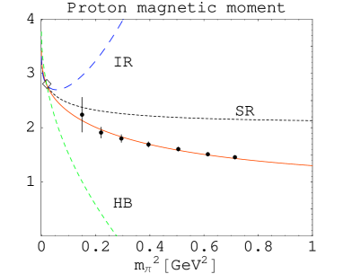
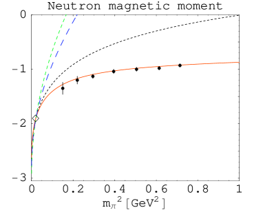
Figure 2: Chiral behavior of proton and neutron magnetic moments (in nucleon magnetons) to one loop compared with lattice data. “SR” (dotted lines): our one-loop relativistic result, “IR” (blue long-dashed lines): infrared-regularized relativistic result, “HB” (green dashed lines): LNA term in the heavy-baryon expansion. Red solid lines: single-parameter fit based on our SR result. Data points are results of lattice simulations. The open diamonds represent the experimental values at the physical pion mass.

3 The nucleon polarizability puzzle

It is well-known that the Heavy-Baryon ChPT (HBChPT) at order $p^{3}$ gives a remarkable prediction for the electric and magnetic polarizabilities of the nucleon:

$$\alpha_{E}^{(HBLO)}=\frac{5\pi\alpha}{6\,m_{\pi}}\left(\frac{g_{A}}{4\pi f_{\pi}}\right)^{2}=12.2\times 10^{-4}~{}\mbox{fm}^{3},$$ (33a)

$$\beta_{M}^{(HBLO)}=\frac{\pi\alpha}{12\,m_{\pi}}\left(\frac{g_{A}}{4\pi f_{\pi}}\right)^{2}=1.2\times 10^{-4}~{}\mbox{fm}^{3}\,,$$ (33b)

where $g_{A}\simeq 1.26$, $f_{\pi}\simeq 93$ MeV (related to the $\pi NN$ coupling constant used in the previous section via the Goldberger-Triemann relation: $g_{A}/f_{\pi}=g/M$). Remarkable, because this is a true prediction of HBChPT (there are no counter-terms at this order) and because it appears to be in a very good agreement with experiment.

For now, I am concerned only with the sum of these polarizabilities. On the experimental side, a recent determination from the Baldin’s sum gives [8]:

$$(\alpha_{E}+\beta_{M})_{p} = (13.69\pm 0.14)\times 10^{-4}~{}{\rm{fm}}^{3}\ ,$$

$$(\alpha_{E}+\beta_{M})_{n} = (14.40\pm 0.66)\times 10^{-4}~{}{\rm{fm}}^{3}\ ,$$ (34)

for proton and neutron, respectively.

It is also well-known that the $\Delta(1232)$-resonance excitation gives a large effect to the magnetic polarizability. To quantify this effect we use the following Lagrangian for the $\gamma N\Delta$ coupling [9, 10]:

$${\mathcal{L}}_{\gamma N\Delta}=\frac{3\,e}{2M(M+M_{\Delta})}\,\overline{\Psi}\,T_{3}^{\dagger}\left(ig_{M}\tilde{F}^{\mu\nu}-g_{E}\gamma_{5}F^{\mu\nu}\right)\,\partial_{\mu}\psi_{\nu}+\mbox{H.c.},$$ (35)

where $\Psi$ is the nucleon field, $\psi_{\mu}$ is the isospin-3/2 spin-3/2 vector-spinor field of the $\Delta$-isobar, $T_{3}$ is the isospin $N\Delta$ transition matrix. The coupling constants can be deduced from the empirical knowledge of the $\gamma N\rightarrow\Delta$ transition strength. Based on the Particle Data Group values for M1 and E2 we estimate $g_{M}\simeq 3$ and $g_{E}\simeq-1$.

Figure 3: The $\Delta$-excitation graphs.

Computing the sum of the $s$- and $u$-channel $\Delta$ contributions, Fig. 3, to the polarizabilities one finds (see [10] for more details):

$$\alpha_{E}^{(\Delta)} = -\frac{2\alpha\,g_{E}^{2}}{(M+M_{\Delta})^{3}}=-0.1\times 10^{-4}~{}\mbox{fm}^{3}$$ (36a)

$$\beta_{M}^{(\Delta)} = \frac{2\alpha g_{M}^{2}}{(M+M_{\Delta})^{2}}\frac{1}{M_{\Delta}-M}=7.3\times 10^{-4}~{}\mbox{fm}^{3}.$$ (36b)

So, while the HBChPT without Delta’s is in a good agreement with experiment, HBChPT with Delta’s is not at all. Puzzling… One would expect that including the $\Delta$ would improve the situation, extend the limit of applicability of our theory higher in energy, into the resonance region.

There are suggestions voiced now and then that the effect of the $\Delta$ is canceled by the $\sigma$-meson exchange, or correlated two-pion exchange. In EFT language this corresponds to canceling the $\Delta$ contribution by an effect which formally is of higher order in power counting than the $\Delta$ contribution. This kind of scenario has recently been explored in Ref. [11] where counter-terms of $O(p^{4})$ were “promoted” to lower order in order to cancel $\beta_{M}^{(\Delta)}$ .

Here I would like to argue that possibly there is a more natural explanation within the relativistic chiral EFT. To find the leading order prediction of chiral loops relativistically we have computed the unpolarized total cross-sections, corresponding to the Born graphs of single-pion photoproduction [12]:

$$\sigma^{(\pi^{0}p)} = \frac{\pi C}{M\omega^{3}}\,\left\{[\omega^{2}-\mu^{2}\alpha\,s]\,\ln\frac{\alpha+\lambda}{\alpha-\lambda}+2\lambda\left[\omega^{2}(\alpha-2)1+s\mu^{2}\right]\right\}$$

$$\sigma^{(\pi^{+}n)} = \frac{2\pi C}{M\omega^{3}}\,\left[-\beta\,s\,\mu^{2}\ln\frac{\beta+\lambda}{\beta-\lambda}+2\lambda\,(\alpha\,\omega^{2}+s\,\mu^{2})\right],$$ (37a)

$$\sigma^{(\pi^{0}n)} = 0,$$

$$\sigma^{(\pi^{-}p)} = \frac{2\pi C}{M\omega^{3}}\,\left\{\omega^{2}\ln\frac{\alpha+\lambda}{\alpha-\lambda}-\mu^{2}(s\beta-\mu^{2}M^{2})\,\ln\frac{\beta+\lambda}{\beta-\lambda}\,\frac{\alpha+\lambda}{\alpha-\lambda}+2s\mu^{2}\lambda\right\}.$$ (37b)

Substituting these expressions into the Baldin SR, Eq. (6), we obtain:

$$(\alpha_{E}+\beta_{M})_{p}^{(RLO)} = \frac{e^{2}g^{2}}{16\pi^{3}M^{3}}\left\{[3(1-4\mu^{2}+2\mu^{4})+\mbox{$\frac{1}{3}$}\mu^{2}]\ln\mu+\frac{406-737\mu^{2}+304\mu^{4}-36\mu^{6}}{6(4-\mu^{2})^{2}}\right.$$ (38a)

$$+ \left.\frac{44-788\mu^{2}+1500\mu^{4}-899\mu^{6}+215\mu^{8}-18\mu^{10}}{3\mu(4-\mu^{2})^{5/2}}\,{\rm arctg}{\sqrt{\frac{4}{\mu^{2}}-1}}\,\right\}\,,$$

$$(\alpha_{E}+\beta_{M})_{n}^{(RLO)} = \!\frac{e^{2}g^{2}}{16\pi^{3}M^{3}}\left\{\ln\mu+\frac{1}{(4-\mu^{2})^{2}}\left[\frac{2(2-3\mu^{2})(11-5\mu^{2})-3\mu^{6}}{3\mu\sqrt{4-\mu^{2}}}\,{\rm arctg}{\sqrt{\frac{4}{\mu^{2}}-1}}+5-\mu^{2}\right]\right\}.$$

Note that the same result is obtained in the conventional one-loop calculation [13]. The semi-relativistic (or, in this case also, chiral) expansion goes as follows:

$$(\alpha_{E}+\beta_{M})_{p}^{(RLO)} = \frac{e^{2}g^{2}}{(4\pi)^{2}M^{3}}\frac{11}{48\mu}\left(1+\frac{48(4+3\ln\mu)}{11\pi}\mu-\frac{1521}{88}\mu^{2}+\ldots\right)$$ (39a)

$$(\alpha_{E}+\beta_{M})_{n}^{(RLO)} = \frac{e^{2}g^{2}}{(4\pi)^{2}M^{3}}\frac{11}{48\mu}\left(1+\frac{4(1+12\ln\mu)}{11\pi}\mu-\frac{117}{88}\mu^{2}+\ldots\right)$$ (39b)

or, numerically (using $$g^{2}/4\pi=13.8 M=0.9383 \mu=0.148$$, GeV, ),

$$(\alpha_{E}+\beta_{M})_{p}^{(RLO)} = 14.5-5.2-5.5+\ldots=5.3$$ (39c)

$$(\alpha_{E}+\beta_{M})_{n}^{(RLO)} = 14.5-5.5-0.4+\ldots=8.7$$ (39d)

in the usual units. (The total values are consistent with L’vov’s numerical calculation [14], if we use $g^{2}/4\pi=14.2$. From that calculation it is clear that a lot of the reduction in the value of the sum affects the magnetic polarizability.)

Therefore, as one can see, the fully relativistic leading order result is substantially different from the non-relativistic (heavy-baryon) limit. The relativistic corrections which are suppressed by $m_{\pi}/M\simeq 1/7$, and hence are supposed to be small, appear with large coefficients and actually are not that small. The good news is that this apparently allows us to accommodate the large effect of the $\Delta$ isobar. In fact, the $\Delta$ contribution now improves the agreement with experiment. Adding the RLO and $\Delta$ numbers we have:

$$(\alpha_{E}+\beta_{M})_{p}^{(RLO+\Delta)} = 5.3+7.2=12.5\times 10^{-4}~{}{\rm{fm}}^{3}$$ (40)

$$(\alpha_{E}+\beta_{M})_{n}^{(RLO+\Delta)} = 8.7+7.2=15.9\times 10^{-4}~{}{\rm{fm}}^{3}.$$ (41)

At this order there is also an effect of $\pi\Delta$ chiral loops, but those are not yet computed relativistically.

4 Conclusion

The chiral EFT of QCD provides a description of the low-energy hadronic reactions and that allows one to extract hadron properties from experiments. On the other hand, it predicts the chiral behavior of these properties and that allows one to make a link to the lattice QCD calculations. These are the two fronts which at present make the chiral EFT indispensable in relating QCD to low-energy observables. The purpose of this talk is to demonstrate, on simple examples of nucleon magnetic moment and polarizabilities, that manifestly relativistic calculations do a better job than the “heavy-baryon” ones on both fronts.

The calculations done in this work were based on the real-Compton-scattering sum rules, such as GDH and Baldin sum rules. However, the results are not different from what one would obtained in the usual loop calculations, provided no manipulations (e.g., infrared regularization) which change the analytic structure are made. As is shown in the works of Gegelia et al. [15], there is no problem with power-counting in this, straightforward, formulation of covariant ChPT, if the renormalization scale is set in a suitable way.

References

[1]
D. Drechsel, B. Pasquini and M. Vanderhaeghen,
Phys. Rept. 378 (2003) 99.
[2]
D. Drechsel and L. Tiator,
arXiv:nucl-th/0406059;
see also contributions of R. Beck and P. Grabmayr in these proceedings.
[3] G. Altarelli, N. Cabibbo, and L. Maiani, Phys. Lett. B 40 (1972) 415.
[4] D.A. Dicus and R. Vega, Phys. Lett. B 501
(2001) 44.
[5]
V. Pascalutsa, B. R. Holstein and M. Vanderhaeghen,
Phys. Lett. B 600 (2004) 239.
[6]
B. Kubis and U. G. Meißner,
Nucl. Phys. A 679 (2001) 698.
[7]
J. M. Zanotti, S. Boinepalli, D. B. Leinweber, A. G. Williams and J. B. Zhang,
Nucl. Phys. Proc. Suppl. 128 (2004) 233
[arXiv:hep-lat/0401029].
[8]
D. Babusci, G. Giordano and G. Matone,
Phys. Rev. C 57, 291 (1998).
[9]
V. Pascalutsa,
Phys. Rev. D 58 (1998) 096002;
V. Pascalutsa and R. Timmermans,
Phys. Rev. C 60 (1999) 042201.
[10]
V. Pascalutsa and D. R. Phillips,
Phys. Rev. C 67 (2003) 055202;
Phys. Rev. C 68 (2003) 055205;
arXiv:nucl-th/0308065.
[11]
R. P. Hildebrandt, H. W. Griesshammer, T. R. Hemmert and B. Pasquini,
Eur. Phys. J. A 20 (2004) 293; see also contribution of H. W. Griesshammer
in these proceedings.
[12]
B. R. Holstein, V. Pascalutsa and M. Vanderhaeghen, in preparation.
[13]
V. Bernard, N. Kaiser and U.-G. Meißner, Nucl. Phys. B 373 (1992) 346;
A. Metz and D. Drechsel, Z. Phys. A 356 (1996) 351.
[14]
A. I. L’vov,
Phys. Lett. B 304 (1993) 29.
[15]
J. Gegelia, G. Japaridze and X. Q. Wang,
J. Phys. G 29 (2003) 2303 [arXiv:hep-ph/9910260];
T. Fuchs, J. Gegelia, G. Japaridze and S. Scherer,
Phys. Rev. D 68 (2003) 056005.