Combined nonrelativistic constituent quark model and heavy quark effective theory study of semileptonic decays of $\Lambda_{b}$ and $\Xi_{b}$ baryons.

Abstract

Abstract

We present the results of a nonrelativistic constituent quark model study of the semileptonic decays $\Lambda_{b}^{0}\to\Lambda_{c}^{+}l^{-}{\bar{\nu}}_{l}$ and $\Xi_{b}^{0}\to\Xi_{c}^{+}l^{-}{\bar{\nu}}_{l}$ ($l=e,\mu$). We work on coordinate space, with baryon wave functions recently obtained from a variational approach based on heavy quark symmetry . We develop a novel expansion of the electroweak current operator, which supplemented with heavy quark effective theory constraints, allows us to predict the baryon form factors and the decay distributions for all $q^{2}$ (or equivalently $w$) values accessible in the physical decays. Our results for the partially integrated longitudinal and transverse decay widths, in the vicinity of the $w=1$ point, are in excellent agreement with lattice calculations. Comparison of our integrated $\Lambda_{b}-$decay width to experiment allows us to extract the $V_{cb}$ Cabbibo-Kobayashi-Maskawa matrix element for which we obtain a value of $|V_{cb}|=0.040\pm 0.005~{}({\rm stat})~{}^{+0.001}_{-0.002}~{}({\rm theory})$ also in excellent agreement with a recent determination by the DELPHI Collaboration from the exclusive ${\bar{\rm B}^{0}_{\rm d}}\to{\rm D}^{*+}l^{-}{\bar{\nu}}_{l}$ decay. Besides for the $\Lambda_{b}(\Xi_{b})-$decay, the longitudinal and transverse asymmetries, and the longitudinal to transverse decay ratio are $\langle a_{L}\rangle=-0.954\pm 0.001~{}(-0.945\pm 0.002)$ , $\langle a_{T}\rangle=-0.665\pm 0.002~{}(-0.628\pm 0.004)$ and $R_{L/T}=1.63\pm 0.02~{}(1.53\pm 0.04)$, respectively.

I Introduction

The understanding of the non-perturbative strong interaction effects in the exclusive $b\to c$ semi-leptonic transition is necessary for the determination of the $cb$ ($V_{cb}$) Cabbibo-Kobayashi-Maskawa (CKM) matrix element from the experimentally measured rates and distributions. A considerable amount of work has been carried out in the meson sector, where the ideas of heavy quark symmetry (HQS) hqs and heavy quark effective theory (HQET) hqet were first developed. In the theoretical side, there exist lattice calculations Be93 –Sh00 , and a large variety of other theoretical analysis (HQET, dispersive bounds, quark model, sum rules, etc.) HQET2 – SumRules . From the experimental point of view there were also an important activity and CLEO and Belle collaborations have recent measurements of ${\rm B}\to{\rm D}^{*}$ decays Exp1 –Exp3 .

The discovery of the $\Lambda_{b}$ baryon at CERN Al91 , the discovery of most of the charmed baryons of the SU(3) multiplet on the second level of the SU(4) lowest 20-plet pdg04 , and the recent measure of the semileptonic decay of the $\Lambda_{b}^{0}$ HB-exp make the study of the weak interactions of heavy baryons timely. Experimental knowledge of the $\Lambda_{b}$ semileptonic decay can lead to an independent estimate of $V_{cb}$ if the effects of the strong interaction in the decay are understood. There exists an abundant literature on the subject HB-Lattice – HB-QM . Almost all theoretical approaches applied to the meson sector have also been explored for baryons. A common drawback in most of these studies is the impossibility of describing the decay distributions for all $q^{2}$ ($q$ is the four momentum transferred to the leptons in the decay) accessible values in the physical decay. Thus, lattice calculations and HQET based approaches lead to reliable predictions in the neighborhood of $q^{2}_{\rm max}=(m_{\Lambda_{b}}-m_{\Lambda_{c}})^{2}$, conventional sum rule approaches are more reliable near $q^{2}=0$, while traditional nonrelativistic constituent quark models (NRCQM’s) cannot predict differential decay rates far from $q^{2}_{\rm max}$.

HQS allows theoretical control of the non-perturbative aspects of the calculation around the infinite quark mass limit. The classification of the weak decay form factors of heavy baryons has been simplified greatly in HQET HQET-IW . In addition, the $\Lambda_{Q=b,c},\Xi_{Q=b,c}$ baryons have a particularly simple structure in that they are composed of a heavy quark and light degrees of freedom with zero angular momentum. At leading order in an expansion on the heavy quark mass only one universal form factor, the Isgur-Wise function, is required to describe the $\Lambda_{b}\to\Lambda_{c}$ semileptonic decay. In next to leading order, $1/m_{Q}$ Lu90 , one more universal function and one mass parameter are introduced Ge90 . However, HQS does not determine the universal form factors and the mass parameter, and one still needs to employ some other non-perturbative methods.

In this work we determine the non-perturbative corrections to the electroweak $\Lambda_{b}\to\Lambda_{c}$ matrix element by using different NRCQM’s. We use a spectator model with only one–body current operators, and work in coordinate space, with baryon wave functions recently obtained from a HQS based variational approach Al04 . We propose a novel expansion of the electroweak current operator, which allows us to predict the decay distributions for all $q^{2}$ values accessible in the physical decay. Thus, we keep up to first order terms in the internal (small) heavy quark momentum within the baryon, but all orders in the transferred (large) momentum $\vec{q}$. Some preliminary results were presented in beach04 . Now, we shall further impose ${\cal O}(1/m_{Q})$ accuracy HQET constraints among the form factors to improve on the spectator model results. The paper is organized as follows. In Sect. II we introduce the form factors and their relation to the differential decay width. Those form factors carry all non-perturbative QCD corrections to the semileptonic $\Lambda_{b}$ and $\Xi_{b}$ decays. In Sect. III, we relate baryon wave function with form factors, and introduce the heavy quark internal momentum expansion (Subsect. III.4). A brief summary of the HQET predictions for these decays is outlined in Sect. IV, while our results and main conclusions are presented in Sects. V and VI, respectively. Finally, in the Appendix some detailed formulae can be found.

II Differential Decay Width and Form Factors

We will focus on the $\Lambda_{b}(p)\to\Lambda_{c}(p^{\prime})\,l\,(k^{\prime}){\bar{\nu}}_{l}(k)$ reaction, where $p,p^{\prime},k$ and $k^{\prime}$ are the four-momenta of the involved particles. The generalization to the study of the $\Xi_{b}$ baryon semileptonic decay is straightforward. In the $\Lambda_{b}$ rest frame, the differential decay width reads

$${\rm d}\Gamma=8|V_{cb}|^{2}m_{\Lambda_{c}}G^{\,2}\frac{d^{3}p^{\prime}}{2E^{\prime}_{\Lambda_{c}}(2\pi)^{3}}\frac{d^{3}k}{2E_{\nu_{l}}(2\pi)^{3}}\frac{d^{3}k^{\prime}}{2E^{\prime}_{l}(2\pi)^{3}}(2\pi)^{4}\delta^{4}(p-p^{\prime}-k-k^{\prime})L^{\alpha\beta}W_{\alpha\beta}$$ (1)

where $m_{\Lambda_{c}}=2285$ MeV, and $G=1.1664\times 10^{-11}$ MeV^-2 is the Fermi decay constant. $L$ and $W$ are the leptonic and hadronic tensors, respectively. The leptonic tensor is given by (in our convention, we take $\epsilon_{0123}=+1$ and the metric $g^{\mu\nu}=(+,-,-,-)$):

$$L_{\mu\sigma} = k^{\prime}_{\mu}k_{\sigma}+k^{\prime}_{\sigma}k_{\mu}-g_{\mu\sigma}k\cdot k^{\prime}+{\rm i}\epsilon_{\mu\sigma\alpha\beta}k^{\prime\alpha}k^{\beta}$$ (2)

The hadronic tensor includes all sort of non-leptonic vertices and corresponds to the charged electroweak $\Lambda_{b}\to\Lambda_{c}$ transition. It is given by

$$W^{\mu\sigma} = \frac{1}{2}\sum_{r,s}\langle\Lambda_{c};\vec{p}^{\,\prime},s|j^{\mu}_{\rm cc}(0)|\Lambda_{b};\vec{p},r\rangle\langle\Lambda_{c};\vec{p}^{\,\prime},s|j^{\sigma}_{\rm cc}(0)|\Lambda_{b};\vec{p},r\rangle^{*}$$ (3)

where $r$ and $s$ are helicity indices and baryon states are normalized so that $\langle\vec{p},r|\vec{p}^{\,\prime},s\rangle=(2\pi)^{3}(E/m)\delta^{3}(\vec{p}-\vec{p}^{\,\prime})\delta_{rs}$. Finally the charged current is given by

$$j^{\mu}_{\rm cc}=\overline{\Psi}_{c}\gamma^{\mu}(1-\gamma_{5})\Psi_{b}$$ (4)

with $\Psi_{c}$ and $\Psi_{b}$ quark fields.
The non-perturbative strong interaction effects are contained in the matrix elements of the weak current, $j^{\mu}_{\rm cc}$, which can be written in terms of six invariant form factors $F_{i},G_{i}$ with $i=1,2,3$, as follows

$$\langle\Lambda_{c};\vec{p}^{\,\prime},s|j_{\mu}^{\rm cc}(0)|\Lambda_{b};\vec{p},r\rangle={\bar{u}}_{\Lambda_{c}}^{(s)}(\vec{p}^{\,\prime})\Big{\{}\gamma_{\mu}\left(F_{1}-\gamma_{5}G_{1}\right)+v_{\mu}\left(F_{2}-\gamma_{5}G_{2}\right)+v^{\prime}_{\mu}\left(F_{3}-\gamma_{5}G_{3}\right)\Big{\}}u_{\Lambda_{b}}^{(r)}(\vec{p})$$ (5)

where $u_{\Lambda_{c}}$ and $u_{\Lambda_{b}}$ are dimensionless $\Lambda_{c}$ and $\Lambda_{b}$ Dirac spinors, normalized to ${\bar{u}}u=1$, and $v_{\mu}=p_{\mu}/m_{\Lambda_{b}}$ ($v^{\prime}_{\mu}=p^{\prime}_{\mu}/m_{\Lambda_{c}}$) is the four velocity of the $\Lambda_{b}$ ($\Lambda_{c}$) baryon. The form factors are functions of the velocity transfer $w=v\cdot v^{\prime}$ or equivalently of $q^{2}=(p-p^{\prime})^{2}=m_{\Lambda_{b}}^{2}+m_{\Lambda_{c}}^{2}-2m_{\Lambda_{b}}m_{\Lambda_{c}}w$. In the decay $\Lambda_{b}(p)\to\Lambda_{c}(p^{\prime})\,l\,(k^{\prime}){\bar{\nu}}_{l}(k)$ and for massless leptons, the variable $q^{2}$ ranges from 0 (smallest transfer), which corresponds to $w=w_{\rm max}=(m_{\Lambda_{b}}^{2}+m_{\Lambda_{c}}^{2})/2m_{\Lambda_{b}}m_{\Lambda_{c}}\approx 1.434$, to $q^{2}_{\rm max}=(m_{\Lambda_{b}}-m_{\Lambda_{c}})^{2}$ (highest transfer, final $\Lambda_{c}$ at rest), which corresponds to $w=1$.

The differential decay rates from transversely $(\Gamma_{T})$ and longitudinally $(\Gamma_{L})$ polarized $W$’s, are given, neglecting lepton masses, by (the total width is $\Gamma=\Gamma_{L}+\Gamma_{T}$) POL

$$\frac{{\rm d}\Gamma_{T}}{{\rm d}w} = \frac{G^{2}|V_{cb}|^{2}}{12\pi^{3}}m_{\Lambda_{c}}^{3}\sqrt{w^{2}-1}\,q^{2}\Big{\{}(w-1)|F_{1}(w)|^{2}+(w+1)|G_{1}(w)|^{2}\Big{\}}$$

$$\frac{{\rm d}\Gamma_{L}}{{\rm d}w} = \frac{G^{2}|V_{cb}|^{2}}{24\pi^{3}}m_{\Lambda_{c}}^{3}\sqrt{w^{2}-1}\Big{\{}(w-1)|{\cal F}^{V}(w)|^{2}+(w+1)|{\cal F}^{A}(w)|^{2}\Big{\}}$$

$${\cal F}^{V,A}(w) = \Big{[}(m_{\Lambda_{b}}\pm m_{\Lambda_{c}})F_{1}^{V,A}+(1\pm w)\left(m_{\Lambda_{c}}F_{2}^{V,A}+m_{\Lambda_{b}}F_{3}^{V,A}\right)\Big{]},\quad F_{i}^{V}\equiv F_{i}(w),~{}F_{i}^{A}\equiv G_{i}(w),~{}i=1,2,3$$ (6)

where in the last expression the $+(-)$ sign goes together with the $V(A)$ upper index. The polar angle distribution reads POL :

$$\frac{{\rm d}^{2}\Gamma}{{\rm d}w\,{\rm d}\cos\theta}=\frac{3}{8}\left(\frac{{\rm d}\Gamma_{T}}{{\rm d}w}+2\frac{{\rm d}\Gamma_{L}}{{\rm d}w}\right)\Big{\{}1+2\alpha^{\prime}\cos\theta+\alpha^{\prime\prime}\cos^{2}\theta\Big{\}}$$ (7)

where $\theta$ is the angle between $\vec{k}^{\prime}$ and $\vec{p}^{\,\prime}$ measured in the $W_{\rm off-shell}$ rest frame, and $\alpha^{\prime}$ and $\alpha^{\prime\prime}$ are asymmetry parameters which can be expressed as

$$\alpha^{\prime} = \frac{{\rm d}\Gamma_{T}}{{\rm d}w}\frac{{\rm d}a_{T}}{{\rm d}w}/\Big{(}\frac{{\rm d}\Gamma_{T}}{{\rm d}w}+2\frac{{\rm d}\Gamma_{L}}{{\rm d}w}\Big{)},\quad\frac{{\rm d}a_{T}}{{\rm d}w}=-\frac{G^{2}|V_{cb}|^{2}}{6\pi^{3}}\frac{m_{\Lambda_{c}}^{3}}{\frac{{\rm d}\Gamma_{T}}{{\rm d}w}}q^{2}\,(w^{2}-1)\,F_{1}(w)G_{1}(w)$$ (8)

$$\alpha^{\prime\prime} = \Big{(}\frac{{\rm d}\Gamma_{T}}{{\rm d}w}-2\frac{{\rm d}\Gamma_{L}}{{\rm d}w}\Big{)}/\Big{(}\frac{{\rm d}\Gamma_{T}}{{\rm d}w}+2\frac{{\rm d}\Gamma_{L}}{{\rm d}w}\Big{)}$$ (9)

There are other asymmetry parameters if the successive hadronic cascade decay $\Lambda_{c}\to a+b$, where $a$ ($J_{a}=1/2$) and $b$ ($J_{b}=0$) are hadrons, is considered. Two new angles are usually defined, $\Theta_{\Lambda}$ the angle between the $\Lambda_{c}$ momentum in the $\Lambda_{b}$ rest frame and the $a$ hadron momentum in the $\Lambda_{c}$ rest frame, and $\chi$ the relative azimuthal angle between the decay planes defined by the three-momenta of the $l$, $\nu$ leptons and the three-momenta of the $a,b$ hadrons. The decay distributions with respect to these two angles read POL :

$$\frac{{\rm d}^{2}\Gamma}{{\rm d}w\,{\rm d}\cos\theta_{\Lambda}}\propto 1+P_{L}\alpha_{\Lambda}\cos\theta_{\Lambda},\qquad\frac{{\rm d}^{2}\Gamma}{{\rm d}w\,{\rm d}\chi}\propto 1-\frac{3\pi^{2}}{32\sqrt{2}}\gamma\alpha_{\Lambda}\cos\chi$$ (10)

where $\alpha_{\Lambda}$ is the asymmetry parameter in the $\Lambda_{c}$ hadronic decay (for the non-leptonic decays $\Lambda_{c}\to\Lambda\pi$ and $\Lambda_{c}\to\Sigma\pi$ one has: $\alpha_{\Lambda_{c}^{+}\to\Lambda\pi^{+}}=-0.94^{+0.24}_{-0.08}$ CLEO93 , $-0.96\pm 0.42$ARGUS and $\alpha_{\Lambda_{c}^{+}\to\Sigma^{+}\pi^{0}}=-0.45\pm 0.32$ CLEO93 ), and $P_{L}$ (longitudinal polarization of the daughter baryon $\Lambda_{c}$) and $\gamma$ are given by

$$P_{L} = \Big{(}\frac{{\rm d}\Gamma_{T}}{{\rm d}w}\frac{{\rm d}a_{T}}{{\rm d}w}+\frac{{\rm d}\Gamma_{L}}{{\rm d}w}\frac{{\rm d}a_{L}}{{\rm d}w}\Big{)}/\Big{(}\frac{{\rm d}\Gamma_{T}}{{\rm d}w}+\frac{{\rm d}\Gamma_{L}}{{\rm d}w}\Big{)},\quad\frac{{\rm d}a_{L}}{{\rm d}w}=-\frac{G^{2}|V_{cb}|^{2}}{12\pi^{3}}\frac{m_{\Lambda_{c}}^{3}}{\frac{{\rm d}\Gamma_{L}}{{\rm d}w}}(w^{2}-1)\,{\cal F}^{V}(w){\cal F}^{A}(w)$$ (11)

$$\gamma = \Big{(}\frac{G^{2}|V_{cb}|^{2}}{6\sqrt{2}\pi^{3}}m_{\Lambda_{c}}^{3}\,\sqrt{q^{2}}\,\sqrt{w^{2}-1}\,\left\{(w+1){\cal F}^{A}(w)G_{1}(w)-(w-1){\cal F}^{V}(w)F_{1}(w)\right\}\Big{)}/\Big{(}\frac{{\rm d}\Gamma_{T}}{{\rm d}w}+\frac{{\rm d}\Gamma_{L}}{{\rm d}w}\Big{)}$$ (12)

The asymmetry parameters introduced in Eqs. (8-9) and Eqs. (11-12) are functions of the velocity transfer $w$. On averaging over $w$, the numerators and denominators are integrated separately and thus we have

$$\langle a_{T}\rangle = -\frac{G^{2}|V_{cb}|^{2}}{6\pi^{3}}\frac{m_{\Lambda_{c}}^{3}}{\Gamma_{T}}\int_{0}^{w_{\rm max}}q^{2}\,(w^{2}-1)\,F_{1}(w)G_{1}(w){\rm d}w$$ (13)

$$\langle a_{L}\rangle = -\frac{G^{2}|V_{cb}|^{2}}{12\pi^{3}}\frac{m_{\Lambda_{c}}^{3}}{\Gamma_{L}}\int_{0}^{w_{\rm max}}(w^{2}-1)\,{\cal F}^{V}(w){\cal F}^{A}(w){\rm d}w$$ (14)

$$\langle\gamma\rangle = \frac{G^{2}|V_{cb}|^{2}}{6\sqrt{2}\pi^{3}}\frac{m_{\Lambda_{c}}^{3}}{\Gamma}\int_{0}^{w_{\rm max}}\sqrt{q^{2}}(w^{2}-1)^{\frac{1}{2}}\,\left\{(w+1){\cal F}^{A}(w)G_{1}(w)-(w-1){\cal F}^{V}(w)F_{1}(w)\right\}{\rm d}w$$ (15)

$$\langle\alpha^{\prime}\rangle = \frac{\langle a_{T}\rangle}{1+2R_{L/T}},\quad\langle\alpha^{\prime\prime}\rangle=\frac{1-2R_{L/T}}{1+2R_{L/T}},\quad\langle P_{L}\rangle=\frac{\langle a_{T}\rangle+R_{L/T}\langle a_{L}\rangle}{1+R_{L/T}}\qquad R_{L/T}=\frac{\Gamma_{L}}{\Gamma_{T}}$$ (16)

III Baryon Wave Functions and Form Factors

Baryon wave functions are taken from our previous work in Ref. Al04 , where different non-relativistic Hamiltonians ($H$) for the three quark ($q,q^{\prime},Q$, with $q,q^{\prime}=l$ or $s$ and $Q=c$ or $b$) system of the type

$$H = \sum_{i=q,q^{\prime},Q}\left(m_{i}-\frac{\vec{\nabla}_{x_{i}}^{2}}{2m_{i}}\right)+V_{qq^{\prime}}+V_{Qq}+V_{Qq^{\prime}}$$ (17)

were used. In the above equation $m_{q},m_{q^{\prime}}$ and $m_{Q}$ are constituent quark masses, and the quark-quark interaction terms, $V_{ij}$, depend on the quark spin-flavor quantum numbers and the quark coordinates ($\vec{x}_{1},\vec{x}_{2}$ and $\vec{x}_{h}$ for the $q,q^{\prime}$ and $Q$ quarks respectively, see Fig. 1).

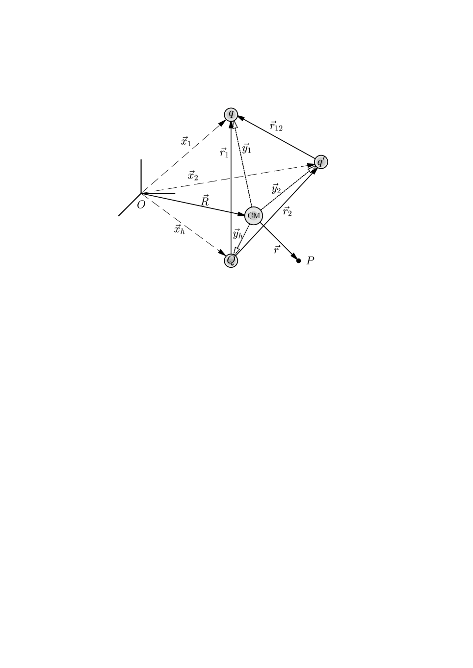
Figure 1: Definition of different coordinates used through this work.

III.1 Intrinsic Hamiltonian

We briefly outline here the procedure followed in Al04 . To separate the Center of Mass (CM) free motion, we went to the heavy quark frame ($\vec{R},\vec{r}_{1},\vec{r}_{2}$), where $\vec{R}$ and $\vec{r}_{1}$ ($\vec{r}_{2}$) are the CM position in the LAB frame and the relative position of the $q$ ($q^{\prime}$) quark with respect to the heavy $Q$ quark. In this frame, the Hamiltonian reads

$$H = -\frac{\vec{\nabla}_{\vec{R}}^{2}}{2M_{\rm tot}}+H^{\rm int}$$ (18)

$$H^{\rm int} = \sum_{i=q,q^{\prime}}h^{sp}_{i}+V_{qq^{\prime}}(\vec{r}_{1}-\vec{r}_{2},spin)-\frac{\vec{\nabla}_{1}\cdot\vec{\nabla}_{2}}{m_{Q}}+\sum_{i=q,q^{\prime},Q}m_{i}$$ (19)

$$h^{sp}_{i} = -\frac{\vec{\nabla}_{i}^{2}}{2\mu_{i}}+V_{Qi}(\vec{r}_{i},spin),\quad i=q,q^{\prime}$$ (20)

where $M_{\rm tot}$ is the sum of quark masses, $\left(m_{q}+m_{q^{\prime}}+m_{Q}\right)$, $\mu_{q,q^{\prime}}=\left(1/m_{q,q^{\prime}}+1/m_{Q}\right)^{-1}$ and $\vec{\nabla}_{1,2}=\partial/\partial_{\vec{r}_{1},\vec{r}_{2}}$. The intrinsic Hamiltonian $H^{\rm int}$ describes the dynamics of the baryon and we used a variational approach to solve it Al02 . $H^{\rm int}$ consists of the sum of two single particle Hamiltonians ($h^{sp}_{i}$), which describe the dynamics of the light quarks in the mean field created by the heavy quark, plus the light–light interaction term, which includes the Hughes-Eckart term ($\vec{\nabla}_{1}\cdot\vec{\nabla}_{2}$). In Ref. Al04 , several quark-quark interactions, fitted to the meson spectra, were used to predict charmed and bottom baryon masses and some static electromagnetic properties. Furthers details can be found there.

III.2 $\Lambda_{b,c}$ and $\Xi_{b,c}$ Wave Functions and HQS

To solve the intrinsic Hamiltonian of Eq. (19), a HQS inspired variational approach was used in Ref. Al04 . HQS is an approximate SU($N_{F}$) symmetry of QCD, being $N_{F}$ the number of heavy flavors. This symmetry appears in systems containing heavy quarks with masses much larger than any other energy scale ($\eta$ = $\Lambda_{QCD}$, $m_{u}$, $m_{d}$, $m_{s}$,…) controlling the dynamics of the remaining degrees of freedom. For baryons containing a heavy quark, and up to corrections of the order ${\cal O}(\frac{\eta}{m_{Q}})$, HQS guarantees that the heavy baryon light degrees of freedom quantum numbers (spin, orbital angular momentum and parity) are always well defined. We took advantage of this fact in Ref. Al04 in choosing the family of variational wave functions. Assuming that the ground states of the baryons are in s–wave and a complete symmetry of the wave function under the exchange of the two light quarks ($u,d,s$) flavor, spin and space degrees of freedom (SU(3) quark model), the wave functions read ($I$, and $S_{\rm light}^{\pi}$ are the isospin, and the spin parity of the light degrees of freedom)

• $\Lambda-$type baryons: $I=0,~{}S_{\rm light}^{\pi}=0^{+}$

  $$|\Lambda_{Q};J=\frac{1}{2},M_{J}\left.\right\rangle = \Big{\{}|00\rangle_{I}\otimes|00\rangle_{S_{\rm light}}\Big{\}}\Psi_{ll}^{\Lambda_{Q}}(r_{1},r_{2},r_{12})\otimes|Q;M_{J}\rangle$$ (21)

  where the spatial wave function, since we are assuming $s-$wave baryons, can only depend on the relative distances $r_{1}$, $r_{2}$ and $r_{12}=|\vec{r}_{1}-\vec{r}_{2}|$. In addition $\Psi_{ll}^{\Lambda_{Q}}(r_{1},r_{2},r_{12})=\Psi_{ll}^{\Lambda_{Q}}(r_{2},r_{1},r_{12})$ to guarantee a complete symmetry of the wave function under the exchange of the two light quarks ($u,d$) flavor, spin and space degrees of freedom. Finally $M_{J}$ is the baryon total angular momentum third component.

• $\Xi-$type baryons: $I=\frac{1}{2},S_{\rm light}^{\pi}=0^{+}$

  $$|\Xi_{Q};J=\frac{1}{2},M_{J};M_{T}\left.\right\rangle = \frac{1}{\sqrt{2}}\Big{\{}|ls\rangle\Psi_{ls}^{\Xi_{Q}}(r_{1},r_{2},r_{12})-|sl\rangle\Psi_{sl}^{\Xi_{Q}}(r_{1},r_{2},r_{12})\Big{\}}\otimes|00\rangle_{S_{\rm light}}\otimes|Q;M_{J}\rangle$$ (23)

  where the isospin third component of the baryon, $M_{T}$, is that of the light quark $l$ ($1/2$ or $-1/2$ for the $u$ or the $d$ quark, respectively).

The spatial wave function, $\Psi_{qq^{\prime}}^{B_{Q}}(r_{1},r_{2},r_{12})$, was determined in Al04 by use of the variational principle $\delta\langle B_{Q}|H^{\rm int}|B_{Q}\rangle=0$, and can be easily reconstructed from Tables X and XI of that reference.

III.3 The $\langle\Lambda_{c};\vec{p}^{\,\prime},s|j_{\mu}^{\rm cc}(0)|\Lambda_{b};\vec{p},r\rangle$ and $\langle\Xi_{c};\vec{p}^{\,\prime},s|j_{\mu}^{\rm cc}(0)|\Xi_{b};\vec{p},r\rangle$ Matrix Elements

We will first focus on the $\Lambda_{b}\to\Lambda_{c}$ matrix element. Within a NRCQM and considering only one–body current operators (spectator approximation) we have in the $\Lambda_{b}$ rest frame

$$\left<\Lambda_{c};\vec{p}\,^{\prime},s|j_{cc}^{\alpha}(0)|\Lambda_{b};\vec{0},r\right> = \sqrt{\frac{E_{\Lambda_{c}}^{\prime}}{m_{\Lambda_{c}}}}\int d^{3}q_{1}d^{3}q_{2}d^{3}q_{h}d^{3}q_{h}^{\prime}\ \sqrt{\frac{m_{b}}{E_{b}(\vec{q}_{h})}}\sqrt{\frac{m_{c}}{E_{c}(\vec{q}_{h}^{\,\prime})}}\Big{[}\bar{u}_{c}^{(s)}(\vec{q}^{\,\prime}_{h})\gamma^{\alpha}(1-\gamma_{5})u_{b}^{(r)}(\vec{q}_{h})\Big{]}$$ (25)

$$\times [\phi^{\Lambda_{c}}_{\vec{p}^{\,\prime}}(\vec{q}_{1},\vec{q}_{2},\vec{q}^{\,\prime}_{h})]^{*}\,\phi^{\Lambda_{b}}_{\vec{0}}(\vec{q}_{1},\vec{q}_{2},\vec{q}_{h})$$

with $\vec{p}^{\,\prime}=\vec{p}-\vec{q}=-\vec{q}$, and $u_{c}$ and $u_{b}$ charm and bottom quark Dirac spinors. The wave functions in momentum space appearing in the above equation are the Fourier transformed of those in coordinate space

$$\phi^{\Lambda_{Q}}_{\vec{P}}(\vec{q}_{1},\vec{q}_{2},\vec{q}_{h})=\int\frac{d^{3}x_{1}}{(2\pi)^{\frac{3}{2}}}\frac{d^{3}x_{2}}{(2\pi)^{\frac{3}{2}}}\frac{d^{3}x_{h}}{(2\pi)^{\frac{3}{2}}}e^{-{\rm i}(\vec{q}_{1}\cdot\vec{x}_{1}+\vec{q}_{2}\cdot\vec{x}_{2}+\vec{q}_{h}\cdot\vec{x}_{h})}\ \psi_{\vec{P}}^{\Lambda_{Q}}(\vec{x}_{1},\vec{x}_{2},\vec{x}_{h})$$ (26)

where the spatial wave function of the $\Lambda_{Q}$ baryon with total momentum $\vec{P}$ (see Eq. (18)) is given by

$$\psi_{\vec{P}}^{\Lambda_{Q}}(\vec{x}_{1},\vec{x}_{2},\vec{x}_{h})=\frac{e^{i\vec{P}\cdot\vec{R}}}{(2\pi)^{\frac{3}{2}}}\Psi^{\Lambda_{Q}}_{ll}(r_{1},r_{2},r_{12})$$ (27)

with $\Psi^{\Lambda_{Q}}_{ll}(r_{1},r_{2},r_{12})$ defined in the previous subsection. The actual calculations are done in coordinate space, and we find

$$\left<\Lambda_{c};-\vec{q},s|j_{cc}^{\alpha}(0)|\Lambda_{b};\vec{0},r\right> = \sqrt{\frac{E_{\Lambda_{c}}^{\prime}}{m_{\Lambda_{c}}}}\int d^{3}r_{1}d^{3}r_{2}\,e^{{\rm i}\vec{q}\cdot\left(m_{q}\vec{r}_{1}+m_{q^{\prime}}\vec{r}_{2}\right)/M_{\rm tot}^{c}}[\Psi^{\Lambda_{c}}_{ll}(r_{1},r_{2},r_{12})]^{*}$$ (28)

$$\times \Big{\{}\sqrt{\frac{m_{b}}{E_{b}(\vec{l}\ )}}\sqrt{\frac{m_{c}}{E_{c}(\vec{l}\,^{\prime})}}\Big{[}\bar{u}_{c}^{(s)}(\vec{l}^{\,\prime})\gamma^{\alpha}(1-\gamma_{5})u_{b}^{(r)}(\vec{l}\ )\Big{]}\Big{\}}\Psi^{\Lambda_{b}}_{ll}(r_{1},r_{2},r_{12})$$

with the operators $\vec{l}={\rm i}\vec{\nabla}_{\vec{r}_{1}}+{\rm i}\vec{\nabla}_{\vec{r}_{2}}$ and $\vec{l}^{\prime}=\vec{l}-\vec{q}$ acting on the $\Lambda_{b}$ intrinsic wave function. Finally, the flavor of the light quarks ($q,q^{\prime}$) are up and down and $M^{c}_{\rm tot}=m_{u}+m_{d}+m_{c}$, with $m_{u}=m_{d}$ as dictated by SU(2)–isospin symmetry.

The $\Xi_{b}\to\Xi_{c}$ matrix element is easily obtained from the results above, by using $\Psi_{ls}^{\Xi_{Q}}$ and $m_{s}$ instead of $\Psi_{ll}^{\Lambda_{Q}}$ and $m_{q^{\prime}}=m_{u}=m_{d}$, respectively.

III.4 Heavy Quark Internal Momentum Expansion and Form Factor Equations

Taking $\vec{q}$ in the positive $z$ direction and by comparing both sides of Eq (28) for the spin flip $\alpha=1~{}{\rm or}~{}2$ and spin non-flip $\alpha=0$ and $\alpha=3$ components, all form factors $F^{\prime}s$ and $G^{\prime}s$ can be found. The main problem lies on the operatorial nature of the right hand side of Eq. (28), which requires of some approximations to make its evaluation feasible. Non relativistic expansions of the involved momenta in Eq. (28) are usually performed HB-NRQM , but this is only justified near $q^{2}_{\rm max}$.

Vector
$\alpha=0$,	spin non–flip	$\hat{F}_{1}+\hat{F}_{2}+\frac{E^{\prime}_{\Lambda_{c}}}{m_{\Lambda_{c}}}\hat{F}_{3}$	=	${\cal I}+\frac{\vec{q}^{\,2}{\cal K}}{2(E_{c}+m_{c})}\left(\frac{m_{c}}{E^{2}_{c}}-\frac{1}{m_{b}}\right)$
$\alpha=3$,	spin non–flip	$\frac{|\vec{q}\,|}{E^{\prime}_{\Lambda_{c}}+m_{\Lambda_{c}}}\hat{F}_{1}+\frac{|\vec{q}\,|}{m_{\Lambda_{c}}}\hat{F}_{3}$	=	$\frac{|\vec{q}\,|{\cal I}}{E_{c}+m_{c}}-\frac{|\vec{q}\,|{\cal K}}{2}\Big{(}\frac{m_{c}}{E_{c}^{2}}+\frac{1}{m_{b}}\Big{)}$
$\alpha=2$,	spin flip	$\frac{|\vec{q}\,|}{E^{\prime}_{\Lambda_{c}}+m_{\Lambda_{c}}}\hat{F}_{1}$	=	$\frac{|\vec{q}\,|{\cal I}}{E_{c}+m_{c}}-\frac{|\vec{q}\,|{\cal K}}{2}\Big{(}\frac{m_{c}}{E_{c}^{2}}-\frac{1}{m_{b}}\Big{)}$
Axial
$\alpha=0$,	spin non–flip	$\frac{|\vec{q}\,|}{E^{\prime}_{\Lambda_{c}}+m_{\Lambda_{c}}}\left(-\hat{G}_{1}+\hat{G}_{2}+\frac{E^{\prime}_{\Lambda_{c}}}{m_{\Lambda_{c}}}\hat{G}_{3}\right)$	=	$-\frac{|\vec{q}\,|{\cal I}}{E_{c}+m_{c}}+\frac{|\vec{q}\,|{\cal K}}{2}\Big{(}\frac{m_{c}}{E_{c}^{2}}+\frac{1}{m_{b}}\Big{)}$
$\alpha=3$,	spin non–flip	$\hat{G}_{1}-\frac{\vec{q}^{\,2}}{m_{\Lambda_{c}}\left(E^{\prime}_{\Lambda_{c}}+m_{\Lambda_{c}}\right)}\hat{G}_{3}$	=	${\cal I}+\frac{\vec{q}^{\,2}{\cal K}}{2(E_{c}+m_{c})}\left(\frac{m_{c}}{E^{2}_{c}}-\frac{1}{m_{b}}\right)$
$\alpha=1$,	spin flip	$\hat{G}_{1}$	=	${\cal I}+\frac{\vec{q}^{\,2}{\cal K}}{2(E_{c}+m_{c})}\left(\frac{m_{c}}{E^{2}_{c}}+\frac{1}{m_{b}}\right)$

Table 1: Equations used to determine the $\Lambda_{b}\to\Lambda_{c}$ transition form factors. The hat form factors and baryon integrals (${\cal I}$ and ${\cal K}$ ) are given in Eqs. (29)–(31).

With the $\Lambda_{b}$ baryon at rest, $\vec{l}$ in Eq. (28) is an internal momentum which is much smaller than any of the heavy quark masses. On the other hand, the transferred momentum $\vec{q}$, which coincides, up to a sign, with the total momentum carried out by the $\Lambda_{c}$ baryon, can be large (note that $|\vec{q}\,|=m_{\Lambda_{c}}\sqrt{w^{2}-1}$ and at $q^{2}=0$, $|\vec{q}\,(w=w_{\rm max})|\approx m_{\Lambda_{b}}/2$). We have expanded the right hand side of Eq. (28), neglecting second order terms in $\vec{l}$, but keeping all orders in $\vec{q}$. For instance, this expansion for the charm quark energy gives: $E_{c}(\vec{l}\,^{\prime})\approx E_{c}(\vec{q}\,)(1-\vec{l}\cdot\vec{q}/E_{c}^{2}(\vec{q}\,))+{\cal O}(\vec{l}^{2}/m_{Q}^{2})$, with $E_{c}(\vec{q}\,)\equiv E_{c}=(m_{c}^{2}+\vec{q}^{\,2})^{1/2}$. Thanks to this novel expansion of the electroweak current operator, in which $\vec{q}$ is exactly treated, we are able to predict the decay distributions for all $q^{2}$ values accessible in the physical decays, improving in this manner on the existing NRCQM calculations. Finally, we get the form factors from two (vector and axial) subsets of three equations with three unknowns ($F^{\prime}s$ and $G^{\prime}s$). For the $\Lambda_{b}\to\Lambda_{c}$ transition, these equations are compiled in Table 1. The hat form factors and the dimensionless baryon integrals (${\cal I}$ and ${\cal K}$ ) appearing in the table are given by

$${\hat{F}}_{i}(w) = \left(\frac{E^{\prime}_{\Lambda_{c}}+m_{\Lambda_{c}}}{2E^{\prime}_{\Lambda_{c}}}\right)^{\frac{1}{2}}\left(\frac{2E_{c}}{E_{c}+m_{c}}\right)^{\frac{1}{2}}F_{i}(w),~{}{\hat{G}}_{i}(w)=\left(\frac{E^{\prime}_{\Lambda_{c}}+m_{\Lambda_{c}}}{2E^{\prime}_{\Lambda_{c}}}\right)^{\frac{1}{2}}\left(\frac{2E_{c}}{E_{c}+m_{c}}\right)^{\frac{1}{2}}G_{i}(w),\quad i=1,2,3$$ (29)

$${\cal I}(w) = \int d^{3}r_{1}d^{3}r_{2}\,e^{{\rm i}\vec{q}\cdot\left(m_{q}\vec{r}_{1}+m_{q^{\prime}}\vec{r}_{2}\right)/M_{\rm tot}^{c}}[\Psi^{\Lambda_{c}}_{ll}(r_{1},r_{2},r_{12})]^{*}\Psi^{\Lambda_{b}}_{ll}(r_{1},r_{2},r_{12})$$ (30)

$${\cal K}(w) = \frac{1}{\vec{q}^{\,\,2}}\int d^{3}r_{1}d^{3}r_{2}\,e^{{\rm i}\vec{q}\cdot\left(m_{q}\vec{r}_{1}+m_{q^{\prime}}\vec{r}_{2}\right)/M_{\rm tot}^{c}}[\Psi^{\Lambda_{c}}_{ll}(r_{1},r_{2},r_{12})]^{*}[\vec{l}\cdot\vec{q}\,]\Psi^{\Lambda_{b}}_{ll}(r_{1},r_{2},r_{12})$$ (31)

For degenerate transitions ($m_{b}=m_{c}=m_{Q}$), the baryon factors ${\cal I}(w)$ and ${\cal K}(w)$ are related, ie $2{\cal K}(w)/{\cal I}(w)=(m_{q}+m_{q^{\prime}})/(m_{q}+m_{q^{\prime}}+m_{Q})$, as can be deduced from a integration by parts in Eq. (31). By means of a partial wave expansion and after a little of Racah algebra, the integrals get substantially simplified. Explicit expressions can be found in the Appendix.

Baryon number conservation implies that $F(1)=\sum_{i}F_{i}(1)=1$ in the limit of equal baryon states. The first equation of Table 1 leads to $\sum_{i}F_{i}(1)={\cal I}(1)$, since $w=1$ implies $|\vec{q}\,|=0$. Besides, ${\cal I}(1)$ accounts for the overlap between the charmed and bottom baryon wave functions and therefore it takes the value 1 for equal baryon states, accomplishing exact baryon number conservation. In general, vector current conservation for degenerate transitions imposes the restriction $F_{2}(w)=F_{3}(w)$, which is violated within the spectator approximation assumed in this work. Thus for instance at zero recoil, we find $F_{2}(1)-F_{3}(1)=1-m_{\Lambda_{Q}}/M_{\rm tot}$, and thus we do not get vector current conservation because of baryon binding terms. Two body currents induced by inter–quark interactions are needed to conserve the vector current.

The corresponding $\Xi_{b}$ decay quantities are obtained from the above expressions by means of the substitutions mentioned at the end of Subsect. III.3. Note that, ${\cal I}$ and ${\cal K}$ depend on both the heavy and light flavors, hence, and for the sake of clarity, from now on we will use the notation ${\cal I}^{cb}_{\Lambda}$ or ${\cal I}^{cb}_{\Xi}$ for the $\Lambda_{b}$ and $\Xi_{b}$ decays , and a similar notation for the ${\cal K}$ factors.

IV HQET and Form Factors

When all energy scales relevant in the problem are much smaller than the heavy quark masses, HQS is an excellent tool to understand charm and bottom physics. Close to zero recoil ($w=1$) and at leading order in the heavy quark mass expansion, only one universal (independent of the heavy flavors) form factor, the Isgur-Wise function ($\xi^{\rm ren}$) is required to describe the $\Lambda_{b}\to\Lambda_{c}$ semileptonic decay. To next order, $1/m_{Q}$, one more universal ($\chi^{\rm ren}$) function and one mass parameter (${\bar{\Lambda}}$) are introduced. These functions, and also the form–factors, depend on the heavy baryon light cloud flavor, and thus in general they will be different for $\Xi-$ transitions, though one expect small deviations thanks to the SU(3)-flavor symmetry.

We compile here some useful results from Ref. HQET2 ; Neubert94 , where more details can be found. Including $1/m_{Q}$ corrections the $\Lambda_{b}\to\Lambda_{c}$ form factors factorize in the form

$$F_{i}(w) = N_{i}(w)\hat{\xi}_{cb}(w)+{\cal O}(1/m_{Q}^{2}),\quad G_{i}(w)=N_{i}^{5}(w)\hat{\xi}_{cb}(w)+{\cal O}(1/m_{Q}^{2}),\qquad i=1,2,3$$ (32)

$$\hat{\xi}_{cb}(w) = \xi^{\rm ren}(w)+\Big{(}\frac{\bar{\Lambda}}{2m_{b}}+\frac{\bar{\Lambda}}{2m_{c}}\Big{)}\left[2\chi^{\rm ren}(w)+\frac{w-1}{w+1}\xi^{\rm ren}(w)\right]$$ (33)

where the coefficients $N_{i},N_{i}^{5}$ contain both radiative ($\hat{C}_{i},\hat{C}^{5}_{i}$) and $1/m_{Q}$ corrections. ${\bar{\Lambda}}$ is the binding energy of the heavy quark in the corresponding $\Lambda$ baryon (${\bar{\Lambda}}=m_{\Lambda_{Q}}-m_{Q}$) and because of the dependence on the heavy quark masses, $\hat{\xi}_{cb}$ is no longer a universal form factor. The function $\chi^{\rm ren}(w)$ arises from higher–dimension operators in the HQET Lagrangian, and vanishes at zero recoil. Both functions $\hat{\xi}_{cb}$ and $\xi^{\rm ren}$ are normalized to one at zero recoil. The numerical values of the correction factors $N_{i},N_{i}^{5}$ depend on the value of $\bar{\Lambda}$, which is not precisely known. We reproduce here (Table 2) Table 4.1 of Ref. HQET2 , where these correction factors are given for all baryon velocity transfer $w$ accessible in the $\Lambda_{b}\to\Lambda_{c}l{\bar{\nu}}_{l}$ decay. The parameters ${\bar{\Lambda}}/2m_{b}$ and ${\bar{\Lambda}}/2m_{c}$ were set to 0.07 and 0.24, respectively. At zero recoil, Luke’s theorem Lu90 protects the quantities $F(w)=\sum_{i}F_{i}(w)$ and $G_{1}(w)$ from ${\cal O}(1/m_{Q})$ corrections

$$F(1)=\sum_{i}F_{i}(1)=\eta_{V}+{\cal O}(1/m_{Q}^{2}),\quad G_{1}(1)=\eta_{A}+{\cal O}(1/m_{Q}^{2})$$ (34)

where $\eta_{V}$ and $\eta_{A}$ are entirely determined by short distance corrections (ie, $N_{1}^{5}(1)=\hat{C}^{5}_{1}(1)$ and $\sum_{i}N_{i}(1)=\sum_{i}\hat{C}_{i}(1)$) which are in principle well known, since they are computed using perturbative QCD techniques. The second relation might be used to extract a model independent (up to $1/m_{Q}^{2}$ corrections) value of $|V_{cb}|$ from the measurement of semileptonic $\Lambda_{b}$ decays near zero recoil, where the rate is governed by the form factor $G_{1}$. From Eq. (6), one finds

$$\lim_{w\to 1}\frac{1}{\sqrt{w^{2}-1}}\frac{{\rm d}\Gamma}{{\rm d}w}=\frac{G^{2}|V_{cb}|^{2}}{4\pi^{3}}m_{\Lambda_{c}}^{3}(m_{\Lambda_{b}}-m_{\Lambda_{c}})^{2}\eta_{A}^{2}+{\cal O}(1/m_{c}^{2})$$ (35)

$w$	$N_{1}$	$N_{2}$	$N_{3}$	$\sum_{i}N_{i}$	$N_{1}^{5}$	$N_{2}^{5}$	$N_{3}^{5}$
1.00	1.49	$-$0.36	$-$0.10	1.03	0.99	$-$0.42	0.15
1.11	1.40	$-$0.32	$-$0.09	0.99	0.94	$-$0.37	0.13
1.22	1.32	$-$0.30	$-$0.09	0.93	0.91	$-$0.34	0.12
1.33	1.26	$-$0.27	$-$0.08	0.91	0.88	$-$0.31	0.11
1.44	1.20	$-$0.25	$-$0.07	0.88	0.85	$-$0.28	0.10

Table 2: Correction factors (taken from Ref. HQET2 ) for the $\Lambda_{b}\to\Lambda_{c}$ decay form factors

V Results

To obtain the wave functions for the $\Lambda_{Q}$ and $\Xi_{Q}$ baryons, we will use different NRCQM interactions whose details can be found in Refs. Al04 . Following the notation of this reference, we will refer to them as AL1, AL1$\chi$, AL2, AP1, AP2 and BD. Their free parameters had been adjusted in the meson sector BD81 ; Si96 ; BFV99 . The potentials considered differ in the form factors used for the hyperfine terms, the power of the confining term ($p=1$, as suggested by lattice QCD calculations GM84 , or $p=2/3$ which for mesons gives the correct asymptotic Regge trajectories Fabre88 ), or the use of a form factor in the One Gluon Exchange (OGE) Coulomb potential Ru75 . All of them provide reasonable and similar masses and static properties for $\Lambda_{Q},\Sigma_{Q},\Sigma^{*}_{Q},\Xi^{\prime},\Xi^{\prime}_{Q},\Xi^{*}_{Q},\Omega_{Q}$ and $\Omega^{*}_{Q}$ baryons Al04 .

For the $\Lambda_{b}-$decay we will pay an special attention to the AL1 and AL1$\chi$ inter–quark potentials. The AL1 potential is based on a phenomenological inter–quark interaction which includes a term with a shape and a color structure determined from the OGE contribution, and a confinement potential. The second model (AL1$\chi$) includes the same heavy quark–light quark potential as the AL1 model, while the light quark–light quark is built from the SU(2) chirally inspired quark-quark interaction of Ref. Fe93 which includes a pattern of spontaneous chiral symmetry breaking, and that was applied with great success to the meson sector in Ref. BFV99 ,

From the experimental side, the $\Lambda_{b}$ semileptonic branching fraction into the exclusive semileptonic mode was measured in DELPHI to be HB-exp

$$Br(\Lambda_{b}^{0}\to\Lambda_{c}^{+}l^{-}{\bar{\nu}}_{l})=\left(5.0^{+1.1}_{-0.8}\,({\rm stat})\,^{+1.6}_{-1.2}({\rm syst})\right)$$ (36)

A remark is in order here, the perturbative QCD corrections have been neglected in Ref. HB-exp , i.e. the correction factors $N_{i},N_{i}^{5}$ are computed with ${\hat{C}}_{1}={\hat{C}}_{1}^{5}=1$ and ${\hat{C}}_{2,3}={\hat{C}}_{2,3}^{5}=0$, and a functional form of the type

$$\hat{\xi}_{cb}(w)=e^{-{\hat{\rho}}^{2}(w-1)}$$ (37)

is also assumed in that reference, where it is also found that

$${\hat{\rho}}^{2}=2.0^{+0.8}_{-1.1}$$ (38)

where all uncertainties quoted in Ref. HB-exp have been added in quadratures. On the other hand, the branching fraction given by the Particle Data Group is pdg04

$$Br(\Lambda_{b}^{0}\to\Lambda_{c}^{+}l^{-}{\bar{\nu}}_{l}+{~{}\rm anything})=\left(9.2\pm 2.1\right)\%$$ (39)

which is hardly consistent to that quoted in Eq. (36). Nevertheless, none of the values quoted in Eqs. (36) and (39) correspond to direct measurements. We will assume here, an error weighted averaged value of those given in Eqs. (36) and (39)

$$\langle Br(\Lambda_{b}^{0}\to\Lambda_{c}^{+}l^{-}{\bar{\nu}}_{l})\rangle_{\rm avg}=\left(6.8\pm 1.3\right)\%$$ (40)

The total $\Lambda_{b}^{0}$ width is given by its lifetime $\tau_{\Lambda_{b}^{0}}=1.229\pm 0.080$ ps pdg04 and thus one finds

$$\Gamma(\Lambda_{b}^{0}\to\Lambda_{c}^{+}l^{-}{\bar{\nu}}_{l})=\left(5.5\pm 1.4\right)10^{10}s^{-1}$$ (41)

Besides, data from $Z$ decays in DELPHI have been searched for ${\bar{\rm B}^{0}_{\rm d}}\to{\rm D}^{*+}l^{-}{\bar{\nu}}_{l}$ decays. These events are used to measure the CKM matrix element $|V_{cb}|$ Exp3

$$|V_{cb}|=0.0414\pm 0.0012\,({\rm stat})\,\pm 0.0021\,({\rm syst})\,\pm 0.0018\,({\rm theory})\,$$ (42)

Let us first examine the bare NRCQM predictions without including HQET constraints.

V.1 NRCQM Form Factors

In Fig. 2 we present the $\Lambda_{b}\to\Lambda_{c}$ form factors obtained from the AL1 inter–quark interaction (left) and also the predictions for the $\hat{\xi}_{cb}$ function (right) as extracted from any of the form factors ($\hat{\xi}_{cb}=F_{i}/N_{i},G_{i}/N_{i}^{5},F/\sum_{i}N_{i},\,i=1,2,3$) shown in the left panel. The correction factors $N_{i},N_{i}^{5}$ are taken from Table 2. Several comments are in order:

• As expected from HQS, the form factors $F_{2}$, $F_{3}$, $G_{2}$ and $G_{3}$ are significantly smaller than the dominant ones $F_{1}$ and $G_{1}$.

• Recalling the discussion of Subsect. III.4 on vector current conservation for degenerate transitions, one must conclude that the NRCQM predictions for the $F_{2}$ and $F_{3}$ form factors are not reliable at all, since their sizes are comparable to the expected theoretical uncertainties, ${\cal O}\left(1-m_{\Lambda_{Q}}/M_{\rm tot}\right)$, affecting them. Presumably, one should draw similar conclusions for the axial $G_{2}$ and $G_{3}$ form factors. As clearly seen in Fig. 2 the $\hat{\xi}_{cb}(w)$ functions obtained from the $F_{2}$, $F_{3}$, $G_{2}$ and $G_{3}$ form factors substantially differ among themselves and are in complete disagreement to those obtained from the $F$ and $G_{1}$ form factors.

• NRCQM predictions for the vector $F$ and axial $G_{1}$ form factors are much more reliable, and lead to similar $\hat{\xi}_{cb}$ functions, with discrepancies smaller than around 4%. Such discrepancies can be attributed either to ${\cal O}(1/m_{Q}^{2})$ corrections, not included in $\hat{\xi}_{cb}$, or to deficiencies of the NRCQM. Lattice results of Ref. HB-Lattice for these two form factors, though have large errors, are in good agreement with the results shown in Fig. 2.

Figure 2: NRCQM $\Lambda_{b}\to\Lambda_{c}$ form factors (left) and $\hat{\xi}_{cb}$ function (right) from the AL1 inter–quark interaction.

V.2 HQET and NRCQM Combined Analysis.

To improve the NRCQM results, we proceed as follows. We assume the NRCQM estimate of the vector form factor $F$ ($F=F_{1}+F_{2}+F_{3}$) to be correct for the whole range of velocity transfers accessible in the physical decay, and use it to obtain the flavor depending $\hat{\xi}_{cb}$ function. Now by using Eq. (32) and the HQET coefficients $N_{i},N_{i}^{5}$ compiled in Table 2, we reconstruct the rest of form factors, in terms of which we can predict the longitudinal and transverse differential decay widths and the asymmetry parameters defined in Subsect. II. We will estimate the theoretical error of the present analysis by accounting for the spread of the results obtained when all calculations are repeated by determining $\hat{\xi}_{cb}$ from the NRCQM $G_{1}$ form factor and/or by using different inter–quark interactions.

V.2.1 $\Lambda_{b}$ Decay

Figure 3: $\Lambda_{b}\to\Lambda_{c}$ form factors (top) and differential decay width (bottom) constrained by means of the HQET relations of Eq. (32). AL1 and AL1$\chi$ inter–quark interactions have been used, and HQET$-F$ and HQET$-G_{1}$ stand for HQET models where $\hat{\xi}_{cb}$ is determined from the NRCQM predictions for the $F$ and $G_{1}$ form factors, respectively. For the AL1+HQET$-F$ model, longitudinal and transverse differential decay distributions are plotted as well. For comparison in the bottom panel, we also show the bare NRCQM decay width distribution obtained from the form factors plotted in the left panel of Fig. 2.

Results of our HQET improved NRCQM analysis for the $\Lambda_{b}$ decay are compiled in Fig. 3 and Tables 3 and 4. In the first of the tables, we give the total and partially integrated semileptonic decay widths, split into the contributions to the rate from transversely $(\Gamma_{T})$ and longitudinally $(\Gamma_{L})$ polarized $W$’s, and the value of the flavor depending $\hat{\xi}_{cb}(w)$ function and its derivatives at zero recoil, together with our estimates for the uncertainties of the present analysis. We also compare, when possible, with the lattice results of Ref. HB-Lattice . In the second of the tables, we compile our predictions for the $w-$averaged asymmetry parameters defined in Eqs. (13)–(16). Our results compare exceptionally well to those obtained by Cardarelli and Simula from a light–front constituent quark model HB-LFQM . On the other hand, we should mention that the NRCQM described in Subsect. V.1 leads to similar (discrepancies of around 2-3%) differential decay rates, as can be appreciated in Fig. 3. From the discussion in Subsect. V.1, this fact should be considered as an accident. For the $w-$averaged asymmetry parameters given in Table 4, discrepancies are in general higher, being of the order of 20% for the $\langle a_{T}\rangle$ and $\langle\alpha^{\prime}\rangle$ asymmetries.

	HQET$-F$	HQET$-G_{1}$	HQET$-F$	HQET$-F$	HQET$-F$	HQET$-F$	HQET$-F$	Theor.	Lattice
	AL1	AL1	AL1$\chi$	AL2	AP1	AP2	BD	Avg.	Ref. HB-Lattice
$\Gamma$	3.46	3.73	3.35	3.57	3.50	3.60	3.49	$3.46^{+0.27}_{-0.11}$	$-$
$\Gamma_{L}$	2.14	2.31	2.07	2.22	2.18	2.25	2.16	$2.14^{+0.17}_{-0.07}$	$-$
$\Gamma_{T}$	1.31	1.42	1.28	1.34	1.33	1.36	1.32	$1.31^{+0.11}_{-0.03}$	$-$
${\hat{\Gamma}}_{L}$, $w_{0}$
1.10	0.23	0.25	0.22	0.22	0.23	0.23	0.23	$0.23^{+0.02}_{-0.01}$	$0.23^{+0.03}_{-0.02}$
1.15	0.43	0.47	0.42	0.43	0.43	0.43	0.43	$0.43^{+0.04}_{-0.01}$	$0.44^{+0.08}_{-0.06}$
1.20	0.68	0.73	0.66	0.69	0.68	0.68	0.68	$0.68^{+0.05}_{-0.02}$	$0.71^{+0.17}_{-0.13}$
1.25	0.96	1.04	0.94	0.98	0.97	0.97	0.96	$0.96^{+0.08}_{-0.02}$	$1.0^{+0.3}_{-0.2}$
1.30	1.26	1.37	1.23	1.29	1.28	1.28	1.27	$1.26^{+0.11}_{-0.03}$	$1.4^{+0.5}_{-0.4}$
1.35	1.59	1.71	1.54	1.63	1.61	1.61	1.60	$1.59^{+0.12}_{-0.05}$	$-$
${\hat{\Gamma}}_{T}$, $w_{0}$
1.10	0.34	0.37	0.34	0.34	0.34	0.34	0.34	$0.34^{+0.03}_{-0.00}$	$0.34^{+0.06}_{-0.04}$
1.15	0.57	0.62	0.56	0.58	0.57	0.57	0.57	$0.57^{+0.05}_{-0.01}$	$0.53^{+0.16}_{-0.14}$
1.20	0.79	0.86	0.78	0.80	0.80	0.80	0.79	$0.79^{+0.07}_{-0.01}$	$0.7^{+0.3}_{-0.3}$
1.25	0.98	1.06	0.96	1.00	0.99	0.99	0.99	$0.98^{+0.08}_{-0.02}$	$0.8^{+0.6}_{-0.5}$
1.30	1.14	1.23	1.11	1.16	1.15	1.15	1.14	$1.14^{+0.09}_{-0.03}$	$0.8^{+0.9}_{-0.8}$
1.35	1.24	1.35	1.22	1.27	1.26	1.26	1.25	$1.24^{+0.11}_{-0.02}$	$-$
$\hat{\xi}_{cb}(1)$	0.97	1.01	0.97	0.97	0.97	0.97	0.97	$0.97^{+0.04}_{-0.00}$	$0.99\pm 0.01$
$-\hat{\xi}_{cb}^{\prime}(1)$	$0.58$	$0.65$	$0.64$	0.52	0.58	0.52	0.56	$0.58^{+0.07}_{-0.06}$	$1.1\pm 1.0$
$-\hat{\xi}_{cb}^{\prime\prime}(1)$	$0.73$	$0.59$	$0.72$	0.79	0.63	0.70	0.82	$0.73^{+0.09}_{-0.14}$	$-$
$\hat{\xi}_{cb}^{\prime\prime\prime}(1)$	2.3	2.0	2.6	2.3	1.8	1.9	2.5	$2.3^{+0.3}_{-0.5}$	$-$

Table 3: $\Lambda_{b}$ semileptonic decay: Theoretical predictions for totally and partially (${\hat{\Gamma}}_{L,T}=\int_{1}^{w_{0}}{\rm d}w\frac{{\rm d}\Gamma_{L,T}}{{\rm d}w}$) integrated decay widths, in units of $|V_{cb}|^{2}10^{13}$ s^-1, and for $\hat{\xi}_{cb}(w)$ and its derivatives at zero recoil. The meaning of columns 2 to 8 is the same as in Fig. 3, with the obvious changes due to the use of different inter–quark interactions. In the ninth column (Theor. Avg.) we give our final results with theoretical uncertainties obtained from the spread of the results shown in the table. Finally in the last column we compile the Lattice QCD results of Ref. HB-Lattice .

	$R_{L/T}$	$\langle a_{T}\rangle$	$\langle a_{L}\rangle$	$\langle P_{L}\rangle$	$\langle\alpha^{\prime}\rangle$	$\langle\alpha^{\prime\prime}\rangle$	$\langle\gamma\rangle$
$\Lambda_{b}^{0}\to\Lambda_{c}^{+}l^{-}{\bar{\nu}}_{l}$	$1.63\pm 0.02$	$-0.665\pm 0.002$	$-0.954\pm 0.001$	$-0.844\pm 0.003$	$-0.156\pm 0.001$	$-0.531\pm 0.004$	$0.439\pm 0.004$
$\Xi_{b}^{0}\to\Xi_{c}^{+}l^{-}{\bar{\nu}}_{l}$	$1.53\pm 0.04$	$-0.628\pm 0.004$	$-0.945\pm 0.002$	$-0.820\pm 0.004$	$-0.154\pm 0.001$	$-0.508\pm 0.008$	$0.475\pm 0.006$

Table 4: Theoretical predictions for the $w-$averaged asymmetry parameters defined in Eqs. (13)–(16). We quote central values from the AL1+HQET$-F$ model and the theoretical uncertainties have been determined as in Table 3.

From our theoretical determination of the total semileptonic width in Table 3 and the experimental estimate in Eq. (41), we get

$$|V_{cb}|=0.040\pm 0.005~{}({\rm stat})~{}^{+0.001}_{-0.002}~{}({\rm theory})$$ (43)

in remarkable agreement with the recent determination of this parameter from ${\bar{\rm B}^{0}_{\rm d}}\to{\rm D}^{*+}l^{-}{\bar{\nu}}_{l}$ decays (Eq. (42)). The experimental uncertainties on the $\Lambda_{b}$ semileptonic branching ratio turn out to be the major source of error in the present determination of $|V_{cb}|$, being the theoretical error in both Eqs. (42) and (43) comparable in size. We point out nevertheless that our determination of $|V_{cb}|$ is based on a NRCQM description of the baryon and as such it is not model independent. From a conceptual point of view a determination of $|V_{cb}|$ based on Eq. (35) would be preferred in a non-relativistic approach as both baryons are at rest in the $w\to 1$ limit. Unfortunately the lack of enough experimental data in that region prevents such a calculation. Note nevertheless that our partially integrated width ($\hat{\Gamma}_{L}+\hat{\Gamma}_{T}$) is in good agreement with the lattice results of Ref. HB-Lattice for $w$ values up to $w\approx 1.20$ ($|\vec{q}\,|\approx 0.66m_{\Lambda_{c}}$) where lattice calculations are reliable, and that our total width $\Gamma=3.46^{+0.27}_{-0.11}\,|V_{cb}|^{2}\,10^{13}$s^-1 agrees with the value of $\Gamma=3.1\pm 1.0\,|V_{cb}|^{2}\,10^{13}$s^-1 obtained in Ref. HB-SR3 using QCD sum rules.

With respect to the $1/m_{Q}-$corrected Isgur-Wise function $\hat{\xi}_{cb}(w)$ our results show a clear departure from a single exponential (see Eq.(37)) functional form, and instead, in the velocity transfer range accessible in the physical decay, it is rather well described by a rank three polynomial in powers of $(w-1)$. In what $\hat{\xi}_{cb}^{\prime}(1)$ respects, our estimate lies in the lower end of the range of Eq. (38). As mentioned above, the perturbative QCD corrections were neglected in Ref. HB-exp . If we do not include the short distance contributions when relating the NRCQM AL1 $F$ form factor and the HQET $\hat{\xi}_{cb}(w)$ function, the slope of this latter function becomes larger (in absolute value), ie $\hat{\xi}_{cb}^{\prime}(1)=-0.99$, in closer agreement with the DELPHI estimate. Besides, the assumption in Ref. HB-exp of the functional form of Eq. (37) leads also to larger, in absolute value, slopes. Thus, to get a semileptonic decay width of 3.46 $|V_{cb}|^{2}10^{13}$s^-1 (our prediction for AL1+HQET-$F$), a value of ${\hat{\rho}}^{2}=1.20$ is required.

Finally, we would like to remark the minor differences, of the order of a few per cent, existing between the AL1 and AL1$\chi$ NRCQM based predictions for the decay distributions. This is a common feature, when the different inter–quark interactions studied in Ref. Al04 are considered. All results are compiled in Table 3.

V.2.2 $\Xi_{b}$ Decay

Figure 4: $\Lambda_{b}\to\Lambda_{c}$ and $\Xi_{b}\to\Xi_{c}$ $1/m_{Q}-$corrected Isgur-Wise functions, $\hat{\xi}_{cb}(w)$, from the AL1+HQET$-F$ model.

	HQET$-F$	HQET$-G_{1}$	HQET$-F$	HQET$-F$	HQET$-F$	HQET$-F$	Theor.	Lattice
	AL1	AL1	AL2	AP1	AP2	BD	Avg.	Ref. HB-Lattice
$\Gamma$	2.96	3.21	3.04	2.97	3.12	3.08	$2.96^{+0.25}_{-0.00}$	$-$
$\Gamma_{L}$	1.79	1.94	1.85	1.80	1.90	1.88	$1.79^{+0.15}_{-0.00}$	$-$
$\Gamma_{T}$	1.17	1.27	1.19	1.17	1.22	1.21	$1.17^{+0.10}_{-0.00}$	$-$
${\hat{\Gamma}}_{L}$, $w_{0}$
1.10	0.27	0.29	0.27	0.27	0.27	0.27	$0.27^{+0.02}_{-0.00}$	$0.28^{+0.02}_{-0.03}$
1.15	0.49	0.54	0.50	0.49	0.50	0.50	$0.49^{+0.05}_{-0.00}$	$0.54^{+0.07}_{-0.08}$
1.20	0.75	0.82	0.76	0.75	0.77	0.77	$0.75^{+0.07}_{-0.00}$	$0.86^{+0.14}_{-0.16}$
1.25	1.03	1.12	1.05	1.03	1.07	1.06	$1.03^{+0.09}_{-0.00}$	$1.2^{+0.2}_{-0.3}$
1.30	1.31	1.42	1.34	1.31	1.37	1.36	$1.31^{+0.11}_{-0.00}$	$1.7^{+0.4}_{-0.4}$
${\hat{\Gamma}}_{T}$, $w_{0}$
1.10	0.39	0.43	0.39	0.39	0.40	0.40	$0.39^{+0.04}_{-0.00}$	$0.38^{+0.05}_{-0.05}$
1.15	0.63	0.68	0.63	0.63	0.64	0.64	$0.63^{+0.05}_{-0.00}$	$0.58^{+0.13}_{-0.15}$
1.20	0.83	0.90	0.84	0.83	0.85	0.85	$0.83^{+0.07}_{-0.00}$	$0.7^{+0.3}_{-0.3}$
1.25	0.99	1.08	1.01	0.99	1.02	1.02	$0.99^{+0.09}_{-0.00}$	$-$
1.30	1.10	1.19	1.12	1.10	1.14	1.13	$1.10^{+0.09}_{-0.00}$	$-$
$\hat{\xi}_{cb}(1)$	0.97	1.01	0.96	0.97	0.97	0.97	$0.97^{+0.04}_{-0.01}$	$0.99\pm 0.01$
$-\hat{\xi}_{cb}^{\prime}(1)$	$1.14$	$1.22$	1.06	1.15	1.02	1.05	$1.14\pm 0.08$	$1.4\pm 0.8$
$-\hat{\xi}_{cb}^{\prime\prime}(1)$	$0.13$	$0.00$	0.30	$0.03$	0.30	0.37	$0.13^{+0.24}_{-0.16}$	$-$
$\hat{\xi}_{cb}^{\prime\prime\prime}(1)$	4.6	4.5	4.7	4.3	4.3	4.7	$4.6^{+0.1}_{-0.3}$	$-$

Table 5: As in Table 3, but for $\Xi_{b}$ baryon semileptonic decay.

Results of our HQET improved NRCQM analysis for the $\Xi_{b}$ decay are compiled in Tables 4 and 5. As in the $\Lambda_{b}-$decay case, the decay parameters do not depend significantly on the potential, among those considered in this work. This fact allows us to make precise theoretical predictions, which nicely agree to the lattice results of Ref. HB-Lattice . On the other hand, we find small SU(3) deviations, and thus as a matter of example we find

$$\frac{\Gamma\left(\Xi_{b}\to\Xi_{c}\,l{\bar{\nu}}_{l}\right)}{\Gamma\left(\Lambda_{b}\to\Lambda_{c}\,l{\bar{\nu}}_{l}\right)}=0.86^{+0.10}_{-0.07},$$ (44)

which will naturally fit within SU(3) symmetry expectations.

Finally, in Fig. 4 we plot the $\Lambda_{b}\to\Lambda_{c}$ and $\Xi_{b}\to\Xi_{c}$ $1/m_{Q}-$corrected Isgur-Wise functions, $\hat{\xi}_{cb}(w)$, from the AL1+HQET$-F$ model. We see there, the size of possible SU(3) symmetry violations as a function of the velocity transfer $w$. The zero recoil slope, in absolute value, is significantly larger for the $\Xi_{b}\to\Xi_{c}$ transition than for the the $\Lambda_{b}\to\Lambda_{c}$ one. A similar behavior is also found in the meson sector in the B$\to{\rm D}_{(s)},{\rm D}^{*}_{(s)}$ decays. Lattice calculations show that the slope at zero recoil of the mesonic Isgur-Wise function is larger in magnitude in the case where the spectator quark is a strange one UKQCD1 .

VI Concluding Remarks

We have identified two of the main deficiencies of the NRCQM description of the semileptonic decay of the $\Lambda_{b}$ and $\Xi_{b}$ baryons: i) A standard momentum expansion of the electroweak current is totally unappropriated, far from the zero recoil point. ii) Within the usual spectator model approximation, with only one–body current operators, the vector part of the electroweak charged current is not conserved for degenerate transitions. Both drawbacks prevent NRCQM’s to make reliable predictions of form factors and totally integrated decay rates. In the present work we have solved both deficiencies, and thus we have developed a novel expansion for the electroweak current operator, where all orders on the transferred momentum $\vec{q}$ are kept. To improve on the second of the mentioned deficiencies, we have also implemented HQET constraints among the form-factors. In addition to other desirable features, we would restore in this way, vector current conservation for degenerate transitions.

Our HQET improved NRCQM analysis leads to an accurate and reliable description of the $\Lambda_{b}$ semileptonic decay. Thus, we determine the $1/m_{Q}-$corrected Isgur-Wise function which governs this process and, thanks to the branching fraction values quoted in Refs. pdg04 and HB-exp , extract the modulus of the $cb$ CKM matrix element (Eq. (43)). Our determination of $|V_{cb}|$ comes out in total agreement with that obtained from semileptonic ${\rm B}\to{\rm D}^{*}$ decays (Eq. (42)), and if it suffers from larger uncertainties that the latter one is because of a poorer experimental measurement of the semileptonic branching fraction for the $\Lambda_{b}$ case. We also give various $w-$averaged asymmetry parameters, which determine the angular distribution of the decay.

In what respects to the $\Xi_{b}-$semileptonic decay, we also find an accurate and reliable description of the various physical magnitudes which govern this transition, and find SU(3) symmetry deviations of the order of 15%. At zero recoil, the $1/m_{Q}-$corrected Isgur-Wise function slope, in absolute value, is significantly larger for the $\Xi_{b}\to\Xi_{c}$ transition than for the the $\Lambda_{b}\to\Lambda_{c}$ one.

Appendix A Evaluation of the ${\cal I}$ and ${\cal K}$ Integrals

We use a partial wave expansion of the $\Lambda_{b}$, $\Lambda_{c}$, $\Xi_{b}$ and $\Xi_{c}$ wave functions,

$$\Psi^{\Lambda_{Q}}_{ll}(r_{1},r_{2},r_{12})=\sum_{l=0}^{+\infty}f^{Q}_{l}(r_{1},r_{2})P_{l}(\mu),\quad\Psi^{\Xi_{Q}}_{ls}(r_{1},r_{2},r_{12})=\sum_{l=0}^{+\infty}g^{Q}_{l}(r_{1},r_{2})P_{l}(\mu),\quad Q=c,b\\$$ (45)

where $\mu$ is the cosine of the angle between the vectors $\vec{r}_{1}$ and $\vec{r}_{2}$, being $r_{12}=(~{}r_{1}^{2}+r_{2}^{2}-2r_{1}r_{2}\mu)^{\frac{1}{2}}$, and $P_{l}$ Legendre polynomials of rank $l$. Therefore, the radial functions $f^{Q}_{l}(r_{1},r_{2})$ and $g^{Q}_{l}(r_{1},r_{2})$ are obtained from their corresponding wave function by means of:

$$f^{Q}_{l}(r_{1},r_{2})=\frac{2l+1}{2}\int_{-1}^{+1}d\mu P_{l}(\mu)\Psi^{\Lambda_{Q}}_{ll}(r_{1},r_{2},r_{12}),\quad g^{Q}_{l}(r_{1},r_{2})=\frac{2l+1}{2}\int_{-1}^{+1}d\mu P_{l}(\mu)\Psi^{\Xi_{Q}}_{ls}(r_{1},r_{2},r_{12})$$ (46)

where $r_{12}$ depend on $r_{1},r_{2}$ and $\mu$. In terms of integrals of the above functions, the baryon factor ${\cal I}^{cb}_{\Lambda}$ reads (we recall that for $\Lambda_{b}$ decay, $|\vec{q}\,|=m_{\Lambda_{c}}\sqrt{w^{2}-1}$),

$${\cal I}^{cb}_{\Lambda}(w) = (4\pi)^{2}\sum_{l}\sum_{l^{\prime}}\sum_{l^{\prime\prime}}(-1)^{l^{\prime\prime}}(ll^{\prime}l^{\prime\prime}|000)^{2}\int_{0}^{+\infty}dr_{1}r_{1}^{2}j_{l^{\prime\prime}}(x_{1})\int_{0}^{+\infty}dr_{2}r_{2}^{2}j_{l^{\prime\prime}}(x_{2})[f^{c}_{l}(r_{1},r_{2})]^{*}f^{b}_{l^{\prime}}(r_{1},r_{2})$$ (47)

where the flavor of the light quarks ($q,q^{\prime}$) are up and down

$$x_{1}=\frac{m_{q}|\vec{q}\,|}{M^{c}_{\rm tot}}r_{1},\quad x_{2}=\frac{m_{q^{\prime}}|\vec{q}\,|}{M^{c}_{\rm tot}}r_{2}$$ (48)

and $M^{c}_{\rm tot}=m_{u}+m_{d}+m_{c}$, with $m_{u}=m_{d}$. Besides, $(ll^{\prime}l^{\prime\prime}|000)$ is a Clebsh-Gordan coefficient and $j_{l}$ are spherical Bessel’s functions.

On the other hand, the baryon factor ${\cal K}$ can be computed as

$${\cal K}^{cb}_{\Lambda}(w) = \frac{16\pi^{2}}{\sqrt{3}|\vec{q}\,|}\sum_{l}\sum_{l^{\prime}}\sum_{l^{\prime\prime}}\sum_{l^{\prime\prime\prime}}\sum_{L=l^{\prime}+1,l^{\prime}-1}(-1)^{l+L}\,{\rm i}^{l^{\prime\prime}+l^{\prime\prime\prime}+1}\Big{(}(2L+1)(2l^{\prime\prime}+1)(2l^{\prime\prime\prime}+1)\Big{)}^{\frac{1}{2}}(lLl^{\prime\prime}|000)$$ (49)

$$\times (l^{\prime}ll^{\prime\prime\prime}|000)(l^{\prime\prime\prime}l^{\prime\prime}1|000)W(l^{\prime\prime\prime}l1L;l^{\prime}l^{\prime\prime})\int_{0}^{+\infty}dr_{1}r_{1}^{2}\int_{0}^{+\infty}dr_{2}r_{2}^{2}\Big{\{}j_{l^{\prime\prime}}(x_{1})j_{l^{\prime\prime\prime}}(x_{2})[f^{c}_{l}(r_{1},r_{2})]^{*}$$

$$\times \Omega_{L}[f^{b}_{l^{\prime}}(r_{1},r_{2})]+j_{l^{\prime\prime}}(\frac{m_{q^{\prime}}}{m_{q}}x_{1})j_{l^{\prime\prime\prime}}(\frac{m_{q}}{m_{q^{\prime}}}x_{2})[f^{c}_{l}(r_{1},r_{2})]^{*}\Omega_{L}[f^{b}_{l^{\prime}}(r_{1},r_{2})]\Big{\}}$$

where $W(...)$ are Racah coefficients, and the differential operators $\Omega_{L}$ are defined as

$$\Omega_{L=l^{\prime}+1}=-\left(\frac{l^{\prime}+1}{2l^{\prime}+1}\right)^{\frac{1}{2}}\left[\frac{\partial}{\partial r_{1}}-\frac{l^{\prime}}{r_{1}}\right],\quad\Omega_{L=l^{\prime}-1}=\left(\frac{l^{\prime}}{2l^{\prime}+1}\right)^{\frac{1}{2}}\left[\frac{\partial}{\partial r_{1}}+\frac{l^{\prime}+1}{r_{1}}\right]$$ (50)

Note that ${\cal K}$ remains finite in the limit $|\vec{q}\,|\to 0$, since one cannot take the orders ($l^{\prime\prime}$ and $l^{\prime\prime\prime}$) of both Bessel functions to be 0 due to the Clebsh-Gordan coefficient $(l^{\prime\prime\prime}l^{\prime\prime}1|000)$. For $\Xi_{b}$ decay, ${\cal I}^{cb}_{\Xi}$ and ${\cal K}^{cb}_{\Xi}$ are obtained from Eqs. (47)–(50), by replacing $f-$type radial wave functions by $g-$type ones and taking $m_{q^{\prime}}=m_{s}$.

Finally, in the $m_{b}>m_{c}>>m_{q},m_{q^{\prime}}$ limit and in the neighborhood of $w=1$, the ${\cal I}$ and ${\cal K}$ baryon factors behave like ${\cal O}(1)$ and ${\cal O}(m_{q}/m_{c},m_{q^{\prime}}/m_{c})$, respectively.

- (1) N. Isgur and M.B. Wise, Phys. Lett. B232 (1989) 292; ibidem Phys. Lett. B237 (1990) 527.
- (2) H. Georgi, Phys. Lett. B240 (1990) 447.
- (3) C.W. Bernard, Y. Shen and A. Soni, Phys. Lett. B317 (1993) 164.
- (4) UKQCD Collaboration, S.P. Booth et al., Phys. Rev. Lett. 72 (1994) 462; K.C. Bowler et al., Phys. Rev. D52 (1995) 5067; ibidem Nucl. Phys. B637 (2002) 293.
- (5) U. Aglietti, G. Martinelli and C.T. Sachrajda, Phys. Lett. B324 (1994) 85; L. Lellouch et al., Nucl. Phys. B444 (1995) 401.
- (6) S. Hashimoto and H. Matsufuru, Phys. Rev. D54 (1996) 4578; S. Hashimoto, et al., Phys. Rev. D61 (2000) 014502.
- (7) M. Neubert, Phys. Rep. 245 (1994) 259.
- (8) A.F. Falk and M. Neubert, Phys. Rev. D47 (1993) 2982; M. Neubert, Phys. Lett. B338 (1994) 84; A. G. Grozin and M. Neubert, Phys. Rev. D55 (1997) 272; M. Neubert, Adv. Ser. Direct. High Energy Phys. 15 (1998) 239; I. Caprini and M. Neubert, Phys. Lett. B380 (1996) 376; I. Caprini, L. Lellouch and M. Neubert, Nucl. Phys. B530 (1998) 153.
- (9) A.F. Falk, E. Jenkins, A.V. Manohar and M.B. Wise, Phys. Rev. D49 (1994) 4553.
- (10) B. Grinstein, M.B. Wise, and N. Isgur, Phys. Rev. Lett. 56 (1986) 298; N. Isgur, D. Scora, B. Grinstein and M.B. Wise, Phys. Rev. D39 (1989) 799; D. Scora and N. Isgur, Phys. Rev. D52 (1995) 2783.
- (11) H. Hogaasen and M. Sadzikowski, Z. Phys. C64 (1994) 427; H.M. Choi and C.R. Ji, Phys. Lett.B460 (1999) 461.
- (12) S. Narison, Phys. Lett. B325 (1994) 197. E. de Rafael and J. Tarón, Phys. Rev. D50 (1994) 373.
- (13) BELLE Collaboration, K. Abe et al., Phys. Lett. B526 (2002) 247
- (14) CLEO Collaboration, J.P. Alexander et al., hep-ex/0007052.
- (15) DELPHI Collaboration, J. Abdallah, Eur. Phys. J. C33 (2004) 213.
- (16) C. Albajar et al., Phys. Lett. B273, 540 (1991).
- (17) S. Eidelman et al., Phys. Lett. B592, 1 (2004).
- (18) DELPHI Collaboration, J. Abdallah, Phys. Lett. B585 (2004) 63.
- (19) UKQCD Collaboration, K.C. Bowler et al., Phys. Rev. D57 (1998) 6948; ibidem Phys. Rev. D54, 3619 (1996).
- (20) S. Gottlieb and S. Tamhankar, Nucl. Phys. B (Proc. Suppl.) 119 (2003) 644.
- (21) E. Jenkins and A. V. Manohar, Nucl. Phys. B396 (1993) 38.
- (22) A.V. Manohar and M.B. Wise, Phys. Rev. D49 (1994) 1310.
- (23) B. Holdom, M. Sutherland and J. Mureika, Phys. Rev. D49 (1994) 2359.
- (24) A. G. Grozin and O. I. Yakovlev, Phys. Lett. B291 (1992) 441.
- (25) R.S. Marques de Carvalho, F.S. Navarra, M. Nielsen, E. Ferreira and H.G. Dosch, Phys. Rev. D60 (1999) 034009.
- (26) C. Jin, Phys. Rev. D56 (1997) 7267.
- (27) M.A. Ivanov, V.E. Lyubovitskij, J. G. Körner and P. Kroll, Phys. Rev. D56 (1997) 348; B. König, J. G. Körner, M. Krämer and P. Kroll, Phys. Rev. D56 (1997) 4282; M.A. Ivanov, J.G. Körner, V.E. Lyubovitskij and A.G. Rusetsky, Phys. Rev. D59 (1999) 074016.
- (28) D. Chakraverty, T. De and B. Dutta-Roy, Mod. Phys. Lett. A12 (1997) 195; D. Chakraverty, T. De, B. Dutta-Roy and K.S. Gupta, Int. J. Mod. Phys. A14 (1999) 2385.
- (29) M. Tanaka, Phys. Rev. D47 (1993) 4969.
- (30) F. Cardarelli and S. Simula, Phys. Lett. B421 (1998) 295; ibidem Phys. Rev. D60 (1999) 074018; ibidem Nucl. Phys. A663 (2000) 931.
- (31) J.P. Lee, C. Liu and H.S. Song, Phys. Rev. D58 (1998) 014013; M.Q. Huang J.P. Lee, C. Liu and H.S. Song, Phys. Lett. B502 (2001) 133; J.P. Lee and G.T. Park, Phys. Lett. B552 (2003) 185.
- (32) I. Dunietz, Phys. Rev. D58 (1998) 094010.
- (33) H.H. Shih, S.C. Lee and H.N. Li, Phys. Rev. D61 (2000) 114002.
- (34) J.G. Körner and B. Melic, Phys. Rev. D62 (2000) 074008.
- (35) N. Isgur and M. B. Wise, Nucl. Phys. B348 (1991) 276; H. Georgi, Nucl. Phys. B348 (1991) 293; T. Mannel, W. Roberts and Z. Ryzak, Nucl. Phys. B355 (1991) 38.
- (36) M.E. Luke, Phys. Lett. B252 (1990) 447.
- (37) H. Georgi, B. Grinstein and M.B. Wise, Phys. Lett. B252 456 (1990); P. Cho and B. Grinstein, Phys. Lett. B285 (1992) 153.
- (38) C. Albertus, J.E. Amaro, E. Hernández and J. Nieves, Nucl. Phys. A740 (2004) 333.
- (39) B. Silvestre-Brac, Few-Body Systems 20 (1996) 1.
- (40) C. Albertus, E. Hernández and J. Nieves, hep-ph/0408065, talk given at ‘BEACH04: 6th International Conference Hyperons, Charm & Beauty hadrons’, Chicago, 2004.
- (41) J.G. Körner and M. Krämer, Phys. Lett. B275 (1992) 495.
- (42) CLEO Collab., M. Bishai et al., Phys. Lett. B350 (1995) 256.
- (43) ARGUS Collab., H. Albrecht et al., Phys. Lett. B274 (1992) 239.
- (44) C. Albertus, J.E. Amaro and J. Nieves, Phys. Rev. Lett. 89, (2002) 032501.
- (45) M. Neubert, Nucl. Phys. B416 (1994) 786.
- (46) R. K. Bhaduri, L.E. Cohler, Y. Nogami, Nuovo Cim. A65 (1981) 376.
- (47) B. Silvestre-Brac, Few-Body Systems 20 (1996) 1.
- (48) L.A. Blanco, F. Fernández and A. Valcarce, Phys. Rev. C59 (1999) 428.
- (49) H. Suganuma, S. Sasaki and H. Toki, Nucl. Phys. B435 (1995) 207.
- (50) F. Gutbrod and I. Montway, Phys. Lett. 136B (1984) 411.
- (51) M. Fabre de la Ripelle, Phys. Lett. 205B (1988) 97.
- (52) A. de Rújula, H. Georgi, and S.L. Glashow, Phys. Rev. D12 (1975) 147.
- (53) F. Fernández, A. Valcarce, U. Straub and A. Faessler, Jour. Phys. G19 (1993) 2013.