Different formulations of ³He and ³H photodisintegration

Abstract

Different momentum space Faddeev-like equations and their solutions for the radiative pd-capture and the three-nucleon photodisintegration of ³He are presented. Applications are based on the AV18 nucleon-nucleon and the Urbana IX three nucleon forces. Meson exchange currents are included using the Siegert theorem. A very good agreement has been found in all cases indicating the reliability of the used numerical methods. Predictions for cross sections and polarization observables in the pd-capture and the complete three nucleon breakup of ³He at different incoming deuteron/photon energies are presented.

I Introduction

In the case of few nucleon systems it is nowadays possible to compare precise experimental data and theoretically well controlled predictions. For low energy processes with three nucleons (3N), theoretical results can be obtained for any given realistic nuclear interaction. This makes such systems an important tool for the investigation of the nuclear Hamiltonian. In momentum space the formalism of Faddeev equations has been used to obtain bound and scattering nuclear states [1]. A very good agreement between theoretical predictions and experimental data was obtained (e.g. [2]). An equivalent description was also obtained using configuration space variational methods [3]. After such encouraging results in pure nucleonic systems had become available also weak and electromagnetic processes with three nucleons were studied in the same scheme. In a series of papers we showed the results for electron induced processes [4], proton-deuteron radiative capture [5], muon capture [6] and 3N bound states photodisintegration [7, 8]. It was found that all dynamical ingredients are important: final state interactions play a significant role and the clear effect of 3N forces is noticed. On top of that also the addition of meson exchange currents changes predictions in a significant way, making the analysis based only on the single nucleon current mostly meaningless. Inclusion of all those components allows for precise predictions on different observables, like cross sections or asymmetries and consequently the door is open for investigations of other physical issues e.g. neutron electromagnetic formfactors [9].

For very low energies hyperspherical harmonic expansion methods were used by the Pisa group [10] and a nice agreement with our results was observed. The total photodisintegration cross sections were also calculated by the Trento group [11] using the Lorentz integral transform method. We compared our results in a common paper [12]. Also the Hanover group presented results on photo- [13] and electro- [14] disintegrations. In their approach the $\Delta$ degree of freedom and corresponding nuclear currents are taken explicitly into account. These predictions are also in qualitative agreement with ours.

In the Faddeev scheme different formulations of the three-body problem are possible. In this work we would like to compare different ways of obtaining transition amplitudes for two- and three- body photodisintegration of 3N bound states. The comparison between predictions based on the different formulations is a strong test of the used numerical methods. The numerical calculation of the three body continuum is a non-trivial problem and the possibility of testing different formulations deserves thorough investigations. Up to now even without 3NF’s, no direct systematic comparison of exclusive three-body photodisintegration cross sections between different approaches was performed. Including 3NF’s the situation is even worse. To the best of our knowledge, no other collaboration has done calculations with explicit 3NF’s. Therefore, an internal comparison is of utmost importance. It also provides useful information on the efficiency of the different formulations for practical calculations.

The calculations presented in this paper are based on the AV18 NN potential [15] alone, and combined with the Urbana IX 3N force [16]. Since the scope of this paper is not an investigation of details of the electromagnetic current operator, the same model of the current is used in all investigated formulations. The single nucleon current is supplemented by some exchange currents included by the Siegert theorem. This approach is described in [5] in more detail.

In Section II we describe three ways of obtaining the transition amplitude for the radiative Nd-capture (and equivalently for the two-body photodisintegration of the 3N bound state) and two methods for the three-body photodisintegration of the 3N bound state. In Section III we compare predictions based on those methods. We summarize in Section IV.

II Theoretical Framework

In this section we would like to describe three different methods used to generate transition amplitudes for the Nd-capture and the two-body photodisintegration of the 3N bound state. We also show how to build the transition amplitudes for the three-body photodisintegration.

The nuclear matrix element for the two-body photodisintegration of the 3N bound state $\mid\Psi_{b}\rangle$ is

$$N^{Nd}_{\mu}\equiv\langle\Psi_{Nd}^{(-)}\mid j_{\mu}\mid\Psi_{b}\rangle\;,$$ (1)

where $\langle\Psi_{Nd}^{(-)}\mid$ is the final scattering state. In the Faddeev scheme it can be presented in the form [7]

$$N^{Nd}_{\mu}=\langle\psi_{1}\mid(1+P)j_{\mu}\mid\Psi_{b}\rangle\;,$$ (2)

where $\langle\psi_{1}\mid$ is a Faddeev component of $\mid\Psi_{Nd}^{(-)}\rangle$ and $j_{\mu}$ is the electromagnetic current operator. $P$ is a permutation operator defined as a sum of cyclical and anti-cyclical permutations of three particles

$$P\equiv P_{12}P_{23}+P_{13}P_{32},$$ (3)

where $P_{ij}$ interchanges the i-th and j-th nucleons.

The Faddeev amplitude $\langle\psi_{1}\mid$ obeys the Faddeev-like equation [17]

$$\langle\psi_{1}\mid = \langle\phi_{1}\mid+\langle\psi_{1}\mid[Pt_{1}G_{0}+(1+P)V_{4}^{(1)}G_{0}(t_{1}G_{0}+1)]$$ (4)

$$\equiv \langle\phi_{1}\mid+\langle\psi_{1}\mid K\;,$$ (5)

where $\mid\phi_{1}\rangle$ is a product of the deuteron state and a momentum eigenstate of the spectator nucleon. Further, $V_{4}^{(1)},G_{0}$ and $t_{1}$ are a part of the 3NF symmetrical under exchanges of nucleons 2 and 3, the free three-nucleon propagator and the two-body t-operator acting in the 2-3 subspace, respectively. Thus

$$\langle\psi_{1}\mid=\langle\phi_{1}\mid(1-K)^{-1}$$ (6)

and

$$N^{Nd}_{\mu}=\langle\phi_{1}\mid(1-K)^{-1}(1+P)j_{\mu}\mid\Psi_{b}\rangle\,.$$ (7)

Defining the auxiliary state $\mid U\rangle$

$$\mid U\rangle\equiv(1-K)^{-1}(1+P)j_{\mu}\mid\Psi_{b}\rangle$$ (8)

one gets

$$N^{Nd}_{\mu}=\langle\phi_{1}\mid U\rangle\;.$$ (9)

According to the definition (8) the state $\mid U\rangle$ fulfills

$$\mid U\rangle=(1+P)j_{\mu}\mid\Psi_{b}\rangle+K\mid U\rangle\;.$$ (10)

Inserting $K$ this reads

$$\mid U\rangle = (1+P)j_{\mu}\mid\Psi_{b}\rangle$$ (11)

$$+ [Pt_{1}G_{0}+(1+P)V_{4}^{(1)}G_{0}(t_{1}G_{0}+1)]\mid U\rangle\;.$$ (12)

This form of the kernel with $P$ standing to the left causes unnecessary complications since the deuteron pole in $t_{1}$ appears as smeared-out into a logarithmic singularity[1]. We avoid that by reformulation of Eq.( 12), as is shown below.

A Methods $1_{NN+3NF}$ and $1_{NN}$

Denoting $\mid\chi\rangle\equiv(1+P)j_{\mu}\mid\Psi_{b}\rangle$ and introducing the auxiliary states $\mid U^{\prime}\rangle$ and $\mid U^{\prime\prime}\rangle$:

$$\mid U^{\prime}\rangle \equiv t_{1}G_{0}\mid U\rangle$$ (13)

$$\mid U^{\prime\prime}\rangle \equiv V_{4}^{(1)}G_{0}(t_{1}G_{0}+1)\mid U\rangle$$ (14)

one gets

$$N^{Nd}_{\mu} = \langle\phi_{1}\mid\chi\rangle+\langle\phi_{1}\mid P\mid U^{\prime}\rangle$$ (15)

$$+ \langle\phi_{1}\mid(1+P)\mid U^{\prime\prime}\rangle\;.$$ (16)

The states $\mid U^{\prime}\rangle$ and $\mid U^{\prime\prime}\rangle$ fulfill the set of coupled equations:

$$\mid U^{\prime}\rangle = t_{1}G_{0}(1+P)j_{\mu}\mid\Psi_{b}\rangle+t_{1}G_{0}P\mid U^{\prime}\rangle$$ (17)

$$+ t_{1}G_{0}(1+P)\mid U^{\prime\prime}\rangle$$ (18)

$$\mid U^{\prime\prime}\rangle = V_{4}^{(1)}G_{0}(1+t_{1}G_{0})\mid(1+P)j_{\mu}\mid\Psi_{b}\rangle$$ (19)

$$+ V_{4}^{(1)}G_{0}(1+t_{1}G_{0})P\mid U^{\prime}\rangle$$ (20)

$$+ V_{4}^{(1)}G_{0}(1+t_{1}G_{0})(1+P)\mid U^{\prime\prime}\rangle\;.$$ (21)

Solving numerically the set of Eqs (18)-(21) and using Eq. (16) one gets the transition amplitude $N^{Nd}_{\mu}$. In the following, the results based on the Eqs (16)-(21) will be denoted as ”method $1_{NN+3NF}$.”

In the case when only the NN interaction is used ($V_{4}^{(1)}=0\Rightarrow\mid U^{\prime\prime}\rangle=0$) Eq. (18) simplifies to

$$\mid U^{\prime}\rangle=t_{1}G_{0}(1+P)j_{\mu}\mid\Psi_{b}\rangle+t_{1}G_{0}P\mid U^{\prime}\rangle$$ (22)

and

$$N^{Nd}_{\mu}=\langle\phi_{1}\mid\chi\rangle+\langle\phi_{1}\mid P\mid U^{\prime}\rangle$$ (23)

This will be called ”method $1_{NN}$.”

In all our methods the inhomogeneous integral equations will always be solved by iteration and consecutive Padé summation. In the numerical implementation it is important that in both methods, during the iterations of the set of Eqs. (18)-(21) or Eq. (22) the permutation operators from the integral kernels act only onto the $t-$operator or the 3NF’s matrix elements, which stand at the very left in the driving terms of Eqs.( 18)-(22). We work in a partial wave decomposition and the presence of the nuclear interactions (in $t_{1}$ and $V_{4}$) enforces that only channels with relatively small partial waves are important. Thus the $P$ operator which acts upon $t_{1}$ or $V_{4}$ can also be taken using a relatively small number of partial waves.

Having solved the set of Eqs. (18)-(21) one can also obtain the amplitude for three-body photodisintegration [7]

$$N^{3N}_{\mu}=\langle\phi_{3N}\mid(1+P)j_{\mu}\mid\Psi_{b}\rangle+\langle\phi_{3N}\mid(1+P)\{\mid U^{\prime}\rangle+\mid U^{\prime\prime}\rangle\}\;.$$ (24)

Here $\langle\phi_{3N}\mid$ is a product of momentum eigenstate describing three free nucleons and antisymmetrized in the 23 subsystem.

B Methods $2_{NN+3NF}$ and $2_{NN}$

The second method, which we will denote as ”$2_{NN+3NF}$” has been presented in detail in [7], where also some predictions for the pd-capture and the two body photodisintegration were shown. However, for the purpose of completeness we briefly describe also this method. Using the identity

$$1+P=\frac{1}{2}P(1+P)$$ (25)

and introducing the auxiliary state $\mid\tilde{U}\rangle$:

$$\mid\tilde{U}\rangle\equiv tG_{0}\mid U\rangle+\frac{1}{2}(1+P)V_{4}^{(1)}G_{0}(tG_{0}+1)\mid U\rangle$$ (26)

one gets from Eq. (12)

$$\mid U\rangle=(1+P)j_{\mu}\mid\Psi_{\rm b}\rangle+P\mid\tilde{U}\rangle\;.$$ (27)

Then the Faddeev-like equation for the state $\mid\tilde{U}\rangle$ is

$$\mid\tilde{U}\rangle = \left(tG_{0}+\frac{1}{2}(1+P)V_{4}^{(1)}G_{0}(tG_{0}+1)\right)$$ (28)

$$* (1+P)j_{\mu}\mid\Psi_{\rm b}\rangle$$ (29)

$$+ (tG_{0}P+\frac{1}{2}(1+P)V_{4}^{(1)}G_{0}(tG_{0}+1)P\mid\tilde{U}\rangle,$$ (30)

and the transition amplitudes are

$$N_{\mu}^{\rm Nd}=\langle\phi_{1}\mid(1+P)\mid j_{\mu}\mid\Psi_{\rm b}\rangle+\langle\phi_{1}\mid P\mid\tilde{U}\rangle$$ (31)

and

$$N_{\mu}^{\rm 3N} = \langle\phi_{3N}\mid(1+P)j_{\mu}\mid\Psi_{\rm b}\rangle$$ (32)

$$+ \langle\phi_{3N}\mid tG_{0}(1+P)j_{\mu}\mid\Psi_{\rm b}\rangle$$ (33)

$$+ \langle\phi_{3N}\mid P\mid\tilde{U}\rangle+\langle\phi_{3N}\mid tG_{0}P\mid\tilde{U}\rangle.$$ (34)

In the case when only the NN interaction is used ($V_{4}^{(1)}=0$) one gets from Eq. (12)

$$\mid U\rangle=\mid\chi\rangle+Pt_{1}G_{0}\mid U\rangle\;.$$ (35)

Using two consequences of the identity (25):
$\mid\chi\rangle=\frac{1}{2}P\mid\chi\rangle$ and $2=P(P-1)$ Eq. (35) can be rewritten as

$$\mid U\rangle=\frac{1}{2}P[\mid\chi\rangle+t_{1}G_{0}P(P-1)\mid U\rangle]\;.$$ (36)

This is equivalent to

$$\mid U\rangle=\frac{1}{2}P\mid U^{\prime\prime\prime}\rangle\;,$$ (37)

where $\mid U^{\prime\prime\prime}\rangle$ fulfills

$$\mid U^{\prime\prime\prime}\rangle=\mid\chi\rangle+t_{1}G_{0}P\mid U^{\prime\prime\prime}\rangle\;.$$ (38)

This equivalence can be easily seen by iterating Eq. (36) and Eq. (38). Therefore one obtains from Eq. (9) and Eq. (37)

$$N^{Nd}_{\mu}=\frac{1}{2}\langle\phi_{1}\mid P\mid U^{\prime\prime\prime}\rangle\;.$$ (39)

The transition amplitude for the three-body photodisintegration is given by [7]

$$N^{3N}_{\mu}=\frac{1}{2}\langle\phi_{3N}\mid P\mid U^{\prime\prime\prime}\rangle+\frac{1}{2}\langle\phi_{3N}\mid tG_{0}P\mid U^{\prime\prime\prime}\rangle\;.$$ (40)

The results based on Eqs. (39) and (40)will be denoted as ”method $2_{NN}$.” In both methods $2_{NN+3NF}$ and $2_{NN}$ one meets the action of the permutation operator P onto matrix elements of the P-operator from the previous iteration. In the actual numerical implementation the identity (25) is fulfilled only approximately. Since we work in a partial wave decomposition, we can take into account only a finite number of partial waves. In order to fulfill the identity (25) a high number of partial waves has to be used. However, also the number of necessary two-body channels increases with the value of total momentum of the two-body subsystem. In consequence, this requires a large amount of memory and computing time. We have found that the worst convergence occurs in the case of method $2_{NN}$ and one needs to use two-body channels with $j_{max}=5$ during the iteration of Eq.( 38). It is due to the lack of the t-matrix in the driving term of this equation. In all other methods the t-matrix, which is most active in the lower channels, reduces the influence of higher two-body channels. Therefore even using the identity (25) one can restrict the number of partial waves.

For all the methods described above, one obtains the transition amplitude $N^{rad}_{\mu}$ for the radiative capture using time reversal in the two-body photodisintegration amplitude $N^{Nd}_{\mu}$.

C Methods $3_{NN+3NF}$ and $3_{NN}$

Another possibility to obtain the transition amplitude $N^{rad}_{\mu}$ is to calculate it directly for the radiative capture process. Then methods used for the elastic Nd scattering can be used where the initial Nd channel state occurs in the driving term of the corresponding equation  [5]. This makes a clear difference to the previous methods. Then the matrix elements of the nuclear current comes in the last stage of the calculations after the solution of the Faddeev equation is obtained.

In this case we calculate directly the transition amplitude for the radiative Nd-capture

$$N^{rad}_{\mu}=\langle\Psi_{b}\mid j_{\mu}\mid\Psi_{Nd}^{(+)}\rangle\;.$$ (41)

The Faddeev component $\mid\psi_{1}\rangle$ forming $\mid\Psi_{Nd}^{(+)}\rangle$ as

$$\mid\Psi_{Nd}^{(+)}\rangle=(1+P)\mid\psi_{1}\rangle$$ (42)

is given via

$$\mid\psi_{1}\rangle=\mid\phi_{1}\rangle+G_{0}\tilde{T}\mid\phi_{1}\rangle\;,$$ (43)

where $\tilde{T}\mid\phi_{1}\rangle$ obeys

$$\tilde{T}\mid\phi_{1}\rangle = tP\mid\phi_{1}\rangle+(1+tG_{0})V_{4}^{(1)}(1+P)\mid\phi_{1}\rangle$$ (44)

$$+ tPG_{0}\tilde{T}\mid\phi_{1}\rangle$$ (45)

$$+ (1+tG_{0})V_{4}^{(1)}(1+P)G_{0}\tilde{T}\mid\phi_{1}\rangle$$ (46)

Solving Eq. (46) one gets the amplitude $\tilde{T}\mid\phi_{1}\rangle$. The next step in the numerical implementation is to apply the free propagator $G_{0}$ and to obtain $\mid\psi_{1}\rangle$. Finally $\langle\Psi_{b}\mid j_{\mu}$ is acted on obtaining the transition amplitude $N^{rad}_{\mu}$. This method we denote by ”method $3_{NN+3NF}$.”

In the absence of the 3N force Eq. (46) simplifies to

$$\tilde{T}\mid\phi_{1}\rangle=tP\mid\phi_{1}\rangle+tPG_{0}\tilde{T}\mid\phi_{1}\rangle$$ (47)

and the corresponding result will be denoted as ”$3_{NN}$.” In our numerical implementation we always calculate the matrix elements of the current operator in the frame in which the photon momentum is parallel to $z$-axis. To obtain the transition amplitude for each final angle between the outgoing photon and the beam direction we have to adjust the corresponding initial deuteron or proton beam direction. This demands the repetition of the iteration of Eq. (46) in each case. One can avoid this by calculating the matrix elements of the current operator in a general frame.

Of course, the methods $3_{NN+3NF}$ and $3_{NN}$ by construction can be used only for the Nd-radiative capture and the two-body photodisintegration.

III Results

We would like to present the quality of our methods for pd-capture for six exemplifying observables: the nucleon and deuteron vector analyzing powers $A_{Y}(N)$ and $A_{Y}(d)$, the differential cross sections and the tensor analyzing powers $A_{YY}$, $A_{XX}$ and $T_{21}\equiv\frac{-1}{\sqrt{3}}A_{XZ}$.

Predictions based on the AV18 interaction for these observables for pd capture are presented in Fig. 1. The incoming deuteron laboratory energy is $E_{d}=300$ MeV. This is equivalent to a photon laboratory energy $E_{\gamma}\approx$106 MeV in the photodisintegration process. The iteration of the Faddeev-like equations uses a lot of computer power. Thus in the case of method $3_{NN}$ which in our numerical implementation, as mentioned above, demands a separate solution of Eq.( 47) for each angle of the outgoing photon we present only a few points (denoted by crosses). We see that the methods $1_{NN}$ and $3_{NN}$ agree nicely in all cases, except for the tensor analyzing power $A_{XX}$ at small angles. This agreement is obtained taking into account in both methods the partial waves with total angular momenta in the two-body subsystem up to $j=3$. The method $2_{NN}$ demands much more partial waves (up to $j=5$) and still there are more angular ranges where the predictions of method $2_{NN}$ differ from those of methods $1_{NN}$ and $3_{NN}$. As mentioned above this is due to the lack of the t-matrix in the driving term.

A nice agreement is obtained when comparing results of methods $1_{NN+3NF}$, $2_{NN+3NF}$ and $3_{NN+3NF}$. This is shown in Fig. 2 for the same deuteron energy, E_d=300 MeV, and for a much lower one, E_d=17.5 MeV, in Fig. 3. The cross section is especially insensitive to the used method. In addition to predictions based on the AV18 and the Urbana IX forces in Figs. 2 and  3 we present also results based on the AV18 interaction alone. As we see, except for the cross section, the three nucleon force effects are very small. Comparison to the Sagara data [18] at E_d=17.5 MeV shows a reasonable agreement for the tensor analyzing powers $A_{XX}$ and $A_{YY}$ and the known disagreement for vector analyzing power $A_{Y}(d)$ [5]. Comparing our predictions to the Pickar data [19] at E_d=300 MeV we see that for the proton analyzing power $A_{Y}(N)$ we agree with the data at the lower and middle angles, while at the higher angles all theoretical predictions are above the data. In the case of the cross section differences are much smaller, however the theoretical predictions seem to be flatter than data. It is also very apparent that the inclusion of the Urbana IX 3NF improves the description of the data. Only two experimental points at very small and at very large angles are in better agreement with the pure NN force prediction.

As is well known, for low energies the 3NF contributes mainly in the 3N bound state, while for higher energies the 3NF effects are seen also in the continuum. This is the reason why we present results also for a relatively high energy (E_d=300 MeV). We also note that the agreement between all three methods is slightly better for lower energy, especially for the deuteron tensor analyzing powers (e.g. A_XX).

The next two figures show dependences of our results on the number of partial waves for the example of method $1_{NN+3NF}$. In Fig. 4 we show the convergence of the predictions in the total angular momentum $J_{max}$ of the three-body system. While using only channels with $J_{max}=\frac{3}{2}$ is absolutely insufficient, using channels with $J_{max}=\frac{7}{2}$ is very close to the final prediction with $J_{max}=\frac{15}{2}$. Allowing the transitions to higher total angular momenta states (up to $J_{max}=\frac{19}{2}$) does not change the predictions in a perceptible manner. A similar picture appears for the convergence in the number of partial waves used in the two-body subsystem (see Fig. 5). While using only channels with total angular momenta in the two-body subsystem up to $j=2$ is far from the predictions with $j=4$, there is only a small difference between the predictions with maximal values of the two-body total angular momentum $j=3$ and $j=4$. However, the method $2_{NN}$ (not shown in Fig. 5) requires at least $j_{max}=5$.

Finally, we would like to compare predictions for the three-body photodisintegration of ³He. In Figs. 6-9 we present examples of exclusive differential cross sections for different kinematical configurations at E_γ=100 MeV, given as a function of the S-curve arc-length. The two protons are measured under different polar and azimuthal angles $\Theta$, $\Phi$. In all cases we see that there is an excellent agreement between the predictions based on methods $1_{NN+3NF}$ and $2_{NN+3NF}$. They are represented by solid and thick dotted curves, respectively. In both cases we show results with channels up to $j_{\max}\leq 3$ and $J_{\max}\leq\frac{15}{2}$. As we checked for a large number of configurations (about 300 000) the differences remain for all cases below 1%. In the case of the predictions based on NN interaction only, the differences are a bit bigger - for the majority of the configurations they are below 5%. In that case channels with $j_{\max}\leq 4$ were used for the method $1_{NN}$ (dotted line) and with $j_{\max}\leq 5$ for the method $2_{NN}$ (dashed line). Again, the reason are the different forms of the driving term in the two methods.

IV Summary

Different formulations of Faddeev-like equations for pd-capture (equivalent to two-body photodisintegration of the 3N bound state) and for three-body photodisintegration of the 3N bound state have been investigated. This is important to guarantee reliable and well converged theoretical results for modern NN and 3N forces. Such tools allow an unambiguous test of the dynamics when compared to data. This study is especially timely since a new approach to nuclear forces and currents based on effective field theory constrained by chiral symmetry is under vivid development [20] -[21]. As we demonstrated all methods show a good agreement. Also the computer time needed is very similar. Therefore, none of them is preferable, but all are equally useful. The comparison, however, was a very important internal benchmark of the methods. Only the method $2_{NN}$ is much slower, since there more two-body partial waves have to be used. For that reason we have not checked another fourth possible formulation with the same driving term as in the method $2_{NN}$, but also three nucleon interaction in the integral kernel [7]. The reason for the slow convergence is that the permutation operator from the integral kernel acts onto the permutation operator from the driving term and one has to use a much bigger number of partial waves to obtain converged results.

We can conclude that now different methods are available, which can be considered to be very reliable and the achieved results document the numerical accuracy up to the order of a few percent slightly dependent on the observable. At the low energies the accuracy is much better. In addition this can be improved if smaller experimental errors in the future will require that.

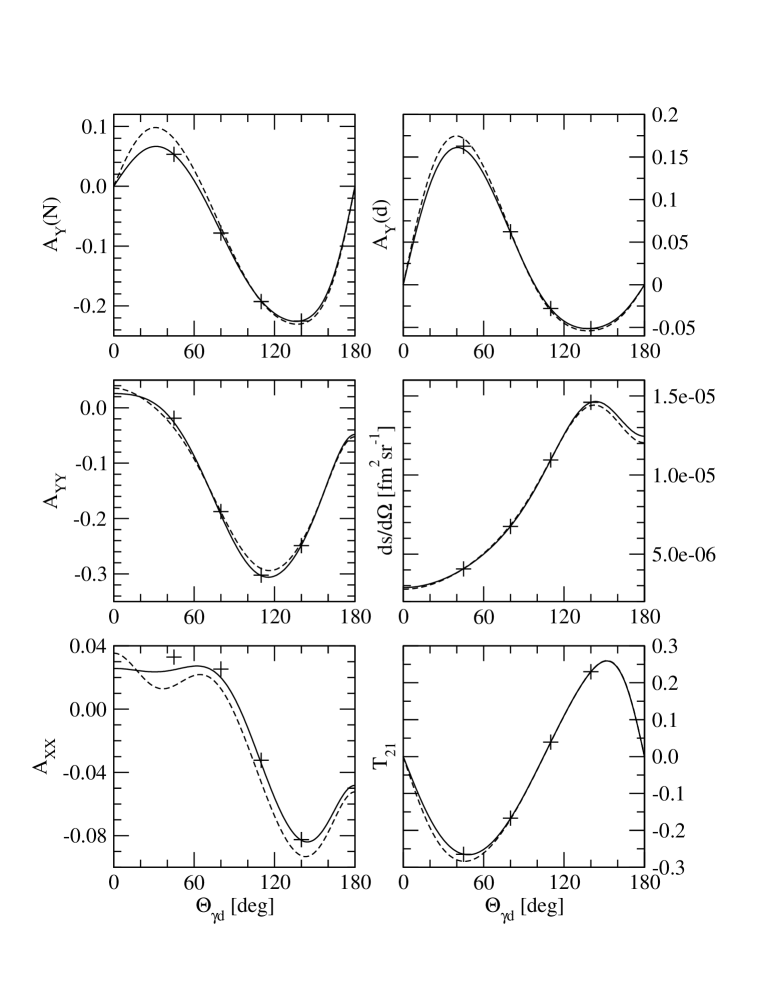
FIG. 1.: The comparison of the three methods using the AV18 interaction at the deuteron laboratory energy E_d=300 MeV. The solid line represent predictions based on method $1_{NN}$, the dashed one on method $2_{NN}$ (here j_max=5) and the crosses are for method $3_{NN}$ (see text).

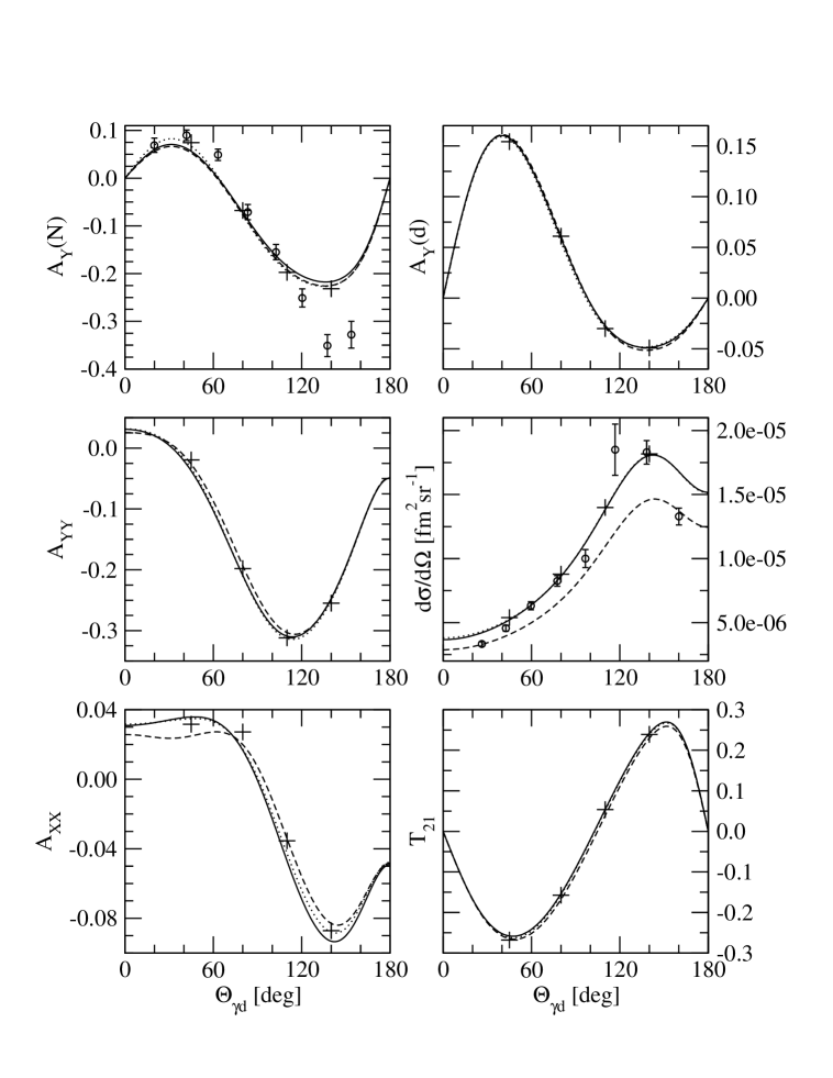
FIG. 2.: The comparison of the three methods using the AV18+UrbanaIX interaction at the deuteron laboratory energy E_d=300 MeV, j_max=3, J${}_{\rm max}=\frac{15}{2}$. The solid line represent predictions based on method $1_{NN+3NF}$, the dotted one on method $2_{NN+3NF}$ and the crosses are for method $3_{NN+3NF}$. The dashed line represents predictions of method $1_{NN}$, based only on the AV18 interaction. Data ($\circ$) are from [19].

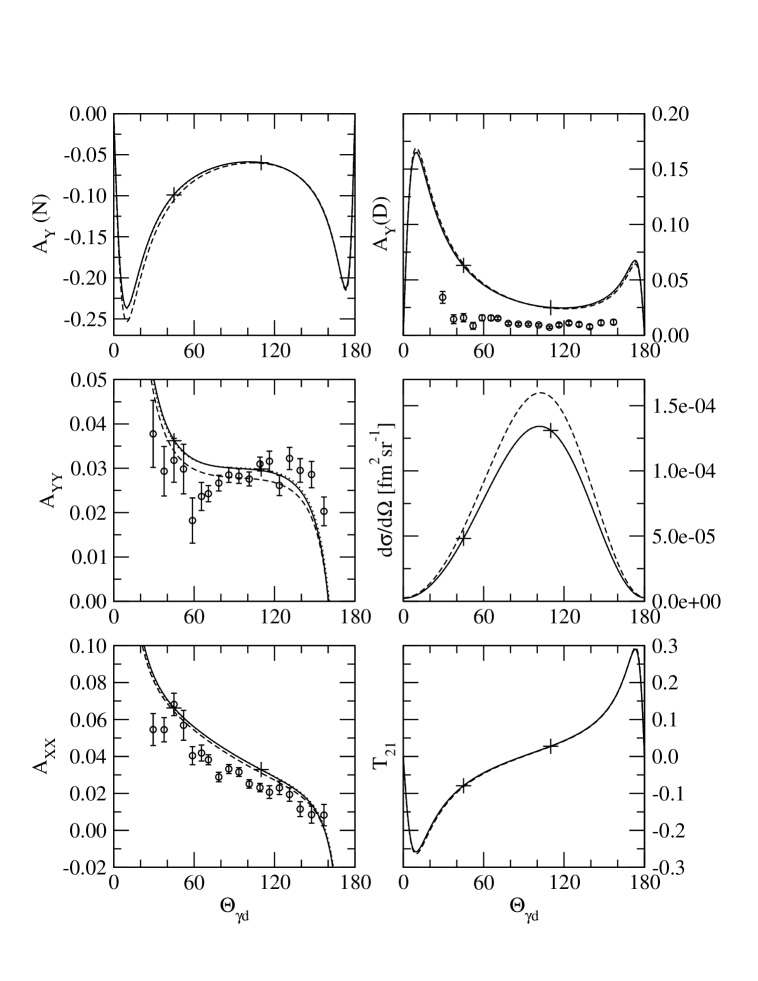
FIG. 3.: The comparison of the three methods using the AV18+UrbanaIX interaction at the deuteron laboratory energy E_d=17.5 MeV, j_max=3, J${}_{\rm max}=\frac{15}{2}$. Curves and crosses as in Fig. 2. Data ($\circ$) are from [18].

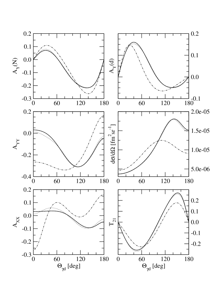
FIG. 4.: The convergence in the number of three-body partial waves for the method $1_{NN+3NF}$ using the AV18+UrbanaIX interaction. E_d=300 MeV, j_max=3 fixed, J${}_{\rm max}=\frac{3}{2}$ (dash-dotted),$\frac{7}{2}$ (dotted),$\frac{15}{2}$ (dashed), $\frac{19}{2}$ (solid line). Dashed and solid lines are indistinguishable.

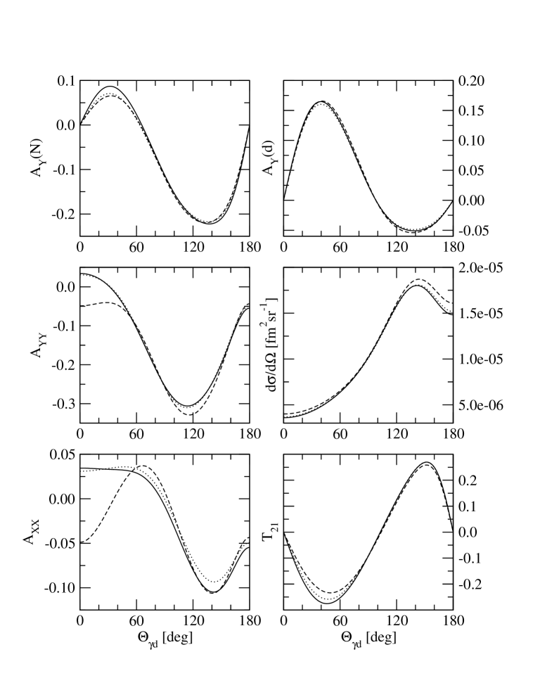
FIG. 5.: The convergence in the number of two-body partial waves for method $1_{NN+3NF}$ using the AV18+UrbanaIX interaction. E_d=300 MeV, J_max=$\frac{15}{2}$ fixed, j${}_{\rm max}=2$ (dashed), 3 (dotted) and 4 (solid line).

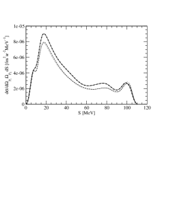
FIG. 6.: The differential cross section for three-body photodisintegration at E_γ=100 MeV at the two proton angles: $\Theta_{1}=10^{\circ}$, $\Phi_{1}=0^{\circ}$, $\Theta_{2}=10^{\circ}$, $\Phi_{2}=0^{\circ}$. The dotted, dashed, solid and thick dotted curves represent methods $1_{NN}$, $2_{NN}$, $1_{NN+3NF}$, $2_{NN+3NF}$, respectively.

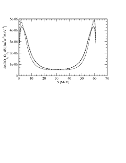
FIG. 7.: The differential cross section for three-body photodisintegration at E_γ=100 MeV at protons angles: $\Theta_{1}=90^{\circ}$, $\Phi_{1}=0^{\circ}$, $\Theta_{2}=90^{\circ}$, $\Phi_{2}=90^{\circ}$. Curves as in Fig. 6.

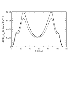
FIG. 8.: The differential cross section for three-body photodisintegration at E_γ=100 MeV at protons angles: $\Theta_{1}=90^{\circ}$, $\Phi_{1}=0^{\circ}$, $\Theta_{2}=90^{\circ}$, $\Phi_{2}=180^{\circ}$. Curves as in Fig. 6.

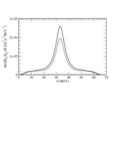
FIG. 9.: The differential cross section for three-body photodisintegration at E_γ=100 MeV at protons angles: $\Theta_{1}=90^{\circ}$, $\Phi_{1}=55^{\circ}$, $\Theta_{2}=90^{\circ}$, $\Phi_{2}=65^{\circ}$. Curves as in Fig. 6.

- [1] W. Glöckle, H. Witała, D. Hüber, H. Kamada and J. Golak, Phys. Rep. 274, (1996) 107.
- [2] St.Kistryn et al.: Phys. Rev. C68, (2003) 054004.
- [3] A.Kievsky, M.Viviani and S.Rosati, Phys. Rev. C64, (2001) 024002; A.Kievsky, M.Viviani and L.Marcucci, Phys. Rev. C69, (2004) 014001; A.Kievsky et al., Phys.Rev. C58, (1998) 3085.
- [4] J. Golak et al. Phys. Rev. C51, (1995) 1638.
- [5] J. Golak et al., Phys. Rev. C62, (2000) 054005.
- [6] R.Skibiński et al.: Phys. Rev. C59, (1999) 2384.
- [7] Skibiński R, Golak J, Kamada H, Witała H, Glöckle W, Nogga A, Phys. Rev. C67, (2003) 054001.
- [8] Skibiński R, Golak J, Kamada H, Witała H, Glöckle W, Nogga A, Phys. Rev. C67, (2003) 054002.
- [9] W.Xu et al: Phys. Rev. Lett. 85, (2000) 2900.
- [10] M.Viviani et al.: Phys. Rev. C61, (2000) 064001.
- [11] V.Efros, W.Leidemann, G.Orlandini, E.Tomusiak: Phys. Lett. B484, (2000) 223.
- [12] Golak J, et al.: Nucl. Phys. A707, (2002) 365.
- [13] L.P. Yuan et al.: Phys. Rev. C66, (2002) 54004; A.Deltuva et al.: Phys. Rev. C69, (2004) 034004.
- [14] A.Deltuva et al.: nucl-th/0406065, to be published in Phys. Rev. C.
- [15] R. B. Wiringa, V.G.J. Stoks, and R. Schiavilla, Phys. Rev. C51, (1995) 38.
- [16] B. S. Pudliner, V. R. Pandharipande, J. Carlson, Steven C. Pieper, and R. B. Wiringa, Phys. Rev. C56, (1997) 1720.
- [17] D. Hüber, H.Kamada, H.Witała, W.Glöckle, Acta Phys. Pol. B28, (1997) 189.
- [18] H. Akiyoshi et al.: Phys. Rev. C64, (2001) 034001.
- [19] M. A. Pickar et al.: Phys. Rev. C35 (1987) 37.
- [20] E.Epelbaum et al.: nucl-th/0405048, to be published in Nucl. Phys. A.
- [21] T-S. Park, D-P. Min, M.Rho, Nucl. Phys. A596, (1996) 515.