Coulomb breakup effects on the optical potentials of weakly bound nuclei

Abstract

The optical potential of halo and weakly bound nuclei has a long range part due to the coupling to breakup that damps the elastic scattering angular distributions. In order to describe correctly the breakup channel in the case of scattering on a heavy target, core recoil effects have to be taken into account. We show here that core recoil and nuclear breakup of the valence nucleon can be consistently taken into account. A microscopic absorptive potential is obtained within a semiclassical approach and its characteristics can be understood in terms of the properties of the halo wave function and of the reaction mechanism. Results for the case of medium to high energy reactions are presented.

1 Introduction

Since the advent of Rare Isotope Beams (RIBs) [1] elastic nucleus-nucleus scattering with a radioactive projectile [2] is a reaction which has been studied to a large extent in the attempt to find characteristics that would be typical for a weakly bound nucleus and would help understanding new phenomena such as the existence of the halos [3]. It has been established that for halo projectiles breakup of the valence particles is responsible for a damping in the elastic angular distribution starting from around 5^o at medium to high energies.

All theoretical methods used to describe the above mentioned reactions, require at some stage of the calculation the knowledge of the nucleus-nucleus optical potential. The optical potential is the basic ingredient for the description of elastic scattering, but it is important also in transfer and breakup calculations, since one needs to take into account the core quasi-elastic scattering by the target while the valence neutrons are transferred or breakup. For example in the case of some two-neutron halo nuclei such as ¹⁴Be or ¹¹Li, their cores of ¹²Be and ⁹Li are themselves weakly bound nuclei. For multinucleon transfer reactions planned in order to obtain heavy exotic nuclei it will be important to have the appropriate optical potentials which include breakup and which should be used in the intermediate steps of the reaction. In the charge exchange reaction ${}^{11}B(^{7}Li,^{7}Be)^{11}Be$ the halo nucleus-nucleus optical potential necessary to describe the final channel [4] has a volume part obtained with a double folding plus a very diffuse surface term fitted phenomenologically to reproduce the final channel angular distribution. The effect of the surface potential reduced the absolute cross sections by about 50%[4], in accordance with the experimental data and it can be interpreted as due to the halo breakup.

Microscopic optical potentials for a halo projectile have already been studied by many authors, and a review of the present situation can be found in [5, 6]. One of these methods consists in starting from a phenomenologically determined core-target potential and then to add the effect of the breakup of the halo neutron. This process leads to adding a surface part to the core-target potential. This new surface peaked optical potential has been seen to have a quite long range which reflects the properties of the long tail of the halo neutron wave function. Such kind of potentials are often called dynamical polarization potentials [6]-[17].

In a recent contribution we proposed a new approach [5] to the calculation of the imaginary part of the optical potential due to nuclear breakup. It is based on a semiclassical method described by Broglia and Winther in [18, 19] and used also by Brink and collaborators [20, 21] to calculate the surface optical potential due to transfer and on the Bonaccorso and Brink model for transfer to the continuum reactions [22]-[26], the idea being that breakup is a reaction following the same dynamics as transfer but leading mainly to continuum final states when the incident energies per nucleon are higher than the average nucleon binding energy. The calculations were almost completely analytical and a simple, approximated formula was obtained which helped understanding the origin of the long range nature of the potential and its dependence on the incident energy as well as on the initial neutron binding energy. The characteristics of our potential were consistent with those of potentials obtained with other methods, in particular the eikonal method of Canto et al.[10] and application to the description of experimental data were encouraging [5].

However it is very well known that for heavy targets recoil effects which give rise to the so called Coulomb breakup, are important and actually dominant for a neutron halo [28, 29, 30, 31] in the breakup cross section and therefore one wonders what would be their effect on the elastic scattering. Some work has already been published in order to calculate the optical potential due to Coulomb breakup at low [14],[15] or intermediate energies [27, 28]. However paper [28] deals with proton halo breakup which, as it has been demostrated in Ref.[29] has to be treated with great care when compared to neutron breakup. Therefore the methods used in [28] to include breakup in the optical potential are not expected to be applicable to the neutron breakup case. We will show in this paper that the method used in Ref.[5] can be used in the case of Coulomb breakup as well and that the corresponding formalism, which is appropriate to reactions performed at medium to high energies, well above the Coulomb barrier, is consistent with and joins continuously to the formalism used by other authors [14] at lower energies.

2 Theory

The method we use here is the same as in [5] and it is based on the extraction of an optical potential from the calculation of a phase shift.

The elastic scattering probability is $P_{el}=|S_{NN}|^{2}$, given in terms of the nucleus-nucleus S-matrix. We know that

$$|S_{NN}(b)|^{2}=e^{-4\delta_{I}(b)}.$$ (1)

In a semiclassical approximation [18], the imaginary part of the nucleus-nucleus phase shift $\delta_{I}$ is related to the imaginary part of the optical potential by

$$\delta_{I}(b)=-{1\over 2\hbar}\int_{-\infty}^{+\infty}\left(W_{V}({\bf r}(t))+W_{S}({\bf r}(t))\right)dt$$ (2)

where the volume potential is responsible for the usual inelastic core-target interaction, while the surface term takes care of the peripheral reactions like transfer and breakup. ${\bf r}(t)={\bf b_{c}}+vt$ is the classical trajectory of relative motion for the nucleus-nucleus collision.

According to [5] the surface optical potential $W_{S}({\bf r}(t))$ due to breakup can be related to the breakup probability by

$$\int_{-\infty}^{+\infty}W_{S}({\bf r}(t))dt=-{\hbar\over 2}P_{b_{up}}(b_{c})$$ (3)

where $P_{b_{up}}=\sum_{i}p_{i}$ are the breakup probabilities in the various channels $i$. In order to obtain the surface imaginary potential Eq. (3) should be calculated as an identity in the distance of closest approach, which amounts to require that $W_{S}(r)$ be a local, angular momentum independent function. We remind the reader that since we are using a semiclassical method, the non locality, which is in principle a characteristic of microscopic optical potentials has been transformed into an energy dependence [35].

Eq.(3) can also be derived in a straightforward way from the time dependent scattering Schrödinger equation for the elastic channel probability density function in presence of a complex potential [21, 32]. In the traditional formulation the index (i) stands for stripping and pickup to bound states and in Ref.[5] we extended it to hold for breakup reactions in which the final neutron state is in the continuum. Nuclear breakup of both absorptive and diffractive type was included and here we will include also Coulomb breakup. The justification of the use of Eq.(3) to calculate the imaginary potential due to nuclear breakup was simply given by the analogy between breakup and transfer as expressed by the transfer to the continuum model introduced in Refs.[22]-[26]. There it was shown that the formalism for transfer to bound states goes over transfer to the continuum in a natural way if the kinematics of the reaction is taken into account correctly within a time dependent approach which ensures neutron energy conservation.

On the other hand Broglia and Winter in [18, 19] pointed out the fact that the same formalism could be extended to include core recoil. In the case of breakup of weakly bound nuclei we have shown in Ref.[33, 34] that core recoil is responsible for the Coulomb breakup and that nuclear and Coulomb breakup give rise to negligible interference effects. Therefore we argue here that the imaginary part of the optical potential due to Coulomb breakup can also be calculated by Eq.(3) where now one of the $p_{i}$ probabilities will be that of Coulomb breakup of the valence nucleon.

Then, using Eq.(2) and (3), in (1) the nucleus-nucleus S-matrix, in the case of a halo projectile, can be written as

$$|S_{NN}|^{2}=|S_{CT}|^{2}e^{-P_{b_{up}}}$$ (4)

where $S_{CT}$ takes into account all core-target interactions while the term $e^{-P_{b_{up}}}$ depends only on the halo neutron breakup probability. For a halo nucleus at high incident energy the transfer probability is going to be much smaller than the breakup probability, therefore the surface potential has been identified here with the breakup potential.

Now we discuss the hypothesis leading to Eq.(4). They have been already discussed in Ref.[5] but we report them here too for the sake of completness.

In this paper we are concerned with reactions performed at energies well above the Coulomb barrier where many inelastic channels open at about the same distance of closest approach. The effect of the breakup is most important at large distances of closest approach ($b_{c}>R_{s}$), where it represents the dominant reaction mechanism. If the breakup probability is needed at smaller impact parameters, then the values calculated by perturbation theory, have to be multiplied by the core survival probability, as discussed in Eq.(V.8.1) of Broglia and Winther and also used in relation to halo breakup by several authors. The effect of all inelastic channels $n$ different from the one we are interested in, can be taken into account by introducing a damping factor $P_{0}$. Therefore the breakup probability $P_{b_{up}}$ at all distances can be defined as

$$P_{b_{up}}=p_{b_{up}}\prod_{n}(1-p_{n})\approx p_{b_{up}}\exp(-\sum_{n}p_{n})=p_{b_{up}}P_{0}$$ (5)

Each elementary inelastic probability $p_{n}$ and breakup probability $p_{b_{up}}$ is small and $p_{b_{up}}$ in particular, can be calculated in time dependent perturbation theory, as done in [22]. In reactions with halo projectiles the damping factor $P_{0}$ has also been referred to as the core survival probability after the halo breakup or as the core elastic scattering probability. The breakup probability Eq.(5) integrated over the core-target impact parameter $b_{c}$ has been widely used in the literature to get breakup cross sections.

In this paper we will treat both nuclear and Coulomb breakup as independent process with the formalism used in Ref.[33], namely we will calculate nuclear breakup in the eikonal approximation and Coulomb breakup in first order perturbation theory. In Ref.[33, 34] we showed that this is appropriate for a one neutron halo since the interference effects are small and the higher order effects in Coulomb breakup are negligible. This has been confirmed by recent experimental data [31]. The case of a proton halo or a two-neutron halo might need the full all-order approach.

Then the total breakup probability will be given by

$${p_{b_{up}}(b_{c})}=p^{N}_{b_{up}}(b_{c})+p^{C}_{b_{up}}(b_{c}).$$ (6)

2.1 Nuclear breakup

The optical potential due to nuclear breakup was extensively discussed in Ref.[5]. We report here on some of the most important results which will help us also constructing the potential for the Coulomb breakup channel.

The nuclear breakup probability given by the eikonal model is

$$p^{N}_{b_{up}}(b_{c}) \approx {\frac{C^{2}S}{2\pi}}\int{\frac{d\varepsilon_{f}}{\hbar v}}\int d{\bf b_{n}}(|1-S({\bf b_{n}})|^{2}+1-|S({\bf b_{n})}|^{2})$$ (7)

$$\times {1\over(2l+1)}\sum_{m}|\bar{\phi}_{l,m}({\bf b_{n}-b_{c}},k_{1})|^{2}$$

where $C^{2}S$ is the spectroscopic factor for the initial state. $\bf{b_{c}}$ and ${\bf b_{n}}$ are the core-target and the neutron-core impact parameters respectively. The calculation of the nuclear breakup probability is done here in a reference frame with the center at the origin of the target. It is important to remark that the above expression takes into account to all orders the neutron target final state interaction via an eikonal S-matrix. In this way neutron elastic scattering and absorption on the target are treated consistently. The integrand in Eq.(7) is surface peaked and goes rapidly to zero at the interior of the projectile potential (cf. Fig.5 of Ref.[36]). This is because of the natural cuts introduced by $S(b_{n})$ and because of the large values of $b_{c}$. Thus the initial wave function is needed only at large radii and it can be approximated by its asymptotic form which is an Hankel function

$$\phi_{lm}({\bf r})=-i^{l}C_{i}\gamma h^{(1)}_{l}(i\gamma r)Y_{lm}(\theta,\phi),\,\,\,\gamma r>>1,$$ (8)

where $C_{i}$ is the asymptotic normalization constant. Its one-dimensional Fourier transform reads

$${1\over(2l+1)}\sum_{m}|\bar{\phi}_{l,m}({\bf b_{n}-b_{c}},k_{1})|^{2} = {1\over(2l+1)}\sum_{m}|2C_{i}Y_{l,m}(\hat{k}_{1})K_{m}(\eta|{\bf b_{n}-b_{c}}|)|^{2}$$ (9)

$$\approx C_{i}^{2}{e^{-2\eta|{\bf b_{n}-b_{c}}|}\over 2\eta|{\bf b_{n}-b_{c}}|}P_{l}(X_{i}),$$

where $X_{i}=1+2k_{1}/\gamma$. The divergency in the RHS of Eq.(9) is compensated in Eq.(7) by the rapid decrease of the terms depending on $S(b_{n})$.

Eq.(7) is the neutron breakup probability from a definite single particle state of energy $\varepsilon_{i}$, momentum $\gamma=\sqrt{-2m\varepsilon_{i}}/\hbar$, and angular momentum $l$ in the projectile to all possible final continuum state of energy $\varepsilon_{f}$ with respect to the target and momentum $k_{f}=\sqrt{2m\varepsilon_{f}}/\hbar$. In our notation $k_{1}=(\varepsilon_{f}-\varepsilon_{i}-{1\over 2}mv^{2})/(\hbar v)$ and $k_{2}=(\varepsilon_{f}-\varepsilon_{i}+{1\over 2}mv^{2})/(\hbar v)$ are the $z$ components of the neutron momentum in the initial and final state, respectively. $\eta^{2}=k_{1}^{2}+\gamma^{2}=k_{2}^{2}-k^{2}$ is the modulus square of the transverse component of the neutron momentum. Recoil effects on the neutron are thus taken into account.

Table 1: Energy dependent optical model parameters for the n-Pb interaction, $a_{V}=0.55fm$, $a_{W}=0.3fm$ , $r_{V}=1.25fm$, $r_{W}=1.26fm$.

Energy	V	Wv	Ws
MeV	MeV	MeV	MeV
20	-44.8	-2.03	-11.02
40	-42.8	-4.02	-8.50
80	-38.8	-6.08	-4.87

For the purpose of this paper the important thing is that in Eqs.(7) the main dependence on the core-target impact parameter $b_{c}$ is contained in the exponential factor $e^{-2\eta|b_{c}-b_{n}|}$. After the $b_{n}$ and $\varepsilon_{f}$ integration, the breakup probability has still an exponential dependence on $b_{c}$ for impact parameters larger than the strong absorption radius. This has been shown already in Fig. 4 of Ref.[36] and Fig. 1 of Ref.[37]. Also Eq. (7) has a maximum in correspondence to the minimum value of $\eta=\gamma$. Therefore the $b_{c}$-dependence of the breakup probability $p^{N}_{b_{up}}(b_{c})$ will be of the exponential form $p^{N}_{b_{up}}(b_{c})\approx e^{-b_{c}/{\alpha}}$ with $a\approx(2\gamma)^{-1}$ where $\gamma$ is the decay length of the neutron initial state wave function. We now assume at large distances, where $P_{0}=1$ the same exponential dependence for the absorptive potential due to nuclear breakup $W^{N}_{S}(r)=W^{N}_{0}e^{-r/{a}}$. We assume also, as indicated earlier on, a straight line parameterization for the trajectory ${\bf r}(t)={\bf b_{c}}+vt$, then Eq.(3) reads

$$\int_{-\infty}^{+\infty}W^{N}_{S}(b_{c},z)dz=-{\hbar v\over 2}p^{N}_{b_{up}}(b_{c}).$$ (10)

The LHS can be approximately evaluated as

$$\int_{-\infty}^{+\infty}W^{N}_{S}(b_{c},z)dz={W^{N}_{0}}\int_{-\infty}^{+\infty}e^{-(b_{c}+{z^{2}\over 2b_{c}})/a}dz={W^{N}_{0}}\sqrt{2\pi b_{c}a}e^{-b_{c}/a},$$ (11)

where we assumed $b_{c}>>z$ in the second step. Equating the RHS of Eqs.(10) and (11) and renaming the distance $b_{c}$ as $r$ gives

$$W^{N}_{S}(r)=-{\hbar v\over 2}p^{N}_{b_{up}}(r){1\over\sqrt{2\pi ar}}$$ (12)

Eq.(12) shows explicitly, as already discussed in Ref.[5], that the long range nature of the nuclear breakup potential originates from the large decay length of the initial state wave function. For a typical halo separation energy of 0.5MeV, $a=(2\gamma)^{-1}=3.2fm$, while for a ‘normal’ binding energy of 10MeV, $a=0.7fm$ as expected. Therefore the parameter $a$ will depend mainly on the projectile characteristics and not on the target.

2.2 Coulomb breakup

Coulomb breakup can be taken into account as well, following the formalism of [33] and the first order perturbation theory probability reads

$$p^{C}_{b_{up}}(b_{c})\approx{\frac{4C^{2}SC_{0}^{2}}{8\pi^{3}b_{c}^{2}}}\int d\varepsilon_{k}{\frac{m_{n}k}{\hbar^{2}}}\int d\Omega_{k}\left|\left(\varpi K_{1}\left(\varpi\right)\frac{d}{dk_{x}}+i\varpi K_{0}\left(\varpi\right)\frac{d}{dk_{z}}\right)\tilde{\phi}_{lm}\left(\mathbf{k}\right)\right|^{2}.$$ (13)

The constant $C_{0}={\beta}_{1}Z_{P}Z_{T}e^{2}/\hbar v$ is a dimensionless interaction strength and $\varpi=(\varepsilon_{k}-\varepsilon_{i})b_{c}/\hbar v=\omega b_{c}/v$ is the adiabaticity parameter. There is part of the core recoil which goes to center-of-mass motion. This effect is included in the effective charge parameter $\beta_{1}=m_{n}/m_{P}$ which is a relevant correction for light nuclei. The Coulomb breakup probability is best calculated in the projectile reference frame. Thus $\varepsilon_{k}$ is here the neutron final energy with respect to the core. Obviously after integration over the final energy both nuclear and Coulomb probabilities are independent on the reference frame they were calculated in. The functions $K_{0}$ and $K_{1}$ are modified Bessel functions.

If the initial state wave function is approximated again by its asymptotic form Eq.(8 ), then the general form of the initial state momentum distribution is given by the three-dimensional Fourier transform of Eq.(8)

$$\widetilde{\phi}_{lm}({\bf k})=4\pi C_{i}{{k}^{l}\over\gamma^{l}(k^{2}+\gamma^{2})}Y_{l,m}(\hat{k})$$ (14)

where ${\bf{k}}\equiv(k_{x},k_{y},k_{z})$ is a real vector.

In the amplitude for Coulomb breakup the Fourier transform of the bound state wave function is well approximated by the Fourier transform Eq.(14) of the corresponding Hankel function provided that $\gamma R<1$ and $kR<1$ where R is the radius of the neutron-core potential. These conditions are often satisfied in the Coulomb breakup of a halo nucleus. For example for ¹¹Be, $R\simeq 2.5fm$, $\gamma=0.15fm^{-1}$ and the largest final momentum entering the calculation is $|k|\simeq 0.3fm^{-1}$. For this range of final momenta the Fourier transform Eq. (14) is larger by about 10% than the Fourier transform of the Woods-Saxon numerical wave function but it has a very similar shape. The assumption of the asymptotic form is expected to overestimate the Coulomb excitation by about 20%. The nuclear excitation is better approximated since the Fourier transform is taken only in one dimention while $|\bf{b_{n}-b_{c}}|$ is always well outside the neutron-core potential. There are however other incertitudes which affect the total probability values. One is the not perfectly known spectroscopic factor. The other is the value of the asymptotic normalization constant which depends on the geometry used for the neutron-core potential. This last incertitude would be present even if the proper Woods-Saxon wave functions were used. Also it is important to note that the 2s wave function has a node which gives a divergency in its Fourier transform around $k=0.55fm^{-1}$. However for the situations studied in this paper the integrand in Eq.(13) has negligible values for such large final momenta. Also using wave functions calculated in a square-well potential it is easy to show that for $|\varepsilon_{i}|\leq 1$MeV and up to $l=2$ the contribution of the internal part of the wave function to the full Fourier transform can be neglected. Here the final state has been taken as a plane wave. We have shown in Fig. (8) of Ref.[34] that using a proper continuum wave function gives negligible differences when the initial state has $l=0$.

For a $l=0$ initial state which is appropriate for the halo breakup of ¹¹Be for example, and after integration of the angular variables, Eq.(13) reads

$${p^{C}_{b_{up}}}(b_{c})\approx{\frac{32}{3\pi}}C^{2}S\left(\frac{{C_{0}C_{i}}}{b_{c}}\right)^{2}\int d\varepsilon_{k}{\frac{m_{n}}{\hbar^{2}k}}\left(\varpi^{2}K_{1}^{2}\left(\varpi\right)+\varpi^{2}K_{0}^{2}\left(\varpi\right)\right){k^{4}\over(k^{2}+\gamma^{2})^{4}}.$$ (15)

We show in Appendix A that inserting this result in Eq.(3) leads to an expression consistent with Eq. (12) of Andrés et al. [14]. Those authors have developed a semiclassical method to obtain a polarization potential for the Coulomb breakup channel at energies close to the barrier. Our formalism can then be viewed as a natural extension of the formalism of [14] in the high energy, straight line trajectory limit in which the eikonal model of the phase shift Eq.(2) is valid. Also our approach can be considered consistent to that of Ref.[38] since those authors showed the consistency of their method to that of Ref.[14]

2.3 Extraction of the imaginary potential

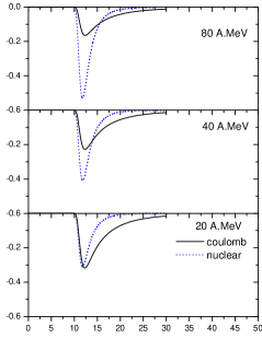
Figure 1: Nuclear and Coulomb breakup potentials

Eqs.(2), (3) and (4) show that the imaginary part of the phase shift and the modulus square of the S-matrix which takes into account the breakup channel can be simply obtained from the breakup probability and it would not be necessary to know the actual form of the optical potential. However to understand the physical origin of its characteristics and in order to use elastic scattering data for structure studies it is useful to deduce an analytical form of it. To this goal we have followed the method outlined in Sec. 2.1. We started by calculating the total Coulomb and nuclear breakup probabilities from the numerical integration over the neutron final continuum energy of Eqs. (7) and (13). The neutron-target optical potential used here to calculate the neutron breakup probabilities is from Ref.[39] and it has the usual Woods-Saxon form for the real and imaginary volume parts and a Woods-Saxon derivative form for the surface imaginary part. The parameter values are given in Table 1. We then fitted the total probabilities to a sum of exponentials. This allows a simple extraction of the potential from the relation Eq.(11) and also a transparent physical interpretation of the large diffusness.

$$p^{N}(b_{c})=\sum_{n}A_{n}~{}\exp{(-b_{c}/\alpha_{n})},$$ (16)

$$p^{C}(b_{c})=\sum_{n}B_{n}~{}\exp{(-b_{c}/\beta_{n})},$$ (17)

Table 2: Best fit obtained for the nuclear and Coulomb halo breakup probabilities Eqs.(7),(13) for ¹¹Be incident on ²⁰⁸Pb. The parameters $\alpha_{n}$ and $\beta_{n}$ are in fm, while $A_{n}$ and $B_{n}$ are dimentionless. Incident energies in A.MeV

		Nuclear			Coulomb
$E_{inc}$	20	40	80	20	40	80
$A_{1}$	1860.38	303.23	339.45	9.672	3.922	1.734	$B_{1}$
$A_{2}$	19.73	7.91	1.91	1.558	0.6013	0.2549	$B_{2}$
-	-	-	-	0.1531	0.0587	0.0248	$B_{3}$
$\alpha_{1}$	1.1924	1.5334	1.5356	2.7273	2.9438	3.1046	$\beta_{1}$
$\alpha_{2}$	2.5403	2.7918	3.4955	6.5189	7.4850	8.2713	$\beta_{2}$
-	-	-	-	15.6863	19.9322	24.1546	$\beta_{3}$

The corresponding parameters are given in Table 2. The parameters $\alpha_{n}$ and $\beta_{n}$ obtained show clearly that the exponential tail of the breakup probabilities have a very long range, in particular in the Coulomb breakup case. To obtain forms of the potentials valid at all distances, we used then Eqs.(5), (10) and (11), renaming again $b_{c}$ with $r$ such that

$$W^{N}_{S}(r)=-{\hbar v\over 2}P_{0}\sum_{n}A_{n}~{}\exp{(-r/\alpha_{n})}{1\over\sqrt{2\pi\alpha_{n}r}}.$$ (18)

$$W^{C}_{S}(r)=-{\hbar v\over 2}P_{0}\sum_{n}B_{n}~{}\exp{(-r/\beta_{n})}{1\over\sqrt{2\pi\beta_{n}r}}.$$ (19)

The core survival probability has been parameterized as

$$P_{0}(b_{c})=|S_{CT}|^{2}=\exp(-\ln 2e^{[(R_{s}-b_{c})/a_{0}]}),$$ (20)

where $a_{0}=0.6fm$ and $R_{s}=1.4(A_{P}^{1/3}+A_{T}^{1/3})fm$ is the strong absorption radius [47].

3 Results

Table 3: Optical potential parameters for the bare ¹⁰Be, ¹¹Be-²⁰⁸Pb interaction. Radii are calculated with the $R_{i}=r_{i}(A_{P}^{1/3}+A_{T}^{1/3})$fm convention.

Energy(A.MeV)	V	$r_{V}$	$a_{V}$	Wv	$r_{W}$	$a_{W}$
20	-80	1.020	0.78	-66.7	1.110	0.39	[42]
40	-70	0.920	1.04	-58.9	0.890	0.89	[43]
80	-36	1.087	0.78	-40.0	1.040	0.41	[44]

In order to sample the quantitative accuracy of the simple analytical model presented above we discuss now some numerical examples. The potentials we will discuss derive from the breakup of the $2s_{1/2}$ state of ¹¹Be, with separation energies $0.5MeV$, asymptotic normalization constant $C_{i}=0.91fm^{-1/2}$ and spectroscopic factor $C^{2}S=0.77$. $C_{i}$ was obtained from a wave function calculated in a Woods-Saxon potential with radius parameter $r=1.25fm$, diffuseness $a=0.8fm$ and depth $V_{0}=-52.4MeV$, adjusted to fit the neutron separation energy.

\psfrag{sigmar\r{missing}}{$\sigma/\sigma_{R}$ }\psfrag{thetar\r{missing}}{$\theta$ ${}_{C.M}$ (deg)}\psfrag{this bare potential fixed for 40 mev/n for all.\r{missing}}{.}\includegraphics[scale={.35},angle={0}]{comparison33.eps}

\psfrag{sigmar\r{missing}}{$\sigma/\sigma_{R}$ }\psfrag{thetar\r{missing}}{$\theta$ ${}_{C.M}$ (deg)}\psfrag{this bare potential fixed for 40 mev/n for all.\r{missing}}{.}\psfrag{sigmar\r{missing}}{ .}\includegraphics[scale={.35},angle={0}]{comparison44new.eps}

Figure 2: Comparison between the results of two calculations according to the eikonal model (solid line) and the optical model (dotted line) at 20, 40 and 80 A.MeV for ¹⁰Be +²⁰⁸Pb with the potential [43], right hand figure, and with the potential [44], left hand figure.

As we discussed already in detail in Ref.[5] the diffuseness of the nuclear breakup potential is a very important parameter. It depends weakly on the incident energy and its large value between 2 and 3 fm is due to the large decay constant of the neutron halo wave function and thus to the low separation energy. In the case of the Coulomb potential we see that the diffuseness $\beta_{n}$ is even larger, and furthermore increasing with energy. This is clearly a reflection of the long range, energy dependent effects of the Coulomb potential itself and of the core-recoil it causes.

From the diffuseness parameters values shown in Table 2 we notice that at each incident energy the largest diffuseness values are

$$\beta_{3}\approx(\varepsilon_{k}^{max}-\varepsilon_{i})/\hbar v$$ (21)

where $\varepsilon_{k}^{max}=2\div 3MeV$ is of the order of the largest continuum energy for which there is an appreciable breakup probability. This effect is clearly related to the behavior at very large distances of the Bessel functions $K_{0,1}\approx e^{-\varpi}$ in Eq.(13). Therefore in the case of the Coulomb breakup potential the diffuseness value is related to the adiabaticity parameter and it depends on the initial separation energy but also, strongly, on the incident energy. Thus this potential is much more dependent from the reaction dynamics than the nuclear breakup potential.

\psfrag{sigmar\r{missing}}{$\sigma/\sigma_{R}$ }\psfrag{theta\r{missing}}{$\theta$ ${}_{C.M}$ (deg)}\includegraphics[scale={.45},angle={0}]{20total1.eps}

Figure 3: Angular distribution for the elastic scattering at 20 A.MeV of ¹⁰Be and ¹¹Be from ²⁰⁸Pb.

We show now in Fig.1 the radial shapes of the potentials calculated for the breakup from the $2s$ state of ${}^{11}Be$ in the interaction with ${}^{208}Pb$. Results are given for three laboratory incident energies: E_inc=20 A.MeV, 40 A.MeV and 80 A.MeV. The solid lines are the Coulomb breakup potentials while the dotted lines are the nuclear breakup potentials. As discussed above our results show that the potentials are energy dependent and the Coulomb breakup potential has a much longer range than the nuclear breakup potential.

\psfrag{sigmar\r{missing}}{$\sigma/\sigma_{R}$ }\psfrag{theta\r{missing}}{$\theta$ ${}_{C.M}$ (deg)}\includegraphics[scale={.35},angle={0}]{40total2.eps}

Figure 4: The same as Fig. 3 but at 40 A.MeV

The optical potential has one of its most interesting application in the calculation of elastic scattering angular distributions. Since according to Eqs.(2) and (10) our phase shifts for the breakup channels are calculated in the eikonal model, it seems appropriate to calculate the angular distributions within the same model. Therefore we first show in Fig. 2 a comparison of calculations made with the optical model code OPTIM [40] and with our modified version of the eikonal code DWEIKO [41] for the reaction at the same energies at which potentials have been given in Fig.1. For the lowest energy DWEIKO contains a further recoil correction obtained by shifting the integration impact parameter, as explained in Ref.[41]. The optical model parameters for the volume parts of the bare potential are given in Table 3. Since there are no data in the literature for the ¹⁰Be+²⁰⁸Pb system at the incident energies we are concerned with we have tried to use two modified potentials obtained from fits of ¹²C+²⁰⁸Pb [43] and ⁴He+²⁰⁸Pb [44] data. It is clear that for both potentials the eikonal model works very well up to 10^o. At very high incident energies when an optical model code could have difficulties in handling the large number of partial waves necessary for heavy ions, an eikonal calculation is much simpler and equally accurate. A serius problem for the check of accuracy of theoretical models and related numerical applications of the kind of problems discussed in this paper is the lack of experimental data and of reliable bare potentials for the core-target interaction. Therefore the calculations discussed in the following have to be considered as exploratory.

In Figs. 3, 4 and 5 we show then the eikonal model angular distributions for ¹⁰Be+²⁰⁸Pb by the thick solid line. The thin solid line is for ¹¹Be+²⁰⁸Pb with the bare volume potential of Table 3. The dashed and dotted lines include the Coulomb breakup and the nuclear breakup potentials respectively, while the dot-dashed line includes both. As expected in most of the angular range the Coulomb breakup reduces the elastic scattering more than the nuclear breakup.

\psfrag{sigmar\r{missing}}{$\sigma/\sigma_{R}$ }\psfrag{theta\r{missing}}{$\theta$ ${}_{C.M}$ (deg)}\includegraphics[scale={.35},angle={0}]{80total1.eps}

Figure 5: The same as Figs. 3 and 4 but at 80 A.MeV

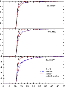
Figure 6: Scattering matrix with and without breakup potentials contributions

Finally we discuss another important effect namely how the elastic scattering total probability changes as a function of the impact parameter or angular momentum when there is a large breakup. In Fig.6 we show with the solid line the core-target S-matrix $S_{CT}$. Because of the incertitudes in the bare optical potentials used for the angular distribution calculations we prefer here to use for $S_{CT}$ a unique form given by Eq.(20). The nucleus-nucleus S-matrix $S_{NN}$, shown by the dot-dashed line, is calculated then from Eq.(4), which contains the effect of the halo breakup. At a fixed impact parameter the effect of the breakup is to reduce the elastic probability given by the modulus square of the S-matrix. The unitary limit is attained at much larger $b_{c}$-values and the reaction cross section receives significant contributions from a large range of impact parameters. The reduction is obviously more pronounced at the impact parameters larger than the strong absorption radius. The value of the strong absorption radius, defined as $|S_{NN}(R_{s})|^{2}={1\over 2}$ changes appreciably, increasing of about 1 fm at 20 A.MeV, 0.8 fm at 40 A.MeV and 0.6 fm at 80 A.MeV. The large increase is mainly due to the Coulomb breakup effect. This can be seen by looking at the dotted and dashed lines which represent $S_{NN}$ when only the nuclear or the Coulomb breakup effect is included, respectively.

Another significant effect of the imaginary surface potential is seen in the reaction cross sections obtained from the $S_{NN}$ and given in Table 4. We show also a number of other cross section values necessary to justify the phenomenological inputs of our calculations and their consistency. The first two rows give the total cross sections for the systems ¹⁰Be + ²⁰⁸Pb and ¹¹Be + ²⁰⁸Pb respectively, calculated with the bare optical potentials of Table 3. The cross sections in the next three rows contain also the effect of the nuclear breakup, of the Coulomb breakup and of both at the same time. All these cross sections have been calculated in the eikonal approximation with the code DWEIKO. There is an increase of the order of 500$\div$600 mb with respect to the bare (no breakup) optical potential when the nuclear breakup potential is taken into account. When the Coulomb breakup is included we find an increase of about 1.6 b to 4.4 b depending on the incident energy. The total increase in the reaction cross section is very large, corresponding to a variation of a factor from 2 to 3 at some energies. Similar increases in the cross sections have been found in Ref.[15]. These values are consistent with the nuclear and Coulomb breakup cross sections obtained from the integration over the core-target impact parameter of the probabilities Eqs.(7) and (13) including the core survival probability Eq.(20) and given in the next two rows. Finally the free particle n-Pb elastic, inelastic and total cross sections obtained in the eikonal model by using the potentials of Table 1 are given. The last row contains the experimental free particle cross sections. As expected at 20MeV our free particle cross sections are still not very close to the experimental values, but already at 40MeV the eikonal approximation works very well.

As discussed already in [5], the relation between the total reaction cross section and the breakup cross section, can be understood by expanding the exponential in Eq.(4) to first order in $P_{b_{up}}$ and integrating over the impact parameter $b_{c}$. One immediately finds

$$1-|S_{NN}(b_{c})|^{2} \approx 1-|S_{CT}(b_{c})|^{2}e^{-P_{b_{up}}(b_{c})}$$ (22)

$$= 1-|S_{CT}(b_{c})|^{2}+$$

$$+|S_{CT}(b_{c})|^{2}(p^{N}_{b_{up}}(b_{c})+p^{C}_{b_{up}}(b_{c}))$$

$$\sigma_{NN} = 2\pi\int b_{c}db_{c}\left(1-|S_{NN}(b_{c})|^{2}\right)$$ (23)

$$\approx \sigma_{CT}+\sigma^{N}_{b_{up}}+\sigma^{C}_{b_{up}}.$$ (24)

The fact that the cross sections values of Table 4 are in very good agreement with the relations contained in Eqs.(23) and (24) is a proof of the accuracy of the hypothesis Eq.(4) for the nucleus-nucleus S-matrix and of the separation of the imaginary potential into a volume and a surface term, with the surface term identified with the halo breakup potential.

Table 4: Cross section values (in mb) discussed in this paper. See text for details.

	Energy(A.MeV)	20	40	80
${}^{10}Be+^{208}Pb$ total cross section	$\sigma_{CN}$	2362	2897	2537
${}^{11}Be+^{208}Pb$ total cross section with bare potential	$\sigma_{NN}$	2644	2969	2593
$\sigma_{NN}$ including nuclear breakup	$\sigma^{N}_{NN}$	3185	3471	3060
$\sigma_{NN}$ including coulomb breakup	$\sigma^{C}_{NN}$	6685	5477	4152
$\sigma_{NN}$ including coulomb and nuclear breakup	$\sigma^{N+C}_{NN}$	7074	5900	4584
nuclear halo breakup	$\sigma^{N}_{b_{up}}$	615	551	490
Coulomb halo breakup	$\sigma^{C}_{b_{up}}$	4280	2638	1570
n-${}^{208}Pb$ elastic free particle	$\sigma^{el}$	2554	2623	2467
n-${}^{208}Pb$ inelastic free particle	$\sigma^{in}$	2018	1902	2097
n-${}^{208}Pb$ total free particle	$\sigma^{Tot}$	4548	4437	4867
n-${}^{208}Pb$ experimental	$\sigma_{exp}$ [45]	5888	4392	4817

4 Conclusions

In conclusion we have presented a simple analytical method to obtain the surface component of the imaginary part of the nucleus-nucleus optical potential to be used in the elastic scattering calculations between a halo or weakly bound nucleus and a heavy target. The surface potential is due to Coulomb and nuclear breakup. The main purpose here was to relate the characteristics of the potential to the special properties of the breakup channels for weakly bound nuclei. At high incident energy ($>$ 20A.MeV) the evaluation of the potentials amounts in fact just to the calculation of the breakup probability as already shown in Ref.[5]. If breakup from core excited states is to be included, then it suffices to sum up the relative probabilities according to Eq.(3).

The method to include Coulomb breakup is an extension of that previously used to calculate microscopically the effect of transfer and nuclear breakup channels on the imaginary potential. The shape of the surface imaginary potential and its parameters are determined univocally by the shape of the breakup probability. An interesting result is that the diffuseness of the potential for the nuclear breakup reflects the decay length of the valence neutron wave function and therefore it depends mainly upon the projectile structure, but not so much on the reaction dynamics. For the Coulomb breakup there is instead a strong dependence on the dynamics which leads to an increase of the diffuseness value when increasing the incident energy. The strength is also energy dependent. Analytical calculations contained in appendix A have shown that the potential proposed here is consistent with and can be viewed as an extension to high energy, of other theoretical models developed at energies close to the Coulomb barrier [14]. The numerical calculations on the other hand show consistency with the works of other authors [15] for similar, light halo systems. Furthermore we have given an explicit justification for the long range of the polarization potential.

From Feshbach [50] formalism it is known that related to the imaginary potential, which comes from the second order, complex term, there is also a real correction to be added to the first order term, the folding potential. However it has been shown by the authors of Ref.[14] that the Coulomb excitation polarization potential is purely imaginary at high energy. On the other hand for the nuclear breakup potential, we have shown in Ref.[5] that the second order real correction is small and negligible, while other calculations [9, 12] for ${}^{11}Li$ projectile found a not so small real polarization potential. To make sure that the second order real correction is negligible also for heavy targets such as ²⁰⁸Pb, we have added phenomenologically a real repulsive part to our microscopically calculated imaginary potential, with the same exponential form, same diffuseness and variable strength, but we found no noticeable differences in the angular distributions. Two open questions remain then to be addressed for future work. One is which observable will be more sensitive to the real correction term. The other is a systematic microscopic calculation of such a term for a number of different systems and energies.

Acknowledgments

We are very grateful to Carlos Bertulani for providing and helping us using his code DWEIKO and for his very useful remarks on our manuscript. We wish to thank also David Brink and Alvaro Garcia-Camacho for discussions and Stefan Typel for providing us the good parameters of his potential. One of us (A.A.I) is very grateful to the Italian Ministry of Foreign Affairs for a one year grant under the scheme ’ Inter-University Cooperation. Scholarships and Youth Exchange Programmes’.

Appendix A Connection to low energy approaches

In our formalism the imaginary part of the optical potential due to Coulomb breakup is given by

$$\int_{-\infty}^{+\infty}W_{S}({\bf r}(t))dt=-{\hbar\over 2}p^{C}_{b_{up}},$$ (25)

while Eq. (12) of Andrés et al. [14] reads

$$\int_{-\infty}^{+\infty}W_{S}({\bf r}(t))dt=\hbar\alpha.$$ (26)

Where both $p^{C}_{b_{up}}$ and $\alpha$ depend on the incident energy and on the classical trajectory of relative motion. In our case such a trajectory is a straight line since our approach applies to incident energies well above the Coulomb barrier.

The two approaches are consistent if $\alpha\to-{p^{C}_{b_{up}}/2}$ in the high energy limit. To show that this is true we write explicitly the expression in Ref. [14]

$$\alpha=-{\pi\over 9}\left({Z_{T}e\over\hbar va_{c}}\right)^{2}\int d\varepsilon_{k}\left(I^{2}_{11}(\varpi)+I^{2}_{1-1}(\varpi)\right){dB(E1,\varepsilon_{k})\over d\varepsilon_{k}}$$ (27)

where $I_{1\pm 1}$ are the well known Coulomb integrals [46] which can be expressed in terms of Bessel functions of imaginary order. However according to Eq.(28) of Ref.[48] in the high energy limit

$$I(E1,\pm 1)=I_{1\pm 1}={2a_{c}\over b_{c}}\varpi K_{1}(\varpi),$$ (28)

where $a_{c}$ is the Coulomb length parameter and now $K_{1}$ is an ordinary Bessel function of real index.

On the other hand considering Eq.(15) for $p^{C}_{b_{up}}$ we remark that it is well known and shown for example in Fig.1 of Ref.[49] that $\varpi^{2}K_{0}^{2}\left(\varpi\right)$ is much smaller than $\varpi^{2}K_{1}^{2}\left(\varpi\right)$ for values of $\varpi\approx 0.1$, which happens for heavy ions at high energies. We can then write Eq.(15) as

$$p^{C}_{b_{up}}(b_{c})\approx{2\pi\over 9}\left({Z_{T}e\over\hbar vb_{c}}\right)^{2}\int d\varepsilon_{k}2\left(2\varpi K_{1}\left(\varpi\right)\right)^{2}{dB(E1,\varepsilon_{k})\over d\varepsilon_{k}}.$$ (29)

since for the case studied in this paper the explicit form of B(E1) is

$${dB(E1,\varepsilon_{k})\over d\varepsilon_{k}}=C^{2}S{\frac{m_{n}}{\hbar^{2}k}}(C_{i}{\beta}_{1}Z_{P}e)^{2}{6\over\pi^{2}}{k^{4}\over(k^{2}+\gamma^{2})^{4}},$$ (30)

which is the consistent with Eq.(6.5) of Ref.[49] or Eq. (7.24) of [28] and it is the explicit form of the B(E1) obtained for an s-initial state using the asymptotic form of the wave function.

Finally using Eq.(28) in Eq.(27) and comparing with Eq.(29) we obtain that $\alpha=-{p^{C}_{b_{up}}/2}$ in the high energy, straight line trajectory limit. However we remark that our probability Eq.(13) is more accurate than the high energy limit of $\alpha$ of Eq.(27) since it contains also the term representing longitudinal excitations, proportional to $K_{0}$ and to $k_{z}$, the parallel component of neutron momentum.

References

- [1] I. Tanihata et al., Phys. Lett. B 160 (1985) 380.
- [2] J. J. Kolata et al., Phys. Rev. Lett. 69 (1992) 2631. M. Lewitowicz et al., Nucl. Phys. A 562 (1993) 301. W. Mittig and P. Roussel-Chomaz, Nucl. Phys. A 693 (2001) 495 and references therein.
- [3] P. G. Hansen, A. S. Jensen, and B. Jonson, Ann. Rev. Nucl. Part. Sci. 45 (1995) 591 , and references therein.
- [4] F. Cappuzzello et al., Phys. Lett. B 516 (2001) 21 and private communication.
- [5] A. Bonaccorso and F. Carstoiu, Nucl. Phys. A 706 (2002) 322.
- [6] J. C. Pacheco and N. Vinh Mau, Nucl. Phys. A 669 (2000) 135.
- [7] N. Takigawa et al., Phys. Lett. B 288 (1992) 244.
- [8] Y. Sakuragi, S. Funada, Y. Hirabayashi, Nucl. Phys. A 588 (1995) 65c.
- [9] K. Yabana, Y. Ogawa and Y. Suzuki, Nucl. Phys. A 539 (1992) 295 . Phys. Rev. C 45 (1992) 2909.
- [10] L. F. Canto, R. Donangelo, M. S. Hussein and M. P. Pato, Nucl. Phys. A 542 (1992) 131. F. Canto, R. Donangelo, M. S. Hussein, Nucl. Phys. A 529 (1991) 243.
- [11] R. C. Johnson, J. S. Al-Khalili and J. A. Tostevin, Phys. Rev. Lett. 79 (1997) 2771.
- [12] J. S. Al-Khalili, J. A. Tostevin and J. M. Brooke, Phys. Rev. C 55 (1997) R1018.
- [13] J. S. Al-Khalili, Nucl. Phys. A 581 (1995) 315.
- [14] M.V. Andrés, J. Gómez-Camacho and M. A. Nagarajan, Nucl. Phys. A 579 (1994) 273.
- [15] R. S. Mackintosh and N. Keeley, Phys. Rev. C 70 (2004) 024604 and references therein.
- [16] M. S. Hussein and G. R. Satchler, Nucl. Phys. A 567 (1994) 165 .
- [17] D. T. Khoa, G. R. Satchler and W. von Oertzen, Phys. Lett. B 358 (1995) 14.
- [18] R. A. Broglia, and A. Winther, , Benjamin, Reading, Mass, 1981.
- [19] R. A. Broglia, G. Pollarolo and A. Winther, Nucl. Phys. A 361 (1981) 307.
- [20] A. Bonaccorso, G. Piccolo, D. M. Brink, Nucl. Phys. A441 (1985) 555.
- [21] Fl. Stancu and D. M. Brink, Phys. Rev. C 25 (1981) 2450. Fl. Stancu and D. M. Brink, Phys. Rev. C 32 (1985) 1937.
- [22] A. Bonaccorso and D. M. Brink, Phys. Rev. C 38 (1988) 1776.
- [23] A. Bonaccorso and D. M. Brink, Phys. Rev. C 43 (1991) 299.
- [24] A. Bonaccorso and D. M. Brink, Phys. Rev. C 44 (1991) 1559.
- [25] A. Bonaccorso and D. M. Brink, Phys. Rev. C 46 (1992) 700.
- [26] A. Bonaccorso and D. M. Brink, Phys. Rev. C 58 (1998) 2864.
- [27] C. A. Bertulani and P. Danielewicz, Nucl. Phys. A 717 (2003) 199.
- [28] C. A. Bertulani, M. S. Hussein, G. Münzenberg, Physics of Radioactive Beams, Nova Science Publishers, Inc., New York 2001.
- [29] A. Bonaccorso, D. M. Brink, C. A. Bertulani, Phys. Rev. C 69 (2004) 024615.
- [30] G. Baur, K. Hencken and D. Trautmann, Prog. Part. Nucl. Phys. 51 (2003) 487.
- [31] N. Fukuda et al., nucl-ex/0409020, to be published on Phys. Rev. C.
- [32] L. I. Schiff, Quantum Mechanics, Mc Graw-Hill Kogasha Ltd , Tokyo 1968, Pag. 130.
- [33] J. Margueron, A. Bonaccorso and D. M. Brink, Nucl. Phys. A 703 (2002) 105.
- [34] J. Margueron, A. Bonaccorso and D. M. Brink, Nucl. Phys. A 720 (2003) 337, Nucl. Phys. A 741 (2004) 381.
- [35] A. Bonaccorso and D. M. Brink, Nucl. Phys. A 384 (1982) 161.
- [36] A. Bonaccorso and G. F. Bertsch, Phys. Rev. C 63 (2001) 044604.
- [37] H. Esbensen and G. F. Bertsch, Phys. Rev. C 59 (1999) 3240 .
- [38] F. Canto, R. Donangelo, P. Lotti and M. S. Hussein, Nucl. Phys. A 589 (1995) 117.
- [39] C. Mahaux and R. Sartor, Adv. Nucl. Phys. 20 (1991) 1.
- [40] N. M. Clarke, 1994 (unpublished).
- [41] C. A. Bertulani, C. M. Campbell and T. Glasmacher, Comput. Phys. Commun. 152 (2003) 317 and private communication. In the published version of DWEIKO there is a typing mistake. A term -1 in the exponent of the imaginary part of the Woods-Saxon potential which was not expected to be there and we have corrected.
- [42] M. Buenerd et al., Nucl. Phys. A 424 (1984) 313.
- [43] S. Typel and R. Shyam, Phys. Rev. C 64 (2001) 024605 and private communication. There is a typing mistake in the radii of the core-target potentials printed in this paper.
- [44] M. Buenerd et al., Phys. Lett. B 102 (1981) 242.
- [45] R.W. Finlay et al., Phys.Rev. C 47 (1993) 237.
- [46] K. Alder and A. Winther, Electromagnetic Excitation, (North-Holland, Amsterdam, 1975).
- [47] D. M. Brink, Semiclassical methods for nucleus-nucleus scattering, Cambridge University Press. Cambridge. 1985.
- [48] C. A. Bertulani et al., Phys. Rev. C 68 (2003) 044609.
- [49] H. Esbensen, Proceedings of the 4th course of the International School in Heavy Ion Physics, 4th course, Erice, May 1997, Ed. R. A. Broglia end P. G. Hansen, World Scientific 1998.
- [50] H. Feshbach, Ann. Rev. Nucl. Sci. 8 (1958) 49.