Solutions of the Bohr hamiltonian, a compendium

Abstract

The Bohr hamiltonian, also called collective hamiltonian, is one of the cornerstone of nuclear physics and a wealth of solutions (analytic or approximated) of the associated eigenvalue equation have been proposed over more than half a century (confining ourselves to the quadrupole degree of freedom). Each particular solution is associated with a peculiar form for the $V(\beta,\gamma)$ potential. The large number and the different details of the mathematical derivation of these solutions, as well as their increased and renewed importance for nuclear structure and spectroscopy, demand a thorough discussion. It is the aim of the present monograph to present in detail all the known solutions in $\gamma-$unstable and $\gamma-$stable cases, in a taxonomic and didactical way. In pursuing this task we especially stressed the mathematical side leaving the discussion of the physics to already published comprehensive material.

The paper contains also a new approximate solution for the linear potential, and a new solution for prolate and oblate soft axial rotors, as well as some new formulae and comments, and an appendix on the analysis of a few interesting numerical sequences appearing in this context. The quasi-dynamical SO(2) symmetry is proposed in connection with the labeling of bands in triaxial nuclei.

PREPRINT - PRELIMINARY -

I Introduction

More than half a century has elapsed from the publication of one of the milestones of nuclear physics “The coupling of nuclear surface oscillations to the motion of individual nucleons” Bohr1 on the danish journal “Matematisk-fysiske Meddelelser” by Aage Bohr in 1952. The cited work contains the foundations of the collective model, developed fully in a second important work in collaboration with Ben R. Mottelson Bohr2 , and especially contains the first derivation of the subject of this monograph: the Bohr hamiltonian, also called collective hamiltonian or , sometimes, Bohr-Mottelson hamiltonian($H_{B}$). This operator contains kinetic as well as restoring potential terms in some set of variables describing the extent of deformation of the nuclear surface. The present paper, far from being a comprehensive review (that are numerous in the specialized literature Rev ; EG ) of the many physical topics, successes and applications of the collective model, is rather meant to provide the reader with an enumeration and mathematical discussion of the analytic and approximate solutions of the stationary eigenvalue equation $H_{B}\Psi=E\Psi$ with various form of the potentials and referring to different physical situations. Other developments originated from the collective model (as the Frankfurt model, the Baranger-Kumar model or the symplectic model) will not be discussed here.

The need for such a taxonomic compendium is, to our view, justified by the recent proliferation of new solutions that makes this topics exciting and, at the same time, significantly extended. The new solutions have received a considerable attention, both from theoreticians and from experimentalists, and application of these ideas or survey of spectroscopic data are constituting a very important research line. It is also our belief that these studies have reached a considerable degree of completeness and that a classification of the subject is therefore timely. To corroborate our views upon the renewed role of the collective model as a driving force for new research, we mention that an interesting paper, that contains some sections dedicated to the Bohr hamiltonian, has recently been published Jolos (See section V.6).

The problem of the solution of the Bohr hamiltonian has been mainly tackled in two ways: direct solution of the second order differential equation and use of algebraic techniques to exploit dynamical symmetries. The latter approach has also been used as a source of ’labels’ for various solutions of distinctive importance. A novel interest has been raised by the possibility to give analytical solution at the critical point of a shape phase transitions between various types of quadrupole deformed nuclear surfaces Iac1 ; Iac2 . Another method that is worth mentioning by virtue of the insight that one may get is the numerical diagonalization of the problem for complicated potentials that cannot be treated analytically. We will also remark on some of these cases.

After a brief discussion on the historical and scientific foundations of the collective model (Section II), we will be concerned with an analysis of the known solutions of the eigenvalue equation for the Bohr hamiltonian for $\gamma-$unstable (Section III), axial $\gamma-$stable (Section IV) and triaxial $\gamma-$stable (Section V) cases, with direct solution of the differential equation, which we will lay before the reader following, as far as possible, the course of time. Some comments on group theoretical techniques and solutions are also given (Section VI). Section VII contains a brief description of a few important recent advances that are connected with the main theme of this compendium.

Writing in a single paper a summary of works and efforts that have been devoted to the study of collective models and paying the tribute to every researcher involved in the matter would be a formidable task, and we have decided to confine ourselves to the work plan cited above, apologizing for any unintentional omission. We decided to label the solutions on the basis of their proposers, mainly to avoid confusion with the corresponding problems in the solution of the Schrödinger equation in the configuration space. Where the authors were many we used alternative titles.

This paper is not only a review, but contains some novelties as the treatment of the linear potential in Section III.H, that to our knowledge has never been treated in this context, or, for instance, formula (40). Moreover we propose a new solution for prolate and oblate soft axial rotors (Section IV.5) obtaining interesting patterns for $\gamma$ and $\beta$ excitations.
A critical discussion of the various cases is supplemented by few comments that may share light on specific points (as for instance in section 67). In the appendix we discuss from a purely number theoretical perspective, the problem of repetitions of quantum numbers, that, as far as we know, has never been discussed elsewhere: we give two new sequences and we evidence some curious connections with other fields.

II Foundations of the Collective Model

Niels Bohr, father of Aage Bohr and of the atomic theory, is among the proposers of the theory of nuclear surface oscillations Niels . The idea was to treat the nucleus as a liquid droplet, and that the fundamental collective modes of motion of the surface were linked to nuclear excitations. Let us quote Aage Bohr’s words Bohr1 about the liquid drop theory:

According to the liquid drop model, the fundamental modes of nuclear excitation correspond to collective types of motion, such as surface oscillations and elastic vibrations. Even if it has not been possible, with certainty, to associate observed nuclear levels with particular modes of oscillation, the model gives an immediate explanation of the rapid increase of level density with increasing excitation of the nucleus.

The fifty years elapsed since the time of the exposure of his ideas have contradicted the last sentence: it is indeed possible to associate solutions of the Bohr hamiltonian with nuclear spectra, giving an immediate explanation of many nuclear properties. The collective model, that was subsequently developed in collaboration with Ben R. Mottelson and that has taken the name of Bohr-Mottelson model, should be regarded, as Bohr was warning, as a complementary approach to the shell model and should shed light only on some aspects of the still dim complexity of nuclear spectra.

The innovative idea underlying the already cited work was

…to consider various properties of a nucleus described in terms of a deformable surface coupled to the motion of individual nucleons. This combined model may be referred to as the quasi-molecular model.

It is strange that the name proposed by the author has been lost. He found that his model bore a resemblance to the theory of molecules in the very same way in which the single particle shell model bore a resemblance to the atomic theory.

Bohr’s paper was confined to the treatment of a single nucleon interacting with the nuclear surface. The radius of the latter was expressed, in polar coordinates, as an expansion in spherical harmonics:

$$R(\theta,\phi)~{}=~{}R_{0}\Bigl{(}1+\sum_{\lambda,\mu}\alpha_{\lambda,\mu}Y_{\lambda,\mu}(\theta,\phi)\Bigr{)}\,,$$ (1)

where $R_{0}$ is the radius of the nucleus when it has the spherical equilibrium shape. The expansion parameters $\alpha_{\lambda,\mu}$ are the coordinates that define a multidimensional space, whose points represent a deformed surface. The requirement of reality for the nuclear radius implies

$$\alpha_{\lambda,\mu}~{}=~{}(-1)^{\mu}\alpha_{\lambda,-\mu}^{*}\,.$$ (2)

The consistency of expansion (1) with the ’atomicity’ of the nucleus, i.e. the fact that it is composed by smaller particles, the nucleons, is assured by realizing that the idea of a continuous surface loses its meaning if one takes into consideration surface elements whose dimensions are comparable with the average distances between the constituents. This happens whenever $\lambda$ is larger or equal to the linear dimensions of the nucleus, $A^{1/3}$.
In the following we will confine to the quadrupole degree of freedom ($\lambda=2$) leaving aside the discussions about other multipolarities: in fact quadrupole states are the most fundamental collective type of low-lying excitations in nuclei and deserve a thorough analysis. If only small values of $\alpha$’s are taken into account the quadrupole deformed surface is an ellipsoid randomly oriented in space. The five coordinates $\{\alpha_{2,\mu}\}$ may thus be mapped onto a set of other five variables $\{a_{0},a_{2},\theta_{1},\theta_{2},\theta_{3}\}$, three of which describe angular orientations of the ellipsoid, the other two parameters being related to the extent of the deformation. This mapping from the frame of reference $R$ to a second frame of reference $R^{\prime}$, called ’intrinsic’, may be achieved via a unitary transformation:

$$a_{2,\nu} ~{}=~{} \sum_{\mu=-2}^{2}\alpha_{2,\mu}{\cal D}_{\mu,\nu}(\theta_{i})$$ (3)

$$\alpha_{2,\mu} ~{}=~{} \sum_{\mu=-2}^{2}a_{2,\nu}{\cal D}_{\mu,\nu}^{*}(\theta_{i})\,,$$ (4)

where ${\cal D}_{\mu,\nu}(\theta_{i})$ are the Wigner rotation functions for spherical harmonics with $\lambda~{}=~{}2$. The set of three angles $\{\theta_{i}\}$ describes the relative orientation of the two frames of reference. From now on we will drop the index $2$ since, as already said, we will deal only with quadrupole deformations. The transformation (4) may be conveniently chosen so that the axes of the frame of reference $R^{\prime}$ coincide with the principal axes of the ellipsoid. In this case

$$a_{1}=a_{-1}=0~{}~{}\mbox{~{}~{}~{}and~{}~{}~{}}~{}~{}a_{2}=a_{-2}\,.$$ (5)

The transformation of coordinates described above is however not unambiguous because of the possible different order of labeling of the axes and of the choice of the direction of the versors. This amounts to 48 sets of tranformed coordinates which correspond to the initial set (24 as long as right handed coordinate systems only are considered). The symmetry properties of the wave functions will be affected by the arbitrariness of the choice of the transformed coordinate system and this fact implies certain symmetry relations. Another substitution is required to reach a new set of coordinates $\{\beta,\gamma,\theta_{i}\}$ called the Hill-Wheeler coordinates, in which the subset $\{\beta,\gamma\}$ defines a two-dimensional polar coordinate system within the five-dimensional quadrupole deformation space, namely:

$$a_{0} ~{}=~{} \beta\cos{\gamma}$$ (6)

$$a_{2} ~{}=~{} (\beta/\sqrt{2})\sin{\gamma}\,,$$ (7)

with $\sum_{\mu}\mid\alpha_{\mu}\mid^{2}~{}=~{}\beta^{2}$. The total deformation of the nucleus is measured by $\beta$ in such a way that $\beta=0$ represents a sphere and $\beta\neq 0$ is an ellipsoid. The larger the value of $\beta$, the more deformed the surface. The parameter $\gamma$ describes the deviations from rotational symmetry: whenever $\gamma~{}=~{}n{\pi\over 3}$, with $n\in\mathbb{Z}$, two of the three semi-axes are of equal length. This is depicted in fig. 1.

Figure 1: Hill-Wheeler coordinates $\{\beta,\gamma\}$. The quadrupole deformed shapes corresponding to $\beta=0.4$ and $\gamma=n\pi/3$ (with $n=0,...,5$) are shown for reference. Different colors are connected with different principal axes of symmetry (green for z, red for y and blue for x).

To each (solid-line) radius in the polar plot of this figure corresponds an axially symmetric ellipsoid with a well-specified symmetry axis and a given character for what concerns prolateness or oblateness. Every point in the areas within the radii corresponds to triaxial shapes, that are characterized by three different semi-axes.

A convenient way to deal with quadrupole surfaces is to rewrite eq. (1) in terms of the new variables. The three radii defining the ellipsoid in the body-fixed frame are thus

$$R_{k}~{}=~{}R_{0}\Bigl{[}1+{5\over 4\pi}\beta\cos{\bigl{(}\gamma-{2\over 3}\pi k\bigr{)}}\Bigr{]}$$ (8)

with $k=1,2,3$ .

Now we are ready to introduce the Bohr hamiltonian, that is the hamiltonian built with generalized coordinates and momenta in quadrupole deformation space:

$$H_{B}~{}=~{}T+V~{}=~{}\sum_{\mu}\Bigl{\{}{1\over 2B_{2}}\mid\pi_{\mu}\mid^{2}+{C_{2}\over 2}\mid\alpha_{\mu}\mid^{2}\Bigr{\}}$$ (9)

where $B_{2}$ (that will be called $B_{m}$ i n the following) and $C_{2}$ are the mass and stiffness parameters of the liquid drop model for the quadrupole multipolarity. Here $\pi_{\mu}$ are the conjugate momenta associated to $\alpha_{\mu}$. We wish to call ’Bohr hamiltonian’ the set of more general expressions in which the potential term is a generic function of the parameters. We separate the Bohr hamiltonian into three terms:

$$H_{B}~{}=~{}T_{vib}+T_{rot}+V.$$ (10)

All the above terms are in general functions of $\beta$ and $\gamma$. The first term is the kinetic energy term related with shape vibrations with fixed orientation in space, the second instead is the kinetic energy of a rotational motion of the nuclear surface without any change of shape. The third term is the restoring potential in the shape parameters. Without entering into the details of the derivation Jean we merely restate the definitions of the two kinetic terms using the ${\beta,\gamma}$ variables:

$$T_{vib} = -{\hbar^{2}\over 2B_{m}}\Biggl{\{}{1\over\beta^{4}}{\partial\over\partial\beta}\beta^{4}{\partial\over\partial\beta}+{1\over\beta^{2}}{1\over\sin{3\gamma}}{\partial\over\partial\gamma}\sin{3\gamma}{\partial\over\partial\gamma}\Biggr{\}}$$

$$T_{rot} = {\hbar^{2}\over 2B_{m}}{1\over 4\beta^{2}}\sum_{k=1}^{3}{Q_{k}^{2}\over\Bigl{[}\sin{(\gamma-{2\pi\over 3}k)}\Bigr{]}^{2}}\,.$$ (12)

The vibrational part is usually divided into a $\beta$ and a $\gamma$ part (corresponding to the two terms in parenthesis in (LABEL:tvib)), though the two variables are actually mixed by the second term. We will consider potential energies that are only function of the internal coordinates $\beta$ and $\gamma$. The wave functions $\Psi(\beta,\gamma,\theta_{i})$ are solutions of the eigenvalue equation $H_{B}\Psi~{}=~{}E\Psi$ for the hamiltonian (10).

It may be thought that, in some sense essentially, the equation to solve is nothing but the Schödinger equation and that the record of cases that have already been known in the quantum mechanical context, apply to the present situation as well. This is partly true, but there are anyway a number of major differences that must be underlined and for which the collective hamiltonian deserves special cares: the Bohr equation is richer being expressed in terms of two variables (read two out of five), its ’natural’ space is five dimensional instead of three dimensional and these affects not only asymptotic behaviours and boundary conditions (that would be trivial), but also the group structure that we can identify with the Bohr hamiltonian.

The main part of the following will be concerned with $\gamma-$unstable solution, that is to say, exact solutions with a potential that is independent of $\gamma$. At the end of this enumeration we will treat approximate solutions with potentials that have also some dependence on $\gamma$.

III $\gamma-$unstable cases

Whenever the potential energy is only a function of $\beta$ the hamiltonian is separable Wilet . Setting

$$\Psi(\beta,\gamma,\theta_{i})~{}=~{}f(\beta)\Phi(\gamma,\theta_{i})$$ (13)

we may write two equations, one for the $\beta$ variable,

$$\Biggl{\{}{\hbar^{2}\over 2B_{m}}\Bigl{(}-{1\over\beta^{4}}{\partial\over\partial\beta}\beta^{4}{\partial\over\partial\beta}+{\Lambda^{2}\over\beta^{2}}\Bigr{)}+V(\beta)\Biggr{\}}f(\beta)~{}=~{}Ef(\beta)$$ (14)

that may alternatively be expressed in the canonical form as

$$\Biggl{\{}{\hbar^{2}\over 2B_{m}}\Bigl{(}-{\partial^{2}\over\partial\beta^{2}}+{(\tau+1)(\tau+2)\over\beta^{2}}\Bigr{)}+V(\beta)\Biggr{\}}(\beta^{2}f(\beta))~{}=~{}E(\beta^{2}f(\beta))$$ (15)

and the other for the $\gamma$ variable

$$\Biggl{\{}-{1\over\sin{3\gamma}}{\partial\over\partial\gamma}\sin{3\gamma}{\partial\over\partial\gamma}+{1\over 4}\sum_{k=1}^{3}{{\hat{Q}}^{2}_{k}\over(\sin{(\gamma-{2\pi\over 3}k)})^{2}}\Biggr{\}}\Phi(\gamma,\theta_{i})=\Lambda\Phi(\gamma,\theta_{i})\,,$$ (16)

where $\Lambda~{}=~{}\tau(\tau+3)$ is the separation parameter with $\tau~{}=~{}0,1,2,...$ . Since the potential is only a function of $\beta$, the angular momentum ${\hat{\bf Q}}^{2}$ and its third component ${\hat{Q}}_{z}$ are constants of motion and the quantum numbers associated with them, $L$ and $M$, are thus good quantum numbers. The so-called $\gamma-$angular part of the wavefunction may be written as

$$\Phi(\gamma,\theta_{i})~{}=~{}\sum_{K=-L}^{L}g_{K}^{L,\tau,\nu}{\cal D}_{M,K}^{L}(\theta_{i})\,,$$ (17)

where the rotation functions are eigenfunctions of the two operators ${\hat{Q}}_{z}$ and ${\hat{Q}}_{3}$, respectively the third component of the angular momentum vector along the z axis in the fixed frame of reference (eigenvalue M) and the third component of the angular momentum vector along the z’ axis in the intrinsic frame of reference of the nucleus (eigenvalue K). The functions $g$, that have the property $g_{K}~{}=~{}g_{-K}$, are given explicitely by Bés Bes and in addition to $L$ and $M$, are also labeled by other two quantum numbers $\tau$ and $\nu$. The former is the quantum number that comes from the solution of the eigenvalue equation of the Casimir operator of the SO(5) group (also called SO(5) seniority), while the latter is an empirical label needed in order to distinguish between the occurrence of multiple set of the same $L,M$ within a given SO(5) IR and takes the values Corr :

$$\nu~{}=~{}0,1,2,~{}...~{},[\tau/3]\,,$$ (18)

where square brackets indicates the integer part. Here we cannot omit to underline a fact that is worthy of remark: Bohr correctly denoted with $\tau$ the set of these two quantum numbers, but sometimes in the literature the $\tau$ quantum number has been taken as the label of SO(5) (as we do) and the $\nu$ quantum number has been left out (or forgot!). We think that the reason of this omission is that the importance of $\nu$ is seen only when one takes into account states with $\tau\geq 6$. In appendix A we give a detailed discussion of the determination of the sequence of repetitions.
The $K$ quantum number takes the value $\tau-3\nu$ and for each $K$ one has the following list of possible $L$’s:

$$L=2K,2K-2,2K-3,\cdots,K$$ (19)

that is to say all the integers between $K$ and $2K$ except for $2K-1$. The resulting spectrum displays a typical degeneracy pattern in energy that is summarized in table I.

$\tau$	$\nu$	$K$	$L$
0	0	0	0
1	0	1	2
2	0	2	2,4
3	0	3	3,4,6
	1	0	0
4	0	4	4,5,6,8
	1	1	2
5	0	5	5,6,7,8,10
	1	2	2,4
6	0	6	6,7,8,9,10,12
	1	3	3,4,6
	2	0	0

Table 1: Quantum numbers for the $\gamma-$unstable states. Every group of states with the same $\tau$ has the same energy. The lowest possible multiple occurrence of states with the same $L$ within a given IR of SO(5) is marked in red (See appendix for details).

The sets of quantum numbers and the $\Phi$ eigenfunctions of (16) discussed above are common to all $\gamma-$unstable problems of this section. The main differences in the spectra are thus to be searched in eq. (15), where in principle every possible potential function may be chosen. It is our aim to give here a discussion, as complete as possible, of the known cases.

III.1 Bohr’s harmonic oscillator solution

The solution given by A.Bohr Bohr1 was historically the first one. He put from the beginning an oscillator potential of the form

$$V(\beta)~{}=~{}{1\over 2}C\sum_{\mu=-2}^{2}\mid\alpha_{\mu}\mid^{2}~{}=~{}{1\over 2}C\beta^{2}$$ (20)

in eq. (15), obtaining the harmonic oscillator hamiltonian in a five dimensional space. The potential $V(\beta,\gamma)$ is depicted in fig. 2.

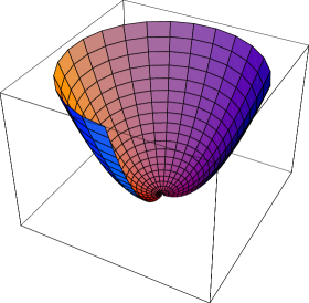
Figure 2: Plot $V(\beta,\gamma)$ of the harmonic oscillator potential (20) discussed by Bohr with $C=1$ and $0<\gamma<3\pi/2$.

The spectrum is given by

$$E=(N+5/2)\hbar\omega$$ (21)

with $\omega=\sqrt{C/B}$ and

$$N~{}=~{}\sum_{\mu}n_{\mu}~{}=~{}2n_{\beta}+\tau$$ (22)

with $N=0,1,2,3,...$ . The numbers $n_{\mu}$ represent the number of phonons with a given $\mu\hbar$ component of angular momentum along the z axis. The last relation evidences the fact that the $\gamma-$unstable case, with a harmonic oscillator spectrum and a minimum in $\beta=0$, has a further degeneracy with respect to the case discussed above: to a given $N$ may correspond different sets of $(n_{\beta},\tau)$.

$N$	$(n_{\beta},\tau)$	$L$
0	(0,0)	0
1	(0,1)	2
2	(0,2)	2,4
	(1,0)	0
3	(0,3)	0,3,4,6
	(1,1)	2
4	(0,4)	2,4,5,6,8
	(1,2)	2,4
	(2,0)	0

Table 2: Quantum numbers for the $\gamma-$unstable states of the harmonic oscillator potential. Every group of states with the same $N$ has the same energy. The first repetitions are marked in red. See appendix A and text for details on the sequence of repetitions.

With the content of Table I in mind, we list in Table II the quantum numbers of the first few states. States with the same $N$ have the same energy. We perform also in this case the analysis of the number of repetitions, that can be found in appendix A.

It is customary to normalize the energies in such a way that the lowest state is at 0, and the first excited is at 1. This normalization is equivalent to set the overall energy scale and the relative energy scale respectively. It turns out, obviously, that the energy of the second group of excited states in this energy scale is at 2. The ratio $R_{4/2}=E_{4^{+}}/E_{2^{+}}$, or better $(E_{4^{+}}-E_{0^{+}})/(E_{2^{+}}-E_{0^{+}})$, is the standard reference point for all the solutions of the collective hamiltonian and for the comparison with experimental data. Thus, for the harmonic oscillator, we have $E_{4^{+}}/E_{2^{+}}~{}=~{}2$. The indexes are referred to the labeling of the states from the bottom to the top. This is unambiguous for the present case, but in the following we will encounter many situations in which the degeneration typical of the harmonic oscillator will be removed and we will have two indexes, in order to distinguish between different bands (or families) of states and between different states within a given family.

It is useful to introduce the reduced energy $\epsilon=E{2B_{m}\over\hbar^{2}}$ and reduced potential $v(\beta)=V(\beta){2B_{m}\over\hbar^{2}}$ in eq. (15). In the case we are discussing $v(\beta)=k\beta^{2}$ with $k=CB/\hbar^{2}$ and hence

$$\Biggl{\{}-{1\over\beta^{4}}{\partial\over\partial\beta}\beta^{4}{\partial\over\partial\beta}-\epsilon+{(\tau+1)(\tau+2)\over\beta^{2}}+k\beta^{2}\Biggr{\}}f(\beta)~{}=~{}0$$ (23)

with normalized solution

$$f_{n}^{\tau}(\beta)=\Biggl{[}{2n!\over\Gamma(n+\tau+5/2)}\Biggr{]}^{1/2}\beta^{\tau}L_{n}^{\tau+3/2}(\beta^{2})e^{-\beta^{2}/2}$$ (24)

that contains associated Laguerre polynomials.

We display in fig. 3 the lowest energy states for the harmonic oscillator.

Figure 3: Spectrum of the harmonic oscillator potential. The energy scale ($\varepsilon^{\prime}$) is chosen by fixing $\hbar\omega=1$. See text and table II for explanations.

III.2 Wilets and Jean’s solutions

After a very clear and concise introduction to the subject, Wilets and Jean Wilet gave the solution in a couple of cases: the infinite square well and the displaced harmonic oscillator.

III.2.1 ’Anharmonic oscillator’

Their aim was to discuss the addition of anharmonicities to the $\beta$ potential and they took as a limiting case what they called, with a somewhat misleading designation, ’anharmonic oscillator’. In reality they were the first to treat the case of the infinite square well in the form

$$V(\beta)~{}=~{}\left\{\begin{array}[]{ccc}const&,&\beta<\beta_{w}\\ \infty&,&\beta>\beta_{w}\end{array}\right.$$ (25)

where $\beta_{w}$ takes a non-null positive real value. They gave the eigenenergies in terms of zeros of the Bessel functions and they found that the ratio $R_{4/2}$ is 2.20, but they said (cited work):

…, it represents the extreme case, not realizable in nature.

It seems thus that they underestimated the importance of this solution. In fact, only recently, Iachello Iac1 realized that this potential may furnish a good description for the shape phase transition between spherical and $\gamma-$unstable nuclei, although the real form of the potential at the critical point is, to the leading order, a quartic oscillator: the infinite square well approximates very well the behaviour of the $\beta^{4}$ potential, being very flat around the origin, and displays a qualitative agreement with the quickly rising asymptotic behaviour of the quartic potential at infinity. We will discuss later his solution, that provides not only the spectrum, but also eigenfunctions and transition rates. We will thus describe the complete solution for this potential as it is given in Iac1 , in the appropriate section.

III.2.2 Displaced harmonic oscillator

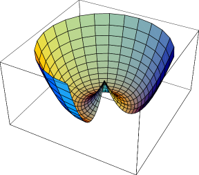
Figure 4: Plot $V(\beta,\gamma)$ of the displaced harmonic oscillator potential (26) discussed by Wilets and Jean with $C=2$ and $\beta_{0}=0.6$ (these values are chosen merely for purpose of illustration) and $0<\gamma<3\pi/2$.

The same authors treated the modification of the harmonic potential, called displaced harmonic potential, whose expression is given by

$$V(\beta)~{}=~{}{1\over 2}C(\beta-\beta_{0})^{2}.$$ (26)

It was introduced to describe a situation where the minimum along the $\beta$ direction is located at some fixed value $\beta_{0}$ (see fig. 4). With the substitutions:

$$x=\sqrt{B\omega\over\hbar\beta},\quad\epsilon={E\over\hbar\omega},\quad\varphi(x)=x^{2}f(\beta)$$

one can recast equation (15) in the following form

$${1\over 2}\Biggl{(}{\partial^{2}\over\partial x^{2}}-{(\tau+1)(\tau+2)\over x^{2}}-(x-x_{0})^{2}\Biggr{)}\varphi(x)=\epsilon\varphi(x)\,.$$ (27)

Wilets and Jean considered the potential formed by the displaced harmonic oscillator plus the $1/x^{2}$ term and expanded it in Taylor series around the minimum $x^{\prime}$ obtaining

$$v(x)\equiv{1\over 2}\Biggl{(}{(\tau+1)(\tau+2)\over x^{2}}+(x-x_{0})^{2}\Biggr{)}~{}=~{}v(x^{\prime})+{\omega^{\prime 2}\over 2}(x-x^{\prime})^{2}+O\bigl{(}(x-x^{\prime})^{3}\bigr{)}\,.$$ (28)

Neglecting terms of order three the effective potential is approximated by a harmonic oscillator and therefore the spectrum may be written as

$$\epsilon~{}=~{}(n_{\beta}+1/2)\omega^{\prime}+v(x^{\prime})\,,$$ (29)

with $n_{\beta}~{}=~{}0,1,2,...$. The spectrum looks like the one in fig. 3 with some proper scaling and shift of the energies. The eigenfunctions read

$$\varphi(x)~{}=~{}h_{n_{\beta}}\bigl{(}(x-x^{\prime})\sqrt{\omega^{\prime}}\bigr{)}e^{-(x-x^{\prime})^{2}\omega/2}\,,$$ (30)

where $h$ denotes Hermite polynomials. This is not an exact solution, but it is worth saying that it is a very good approximation for large values of $x_{0}$.

III.3 Elliott-Evans-Park’s solution for the Davidson potential.

Davidson Dav introduced a potential of the form $ar^{2}+b/r^{2}$ for the interaction between the constituents of a diatomic molecule. Elliott and collaborators Elli ; Elli2 employed (though they were not historically the firsts, see section on the Warsaw solution!) a similar form in the context of quadrupole deformations and Rowe and Bahri Rowe1 gave a detailed algebraic discussion of this potential both for molecular and nuclear spectra (see section VI).

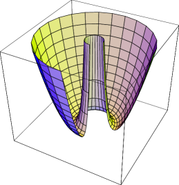
Figure 5: Plot $V(\beta,\gamma)$ of the Davidson potential (31) discussed analytically by Elliott et al. Elli ; Elli2 and algebraically by Rowe and Bahri Rowe1 with all the constants taken equal to 1 and $0<\gamma<3\pi/2$.

We will confine here to the direct analytic solution of the Bohr equation with the potential:

$$V(\beta)~{}=~{}A\Bigl{(}{\beta\over\beta_{0}}-{\beta_{0}\over\beta}\Bigr{)}^{2}$$ (31)

that presents a minimum in $\beta_{0}$ and $A$ is related to its steepness. Then the differential equation in the ’radial’ variable is

$$\Biggl{\{}-{\hbar^{2}\over 2B_{m}}\Bigl{[}{1\over\beta^{4}}{\partial\over\partial\beta}\beta^{4}{\partial\over\partial\beta}-{\tau(\tau+3)\over\beta^{2}}\Bigr{]}+A\Bigl{(}{\beta\over\beta_{0}}-{\beta_{0}\over\beta}\Bigr{)}^{2}\Biggl{\}}f(\beta)~{}=~{}Ef(\beta)\,.$$ (32)

By regrouping the terms coming from the potential $V(\beta)$ it is possible to rewrite the eigenvalue equation as the equation for the harmonic oscillator as follows,

$$\Biggl{\{}-{\hbar^{2}\over 2B_{m}}\Bigl{[}{1\over\beta^{4}}{\partial\over\partial\beta}\beta^{4}{\partial\over\partial\beta}-{p(p+3)\over\beta^{2}}\Bigr{]}+A{\beta^{2}\over\beta_{0}^{2}}-2A\Biggl{\}}f(\beta)~{}=~{}Ef(\beta)\,,$$ (33)

where $p(p+3)~{}=~{}\tau(\tau+3)+2AB_{m}\beta_{0}^{2}/\hbar^{2}$. The solution for the five dimensional oscillator is then known to be given in terms of associated Laguerre polynomials

$$f(\beta)~{}=~{}\sqrt{2(n!)\over\Gamma(n+p+5/2)}{\beta^{p}\over b^{-p-5/2}}L_{n}^{p+3/2}(\beta^{2}/b^{2})e^{-{\beta^{2}\over(2b^{2})}}$$ (34)

where we have set $b=(\hbar^{2}\beta_{0}^{2}/2AB_{m})^{1/4}$. The expression of the spectrum is

$$E~{}=~{}\hbar\omega(2n+p+5/2)-2A\,,$$ (35)

where the non-integer quantum number $p$ is introduced for convenience. Here $n$ should be interpreted as $n_{\beta}$ and $\hbar\omega=b^{-2}$. By expressing $p$ as a function of $\tau$ and by introducing a parameter $G$ we can express the spectrum as (see Rowe1 ):

$$E~{}=~{}\hbar\omega(2n+1+\sqrt{(\tau+3/2)^{2}+G})-2A\,,$$ (36)

where we can forget the energy shift and we can set $\hbar\omega$ to 1. The spectrum exhibits a number of interesting features: for $G=0$ we obtain again the harmonic oscillator spectrum with the degeneracy of the $(n=0,\tau=2)$ state with the $(n=1,\tau=0)$ state and so on. For $G\rightarrow\infty$ the ground state band tends to obey the rule $\tau(\tau+3)$ typical of the Wilets-Jean model. The intermediate situation may be used to describe $\gamma-$unstable situations where the $0^{+}$ of the second band typically lies at higher energy with respect to the $2^{+}$ of the ground state band.

Figure 6: Spectrum of the Davidson potential. The energy scale is chosen by fixing $\hbar\omega=1$. Notice that this figure is inspired to the corresponding fig. 1 in Rowe1 , although we have kept the energy normalization consistent for different values of the parameter $G$ and we have added the rightmost case to illustrate the SO(6) limit.

These features are illustrated in fig. 6, where the spectrum of the Davidson potential is shown for a few values of the parameter G.

III.4 Iachello’s infinite square well solution or E(5)

As previously remarked, Iachello Iac1 brought renewed attention on the square well solution, proposing the square well as a convenient substitute for the description of the critical point in the U(5)-SO(6) shape phase transition between the vibrator and the $\gamma-$unstable rotor.

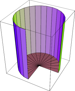
Figure 7: Plot $V(\beta,\gamma)$ of the infinite well potential (25) discussed analytically by Wilets and Jean and and by Iachello with $0<\gamma<3\pi/2$.

With the potential (25) and setting $\varphi(\beta)~{}=~{}\beta^{3/2}f(\beta)$, $z=\beta k$, $k=\sqrt{\varepsilon}$ and $\nu~{}=~{}\tau+3/2$, the $\beta-$part of the Bohr equation may be written as a Bessel equation whose solutions (regular in the origin) are Bessel $J$ function

$$\varphi^{\prime\prime}+{\varphi^{\prime}\over z}+\Bigl{[}1-{(\tau+3/2)^{2}\over z^{2}}\Bigr{]}\varphi~{}=~{}0$$ (37)

with Dirichlet boundary condition ($\varphi(\beta_{w})~{}=~{}0$). This fact determines the spectrum as a function of the $\xi$th zero, $x_{\xi,\tau}$, of the $J_{\tau+3/2}(z)$ function, namely:

$$\varepsilon_{\xi,\tau}~{}=~{}\Biggl{(}{x_{\xi,\tau}\over\beta_{w}}\Biggr{)}^{2}\,.$$ (38)

We display in fig. (8) the lowest part of the spectrum. The wave functions are

$$f_{\xi,\tau}(\beta)~{}=~{}c_{\xi,\tau}\beta^{-3/2}J_{\tau+3/2}\bigl{(}{x_{\xi,\tau}\beta\over\beta_{w}}\bigr{)}\,.$$ (39)

The normalization constant may be found analytically from the normalization condition $\int d\beta\beta^{4}f^{2}(\beta)~{}=~{}1$. The result, containing an hypergeometric function, reads

$${1\over c_{\xi,\tau}^{2}}~{}=~{}{k_{\xi,\tau}^{3+2\tau}\beta_{w}^{2}\over 2^{4+2\tau}}{{}_{1}F_{2}\bigl{(}2+\tau;7/2+\tau,4+2\tau;-k^{2}\bigr{)}\over\Gamma(5/2+\tau)\Gamma(7/2+\tau)}$$ (40)

and, although rather complicated, may furnish an alternative to direct numerical computation.

This extraordinary simple, but nonetheless very successful, solution has been labeled E(5), as the euclidian group in the five dimensional space of the quadrupole variables. This group label may be interpreted in a very straightforward way by noticing that the $\beta-$part eq. (14), and hence eq. (37), may be written as

$$[\pi^{2}+u(\beta)-\varepsilon]f(\beta)=0\,$$ (41)

where $\hat{\pi}^{\mu}$ are the conjugate momenta with respect to the five quadrupole deformation variables, $\hat{\alpha}_{\mu}$. The hamiltonian (41) is invariant with respect to rotations in the five dimensional Hilbert space associated with the variables defined above, and in the special case of the square well either $u(\beta)=0$ or $u(\beta)=\infty$, thus the hamiltonian in the relevant region is written as a function of $\pi$ only (plus a constant). Therefore the hamiltonian is also invariant with respect to translations in the five dimensional space. The present solution is in summary invariant with respect to the transformations induced by the group E(5) that is the semidirect sum of the five dimensional translation and rotation groups.

Figure 8: Spectrum of the five-dimensional infinite square well. Energies are scaled shifting the ground state to zero and fixing the lowest excited $2^{+}$ state to lie at $1$. Transition rates are also reported fixing $B(E2,2_{1,1}\rightarrow 0_{1,0})=100$. Adapted from Iac1

III.5 Caprio’s finite square well solution

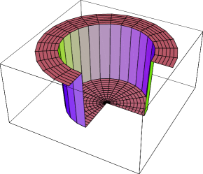
Figure 9: Plot $V(\beta,\gamma)$ of the finite well potential (discussed by Caprio Cap ), with $0<\gamma<3\pi/2$.

The previous analytical solution is a successful approximation of the physics of an entire class of the so-called $\gamma-$unstable nuclei, based on the infinite well potential. Caprio Cap has investigated whether a more realistic behaviour of the potential well, taken as a finite square well, alters this view. The finite square well potential is depicted in fig. 9 and has the following expression

$$V(\beta)~{}=~{}\left\{\begin{array}[]{ccc}V_{0}&,&\beta\leq\beta_{w}\\ 0&,&\beta>\beta_{w}\end{array}\right.$$ (42)

where $\beta_{w}$ is the position of the wall or step. Eigensolutions may be found: inside the well they are again Bessel functions, while outside the well, taking into account the correct asymptotic behaviour at infinity, the solution may be written in terms of modified spherical Bessel functions. The complete solution is

$$f_{\xi,\tau}(\beta)~{}=~{}\left\{\begin{array}[]{ccc}A_{\xi,\tau}\beta^{-1}j_{\tau+1}\big{[}(\epsilon_{\xi,\tau}-v_{0})^{1/2}\beta\big{]}&,&\beta\leq\beta_{w}\\ B_{\xi,\tau}\beta^{-1}k_{\tau+1}\big{[}(-\epsilon_{\xi,\tau})^{1/2}\beta\big{]}&,&\beta>\beta_{w}\end{array}\right.$$ (43)

where $v_{0}=(2B_{m}/\hbar^{2})V_{0}$ is the reduced potential and $\epsilon_{\xi,\tau}$ are the reduced eigenvalues, that are obtained by requiring the continuity of the wave function and of its first derivative at the position of the step $\beta_{w}$. One can define a dimensionless energy variable

$$\eta(\epsilon)\equiv\Bigl{(}1-{\epsilon\over v_{0}}\Bigr{)}^{1/2}$$ (44)

and the parameter

$$x_{0}\equiv\sqrt{-v_{0}}\beta_{w}$$ (45)

and substitute into the matching condition to obtain a transcendental equation that must be solved numerically to determine the eigenvalues.

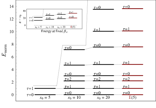
Figure 10: Evolution of excitation energies as a function of $x_{0}$ normalized to the first excited state (absolute energies in the inset). The threshold between bound and unbound states is indicated with a dashed line. Adapted from Cap , courtesy of the author.

Unlike the previous case the spectrum, displayed in fig. 10 has a finite number of discrete eigenvalues, but only those that are lying close to the threshold are appreciably modified with respect to the infinite well solution. For the most part the spectrum does not differ substantially from the E(5) case and the same is true for electromagnetic transition rates.

III.6 Solutions for the Coulomb-like and Kratzer-like potentials

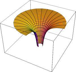
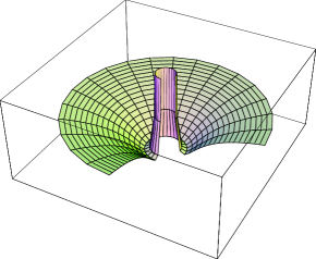
a) b)

Figure 11: Plot $V(\beta,\gamma)$ of the Coulomb-like (a) and Kratzer-like (b) potentials (FV1 ) discussed by Fortunato and Vitturi, with $0<\gamma<3\pi/2$.

The analytic solution of the problem with a Coulomb-like potential (fig. 11, a) and with a Kratzer-like potential (fig. 11, b) has been discussed in ref. FV1 . For these two potentials it is possible to identify the Bohr’s equation with the Whittaker’s equation, whose solution is known in terms of Whittaker’s functions. Namely, after having introduced reduced energies and potential as in the harmonic oscillator case, we can rewrite eq. (15) in its standard form with the transformation $\chi(\beta)=\beta^{2}f(\beta)$. The canonical form for the Bohr equation is thus

$$\chi^{\prime\prime}(\beta)+\Bigl{\{}\epsilon-u(\beta)-{(\tau+3/2)^{2}\over\beta^{2}}+{1\over 4\beta^{2}}\Bigl{\}}\chi(\beta)~{}=~{}0$$ (46)

and will be used in the following to derive analytic solutions in the two cases cited above.

The Coulomb-like potential reads:

$$u_{C}(\beta)=-{A\over\beta}\,,$$ (47)

with $A>0$. With the substitutions $\varepsilon=-\epsilon$, $x=2\sqrt{\varepsilon}\beta$, $k=A/(2\sqrt{\varepsilon})$ and $\mu=\tau+3/2$, equation (46) takes the Whittaker’s standard form Bat :

$$\chi^{\prime\prime}(x)+\Bigl{\{}-{1\over 4}+{k\over x}+{(1/4-\mu^{2})\over x^{2}}\Bigl{\}}\chi(x)~{}=~{}0$$ (48)

and its regular solution for negative energies is (as in Bat ) expressed in terms of the Whittaker’s function $M_{k,\mu}(x)$ :

$$\chi_{k,\mu}(x)~{}=~{}{\cal N}_{\tau,\xi}x^{(2\mu+1)\over 2}e^{-x/2}~{}_{1}F_{1}\bigl{(}\mu+1/2-k,2\mu+1;x\bigr{)}\,.$$ (49)

When the first parameter $\mu+1/2-k=\tau+2-A/(2\sqrt{\varepsilon})$ is a negative integer, that we call $-\xi$, the Whittaker’s function reduces to an associated Laguerre polynomial and the wave function may be written as

$$\chi(x)_{\tau,\xi}={\cal N}_{\tau,\xi}~{}x^{2\mu+1\over 2}e^{-x/2}{\xi!\over(2\mu+1)_{\xi}}L_{\xi}^{(2\mu)}(x)$$ (50)

where the denominator is a Pochhammer symbol. The condition given above fixes analytically the spectrum

$$\varepsilon_{\tau,\xi}={A^{2}/4\over(\tau+\xi+2)^{2}}.$$ (51)

Figure 12: Spectrum of the Coulomb-like potential. The energy scale ($\varepsilon^{\prime}$) is chosen by fixing the energy of the first two states respectively to 0 and 1. The transition rate for $2_{0,1}^{+}\rightarrow 0_{0,0}^{+}$ has been fixed to 100. Some selected quadrupole transitions are shown in the figure for simplicity.

A portion of this spectrum is shown in fig. 12. Its most distinctive features are the position of the $(4^{+},2^{+})$ doublet at an energy of $1.35$ and the presence of a threshold at $1.8$ that corresponds to an infinite quantum number. Note also that each group of $(\xi,\tau)$ states is degenerate with any $(\xi+k,\tau-k)$ group of states with $k=1,...,\tau$.

The Kratzer-like potential may be thought as a modification of the former that may be shaped, adjusting the parameters, in such a way to display a pocket at some fixed point. It has the following expression

$$u_{K}(\beta)=-{A\over\beta}+{B\over\beta^{2}}=-2{\cal D}\Biggl{(}{\beta_{0}\over\beta}-{1\over 2}{\beta_{0}^{2}\over\beta^{2}}\Biggr{)}\,,$$ (52)

where we have shown two possible ways to parameterize this potential. The first is the easiest to use as it will be clear from the formula for the spectrum, while the second is related to the geometrical shape of the potential: ${\cal D}$ is the depth of pocket and $\beta_{0}$ is the position of the minimum. These two sets of parameters are connected by simple relations that may be deduced from the equation above. In the following we shall make use of the former notation. Equation (46) with the Kratzer potential and the substitutions $\varepsilon=-\epsilon$, $x=2\sqrt{\varepsilon}\beta$, $k=A/(2\sqrt{\varepsilon})$ and $\mu^{2}=(\tau+3/2)^{2}+B$, takes again the Whittaker’s standard form. The solutions are the same as above with the new substitutions and the same arguments apply for the properties of convergence. Now $\mu+1/2-k=\sqrt{(\tau+3/2)^{2}+B}+1/2-A/(2\sqrt{\varepsilon})$ must be a negative integer, $-\xi$. The spectrum is in this case:

$$\varepsilon_{\tau,\xi}~{}=~{}{A^{2}/4\over(\sqrt{(\tau+3/2)^{2}+B}+1/2+\xi)^{2}}$$ (53)

with $\xi=0,1,2,..$  to label different families. In reference FV1 the evolution of the spectra with $\beta_{0}$ and ${\cal D}$ is studied in detail in order to establish a connection between shape of the potential and spectrum. Note, however, that if we use the two parameters $A$ and $B$, we can realize that $A$ does not play any role in determining the scaled eigenvalues and therefore the various spectra depend only on $B$, ranging from the Coulomb-like limit ($B=0$) to the O(6) limit ($B\rightarrow\infty$). This is illustrated in fig. (13).

Figure 13: Evolution of spectra with fixed $A=20$ and increasing $B$ for the two limiting situation ($B=0$, Coulomb-like and $B\rightarrow\infty$, O(6) limit). The first two bands ($\xi=0,1$) are displayed with their lowest states ($\tau=0,1,2,..$). The various substates are not displayed for sake of simplicity. Some transition rates are indicated.

The threshold varies with $B$ from $1.8$ to infinity and the position of the $4^{+}$ varies from $1.35$ to $10/3$. This makes the Kratzer-like solution very flexible. The parameter $B$ not only fixes the position of the $4_{0}^{+}$, but also all the other excited states including all the $\beta-$bands.

III.7 Lévai and Arias’ sextic potential solution

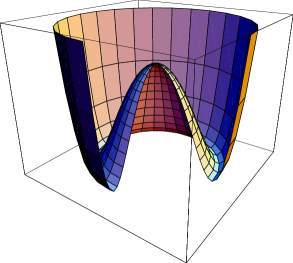
Figure 14: Plot $V(\beta,\gamma)$ with $u^{+}(\beta)$ of the sextic potential discussed by Lévai and Arias Pepe with $0<\gamma<3\pi/2$ for $\tau=0$, $M=1$ and a set of parameters chosen for the purpose of illustration.

J.M.Arias and G.Lévai Pepe proposed the sextic oscillator as an example of quasi-exactly solvable potential for the Bohr hamiltonian. Only a certain number of eigenvalues may be obtained in closed form for this class of potentials. In the present case this is possible for the lowest few values of the principal quantum number. The sextic oscillator has the following expression

$$u^{\pi}(\beta)~{}=~{}(b^{2}-4ac^{\pi})\beta^{2}+2ab\beta^{4}+a^{2}\beta^{6}+u_{0}^{\pi}\,,$$ (54)

where the parameters $a,b$ are used to determine, with an ample choice, the shape of the potential. The index $\pi~{}=~{}\pm$ is used to distinguish between potentials for even and odd values of $\tau$. The constants $c^{\pi}$ are obtained setting $\tau=2s-5/2$ (that must be a non-negative integer) and requiring that

$$s+M+{1\over 2}\equiv c=const.$$ (55)

being $M$ a non-negative integer. For each $M$ it is possible to get analytically $M+1$ of its solutions. The last condition is needed in order to keep constant the quadratic term of the potential, otherwise the shape of the potential will change with $s$. This implies also that when $M$ is increased by one unity, the value of $\tau$ must correspondingly decrease of two units. The constants $u_{0}^{\pi}$ may be used to shift the minima of the two potentials at the same energy. There are various considerations that can be made here, for which the reader is referred to the cited work. For our purpose it will suffice to summarize the solutions in table 3, where the formulae for the lowest eigenvalues are given.

$M$	$\tau$	$n$	$E_{n+1,\tau}$
1	0	$\left.\begin{array}[]{c}0\\ 1\end{array}\right.$	$\left.\begin{array}[]{c}E_{1,0}=7b-2\sqrt{b^{2}+10a}+u_{0}^{+}\\ E_{2,0}=7b+2\sqrt{b^{2}+10a}+u_{0}^{+}\end{array}\right.$
0	2	0	$E_{1,2}=9b+u_{0}^{+}$
1	1	$\left.\begin{array}[]{c}0\\ 1\end{array}\right.$	$\left.\begin{array}[]{c}E_{1,1}=9b-2\sqrt{b^{2}+14a}+u_{0}^{-}\\ E_{2,1}=9b+2\sqrt{b^{2}+14a}+u_{0}^{-}\end{array}\right.$
0	3	0	$E_{1,3}=11b+u_{0}^{-}$

Table 3: Summary of the lowest eigenvalues of the sextic oscillator. For fixed parameters $a,b$ the energies for which a close form may be obtained are labeled by $n$, the number of nodes of the radial wavefunction, and $\tau$.

We give in Fig. (14) an example of the shape of the potential surface in order to help the reader to visualize the sextic potential. This potential is a rather flexible one, since the parameters may be adjusted in order to yield a minimum at $\beta=0$ or at $\beta>0$. In the latter case it might also have a local maximum at some $\beta>0$ before reaching the global minimum. These features may be very useful for an accurate description of shape phase transitions.

The unnormalized solutions of the canonical form of the differential equation (having set $\phi(\beta)=\beta^{2}f(\beta)$) may be written as

$$\phi_{n}(\beta)~{}=~{}P_{n}(\beta^{2})\beta^{2s-1/2}exp\Bigl{(}-{a\beta^{4}\over 4}-{b\beta^{2}\over 2}\Bigr{)}\,,$$ (56)

where $P_{n}$ are polynomials of order $n$. The property of normalizability imposes $a\geq 0$.

III.8 Linear potential

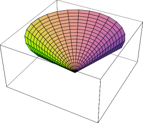
Figure 15: Plot $V(\beta,\gamma)$ of the linear potential with $0<\gamma<3\pi/2$.

We give in this paragraph an approximated treatment à la Wilets et Jean that may be applied to the linear potential

$$u(\beta)=A\beta$$ (57)

being $A$ a positive constant. This is depicted in fig. 15

As far as we know this potential has not been treated in any paper concerning the subject. Regrouping all the terms except the energy in the second term of eq. (46), we can define an effective potential

$$V_{eff}(\beta)=A\beta+{(\tau+3/2)^{2}\over\beta^{2}}-{1\over 4\beta^{2}}$$ (58)

that can be expanded as a Taylor series around the minimum that is located at $\beta_{0}~{}=~{}(2(\tau+1)(\tau+2)/A)^{1/3}$. Neglecting terms of cubic or higher orders, we are now in the conditions to solve the differential equation (analogous to the displaced harmonic oscillator)

$$\chi^{\prime\prime}(\beta)+\Bigl{\{}\epsilon-{3\over 2}A\beta_{0}-{3A\over 2\beta_{0}}(\beta-\beta_{0})^{2}\Bigl{\}}\chi(\beta)~{}=~{}0$$ (59)

that gives the following spectrum:

$$\epsilon_{n_{\beta},\tau}={3\over 2}A\beta_{0}+(n_{\beta}+{1\over 2})\sqrt{3A\over\beta_{0}}.$$ (60)

The wave functions are expressed in terms of Hermite polynomials $H$ of order $n_{\beta}$

$$\chi(\beta)~{}=~{}H_{n_{\beta}}\Bigl{(}(\beta-\beta_{0})\sqrt[4]{3A/\beta_{0}}\Bigr{)}e^{-{(\beta-\beta_{0})^{2}/2\sqrt{3A/\beta_{0}}}}$$ (61)

When one measures, as usual, the energies starting from the ground state in units of the energy of the first $2^{+}$, the spectrum does not depend on the $A$ parameter.

$J^{\pi}$	$n$	$\tau$	approximation	numeric
$0^{+}$	0	0	0	0
$2^{+}$	0	1	1	1
$2,4^{+}$	0	2	1.885	1.911
$3,4,6^{+}$	0	3	2.697	2.755
$4,5,6,8^{+}$	0	4	3.456	3.548
$0^{+}$	1	0	1.466	1.734
$2^{+}$	1	1	2.220	2.568

Table 4: Comparison between approximated eigenvalues calculated with the method explained in the text, and the numerical values courtesy of M.Caprio CapPri . The result is satisfactory for the first family (1 to 3 % errors), while it gets worse, as expected, when $n$ growths.

In table 4 we report a list of the lowest eigenvalues calculated in the present approach (by the author) and numerically by Caprio CapPri . He had performed numerical calculations to check the validity of this approximation as a premise to the so-called sloped wall potential, that is flat from the center to a given point after which it has a linear dependence (see Sect. (III.9.5)).

III.9 Other cases

The cases treated in the previous pages do not exhaust completely the list of known (analytic or approximated) solution, but, to remain loyal to the statements made in the introduction, we preferred to distinguish between the former cases and the present subsection. Solutions of the Bohr hamiltonian have been derived, for instance, from the classical limit of the interacting boson model (IBM). Other potentials, that are interesting for a phenomenological modelization, have been treated numerically. We will briefly examine here some of these cases.

III.9.1 Ginocchio’s anharmonic potential solution

The idea in Ginocchio’s paper Gino , that we will resume without going into the details because it would be a task beyond our aims, is to bridge the IBM and the collective model by means of coherent boson states. Starting from an IBM hamiltonian with anharmonicities (and with a fixed number of bosons) and pairwise interactions he derived a second order differential operator which has a spectrum that contains as the lowest levels the IBM eigenenergies. The radial profile of the potential connected with this solution is very interesting since it is negative in the origin and is very flat near it; it grows rather steadily towards zero at some given point and has a small tail that asymptotically approaches zero. It may be written as

$$V_{A}(\beta)=V_{0}{b\beta^{2}\over 1+b\beta^{2}}\,,$$ (62)

where the strength of the potential is connected to the number of bosons and $b$ measures the anharmonicity of the system. The eigenfunctions are given in terms of Jacobi polynomials:

$$\varphi_{n,\tau}(\beta)=N_{n\tau}(1-x)^{\tau/2}(1+x)^{1+\alpha^{\prime}/2}P_{m}^{\alpha,\alpha^{\prime}}(x)\,,$$ (63)

where $m=(n-\tau)/2$, $\alpha=\tau+3/2$, $\alpha^{\prime}=\bar{N}-n$ and

$$x={1-b\beta^{2}\over 1+b\beta^{2}}\,.$$ (64)

The normalization constant is given by

$$N_{n,\tau}^{2}={b^{5/2}\alpha^{\prime}m!\Gamma(\alpha^{\prime}+\alpha+m+1)\over 2^{\alpha+\alpha^{\prime}-1/2}\Gamma(\alpha+m+1)\Gamma(\alpha^{\prime}+m+1)}\,.$$ (65)

The reader is referred to the original paper and to Ref. Gino2 for details on the normalization, on the volume element, on the eigenenergies, on the additional definitions and on the quantum numbers that find their roots in the IBM.

III.9.2 Warsaw solution

In ref. War1 an interesting $\gamma-$unstable case is solved numerically and compared with data. In particular the so-called Myers-Swiatecki potential:

$$V(\beta^{2})~{}=~{}{1\over 2}V_{c}\beta^{2}+G[e^{-(\beta/a)^{2}}-1]$$ (66)

is solved. With this potential the authors say that they get practically the same results that can be obtained with a modification of the Davidson potential. They also give the analytic solution in this case (about ten years before the work by Elliott and collaborators). This correspondence can be understood, developing the exponential function, from the interplay between the $\beta^{2}$ and $\beta^{-2}$ terms.

In ref. War2 the generalized Bohr hamiltonian is employed (we do not go into details, see GenBo ) with a potential of the following form:

$$V(\beta)~{}=~{}{1\over 2}C_{2}\beta^{2}+C_{8}\beta^{8}+G[e^{-(\beta/a)^{2}}-1]\,.$$ (67)

It is interesting to note that the comparison with the spectrum of ¹³⁴Ba that they obtained is not less valuable that the one obtained in the context of the critical point symmetry E(5). We would like to point out that, if (again) a series expansion for the transcendental function is used, the result is that we have to deal with a generalization of the Davidson potential with even powers of $\beta$. This has been treated in Bona2 where the authors show how the solution of such a potential tend to the infinite square well solution when the leading power increases. They have reasons to believe that a term like $\beta^{8}$ is enough to have a good correspondence.

III.9.3 Quartic potential

The quartic oscillator in $\beta$ is expected to play an important role in the shape phase transition from harmonic oscillator, U(5), to $\gamma-$unstable cases , O(6). In fact it can be shown Pepe2 that the large N limit of the IBM at the critical point and the (numerical) solution of the Bohr differential equation with a $\beta^{4}$ potential lead to the same results and these results are fundamentally different from the analytic solution obtained from the solution of the Bohr equation with an infinite square well, the so called E(5) symmetry. Thus it should be stressed that E(5) symmetry is the exact mathematical solution for an approximate physical problem. In table 5 we give numerical values for the excitation energies of the $\beta^{4}$ potential and we refer to Pepe2 for a thorough comparison with E(5).

	$\xi=1$	$\xi=2$	$\xi=3$	$\xi=4$
$\tau=0$	0.00	2.39	5.15	8.20
$\tau=1$	1.00	3.63	6.56	9.75
$\tau=2$	2.09	4.92	8.01	11.34
$\tau=3$	3.27	6.26	9.50	12.95

Table 5: Excitation energies for a $\beta^{4}$ potential relative to the energy of the first excited state (from Pepe2 ).

They obtain a geometrical limit of IBM by using a coherent state formalism. Considering two different IBM hamiltonian they obtain energy surfaces showing that a $\beta^{4}$ potential is associated with the critical point. It is also argued that the IBM could provide the finite N correction to the predictions of the simple collective model. This is of interest for an identification of nuclei at the critical point.

III.9.4 Bonatsos’ et al. solution

A study that deserves comments is a generalization of the harmonic oscillator and quartic potentials that has been discussed in Bona1 . The authors solve numerically the Bohr hamiltonian with the sequence of potential $\beta^{2n}$ with $n$ positive non-null integer.

The harmonic oscillator case occurs for $n=1$, while the square well may be considered as the limit for $n\rightarrow\infty$. The structure of the spectra of all these potentials changes smoothly from one extreme to the other, thus bridging the two solutions. This model allows thus for a large variety of different spectra with the $R_{4/2}$ ratio varying from $2$ to $2.20$.

III.9.5 Caprio’s sloped wall potential

The E(5) and X(5) solutions generated not only an experimental effort aimed at the recognition of new patterns in nuclear spectra, but also a theoretical effort aimed at the assessment of its most important characteristics. The solution for the finite square well and the solution for the sloped wall potential are parts of this effort. In the former case the conclusion was that the results of the E(5) model are quite robust with respect to the introduction of a finite depth. In the latter case a flat potential with a sloped wall was investigated Capslo to establish if the results of the E(5) and X(5) symmetries are robust with respect to (small) inclinations of the wall of the infinite potential well. The sloped-wall potential reads:

$$V(\beta)~{}=~{}\left\{\begin{array}[]{ccc}V_{0}&,&\beta\leq\beta_{w}\\ C(\beta-\beta_{w})&,&\beta>\beta_{w}\end{array}\right.\,.$$ (68)

The solution in the internal region may be found analytically in terms of Bessel function, while in the external region an analytic treatment is not possible. The author notice that when the term with a $\beta^{-2}$ dependence is not present, the equation in $\beta$ reduces to the Airy equation for which the solution is possible. The problem is then solved numerically using the Airy functions as an efficient basis for diagonalization. The eigenvalues are determined by the condition of continuity of the logarithmic derivative at the matching point. The eigenvalues are lowered relative to the respective infinite square well cases, and the lowering is more effective for high lying states. On the whole the spectrum is very sensitive to the stiffness of the wall, and the deviation from the X(5) predictions are able to generate a closer agreement with nuclear spectra in the $N\sim 90$ region.

IV Axial $\gamma-$stable cases.

The present section deals mainly with potentials of the type $u(\beta,\gamma)~{}=~{}u(\beta)+v(\gamma)$, where the term in $\gamma$ is taken as an harmonic oscillator. This clearly violates the property of periodicity in $\gamma$ that our problem possesses. However if we consider only a narrow interval of $\gamma$’s around zero it is possible to give an analytic solution to the differential equations using the expansion of the periodic functions around $\gamma=0$ (see for example Wilet for a thorough analysis). Although this is not the only possibility to obtain solvable, or approximatively solvable, Bohr hamiltonians, we will discuss it in detail for its importance in connection with the issue of critical point symmetries and shape phase transitions. This was first discussed in ref. Iac2 , where the approximations that will be used throughout were introduced. Within this class of potentials one may study approximate solutions for a $\beta-$soft, $\gamma-$soft rotor. In subsection E a different method, that leads to an exact separation, is used.

It is perhaps worth saying that when the $\gamma$ degree of freedom comes into play, one usually have to consider $\gamma$ phonons. The $\beta$ phonon shares the same total angular momentum ($\lambda=2$) with the $\gamma$ phonon, but while the former has a null component along the quantization axis, the latter has a non null ($\mu=\pm 2$) component. The rules to assign quantum numbers to the various states, for a given number of quanta in $\gamma$, are:

$$j=0,...,n_{\gamma}$$

$$K=2n_{\gamma}-4j$$

$$L=\left\{\begin{array}[]{rr}0,2,4,6,8,...{}{}{}{}{}{}{}{}&K=0\\ K,K+1,K+2,...&K\neq 0\end{array}\right.$$ (69)

When $K$ is negative one must consider its absolute value.

IV.1 Iachello’s square well solution or X(5)

This important case gave the starting signal to a number of experimental works about the so-called X(5) symmetry. Iachello proposed an approximate separation of variables for the Bohr hamiltonian that consists of two steps. The first point is to realize that around $\gamma~{}=~{}0^{o}$ the rotational kinetic energy, eq. (12), may be written as

$$\sum_{k=1}^{3}{{\hat{Q}}_{k}^{2}\over\sin{\bigl{(}\gamma-{2\pi\over 3}k}\bigr{)}^{2}}\simeq{4\over 3}(\underbrace{{\hat{Q}}_{1}^{2}+{\hat{Q}}_{2}^{2}+{\hat{Q}}_{3}^{2}}_{L^{2}})+{\hat{Q}}_{3}^{2}\Bigl{(}{1\over\sin{\gamma}^{2}}-{4\over 3}\Bigr{)}\,.$$ (70)

In this case the problem is no longer $\gamma-$unstable and the separation of the wavefunction á la Bes do not hold anymore. We should instead look for solutions of the type $\Psi(\beta,\gamma,\theta_{i})~{}=~{}\varphi_{K}^{L}(\beta,\gamma){\cal D}_{M,K}^{L}(\theta_{i})$, where ${\cal D}$ is a Wigner function, eigenfunction of the square of total angular momentum and of its third component. The action of $L^{2}$ and ${\hat{Q}}_{3}^{2}$ leaves the following equation

$$\Biggl{\{}-{1\over\beta^{4}}{\partial\over\partial\beta}\beta^{4}{\partial\over\partial\beta}-{1\over\beta^{2}}{1\over\sin{3\gamma}}{\partial\over\partial\gamma}\sin{3\gamma}{\partial\over\partial\gamma}+{1\over 4\beta^{2}}\Biggl{[}{4\over 3}L(L+1)+K^{2}\Bigl{(}{1\over\sin{\gamma}^{2}}-{4\over 3}\Bigr{)}\Biggr{]}+u(\beta,\gamma)\Biggr{\}}\varphi_{K}^{L}(\beta,\gamma)~{}=~{}\epsilon\varphi_{K}^{L}(\beta,\gamma)\,.$$ (71)

Considering now a potential of the type $u(\beta,\gamma)~{}=~{}u(\beta)+v(\gamma)$ the above equation may be approximately separated into the following set

$$\Biggl{[}-{1\over\beta^{4}}{\partial\over\partial\beta}\beta^{4}{\partial\over\partial\beta}+{L(L+1)\over 3\beta^{2}}+u(\beta)\Biggr{]}\xi_{L}(\beta)~{}=~{}\epsilon_{\beta}\xi_{L}(\beta)$$ (72)

$$\Biggl{[}-{1\over\langle\beta^{2}\rangle\sin{3\gamma}}{\partial\over\partial\gamma}\sin{3\gamma}{\partial\over\partial\gamma}+{1\over 4\langle\beta^{2}\rangle}K^{2}\Biggl{(}{1\over\sin{\gamma}^{2}}-{4\over 3}\Biggr{)}+v(\gamma)\Biggr{]}\eta_{K}(\gamma)~{}=~{}\epsilon_{\gamma}\eta_{K}(\gamma)\,,$$ (73)

where $\langle\beta^{2}\rangle$ is the average of $\beta^{2}$ over $\xi(\beta)$. Here we have $\epsilon\simeq\epsilon_{\beta}+\epsilon_{\gamma}$ and $\varphi_{K}^{L}(\beta,\gamma)\simeq\xi_{L}(\beta)\eta_{K}(\gamma)$. Some authors noticed that a different set of equations, in which the term $K^{2}/(3\langle\beta^{2}\rangle)$ is kept in the first equation, may have been derived as well. In this case, that we will not take into account, the solution of the $\beta$ equation would carry also the $K$ quantum number.

Insofar the procedure has been carried for a general potential. Iachello treated a square well potential in $\beta$ combined with a harmonic oscillator in $\gamma$. Introducing the square well potential (25) into eq. (72) and setting $\tilde{\xi}(\beta)=\beta^{3/2}\xi(\beta)$, $\epsilon_{\beta}=k_{\beta}^{2}$ and $z=\beta k_{\beta}$, he obtained a Bessel equation

$$\tilde{\xi}^{\prime\prime}+{\tilde{\xi}^{\prime}\over z}+\Biggl{[}1-{\nu^{2}\over z^{2}}\Biggr{]}\tilde{\xi}~{}=~{}0\,,$$ (74)

where

$$\nu~{}=~{}\Bigl{(}{L(L+1)\over 3}+{9\over 4}\Bigr{)}^{1/2}~{}~{}.$$ (75)

The solution of this equation is therefore expressed in terms of Bessel function with a non-integer index, $\nu$,

$$\xi_{s,L}~{}=~{}c_{s,L}\beta^{-3/2}J_{\nu}(k_{s,L}\beta)\,,$$ (76)

where the set of quantum numbers refers to the $s$th zero of the Bessel function $J_{\nu}(z)$ and to the total angular momentum, $L$. In fact the boundary condition at the wall of the well, $\tilde{\xi}(\beta_{w})~{}=~{}0$, determines the eigenvalues, because the wave function has a node if and only if the Bessel function has a zero, that we call $x_{s,L}$. The spectrum is thus

$$\epsilon_{s,L}~{}=~{}(k_{s,L})^{2}\,,$$ (77)

where $k_{s,L}~{}=~{}{x_{s,L}\over\beta_{w}}$ and $\beta_{w}$ is the position of the wall.

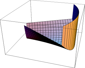
Figure 16: Plot $V(\beta,\gamma)$ of the square well potential in $\beta$ combined with a harmonic oscillator in $\gamma$ discussed by Iachello, with $-\pi/4<\gamma<\pi/4$.

We give here the solution of the $\gamma-$part for the harmonic oscillator, as it was given by Iachello. The following subsections IV.2 - IV.4 will share the same treatment for the $\gamma-$variable. A trigonometric expansion, strictly valid in a small sector around the origin ($\sin{\gamma}\sim\gamma$), is made in eq. (73) with a harmonic oscillator potential, obtaining formally the radial equation of a two dimensional harmonic oscillator:

$$\Bigl{[}-{1\over\langle\beta^{2}\rangle}{1\over\gamma}{\partial\over\partial\gamma}\gamma{\partial\over\partial\gamma}+{K^{2}\over 4\langle\beta^{2}\rangle}{1\over\gamma^{2}}+(3a)^{2}{\gamma^{2}\over 2}\Bigr{]}\eta_{K}(\gamma)~{}=~{}{\tilde{\varepsilon}}_{\gamma}\eta_{K}(\gamma)\,,$$ (78)

with ${\tilde{\varepsilon}}_{\gamma}~{}=~{}\varepsilon_{\gamma}+{K^{2}\over 3\langle\beta^{2}\rangle}$. The solution is given by

$${\tilde{\varepsilon}}_{\gamma}~{}=~{}{3a\over\sqrt{\langle\beta^{2}\rangle}}(n_{\gamma}+1)$$ (79)

and

$$\eta_{n_{\gamma},K}(\gamma)~{}=~{}c_{n,K}\gamma^{\mid K/2\mid}e^{-3a\gamma^{2}/2}L_{n}^{\mid K\mid}(3a\gamma^{2})\,,$$ (80)

where $n=(n_{\gamma}-\mid K\mid)/2$ with $n_{\gamma}=0,1,2,\ldots~{}$ and $L_{n}^{\mid K\mid}$ are Laguerre polynomials. The parameter $a$ is the strength of the harmonic oscillator potential, or in other words its amplitude.

IV.2 Solutions for Coulomb- and Kratzer-like potentials

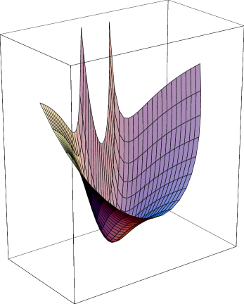
Figure 17: Plot $V(\beta,\gamma)$ of the Kratzer-like potential (FV2 ) combined with a harmonic oscillator in $\gamma$ discussed by Fortunato and Vitturi, with $-\pi/6<\gamma<\pi/6$.

With the substitution $\xi_{L}(\beta)~{}=~{}\chi_{L}(\beta)\beta^{-2}$, equation (72) may be simplified to its standard form:

$${\partial^{2}\over\partial\beta^{2}}\chi_{L}(\beta)+\Biggl{\{}\varepsilon^{(\beta)}-u(\beta)-\Biggl{(}{2+{L(L+1)\over 3}\over\beta^{2}}\Biggr{)}\Biggr{\}}\chi_{L}(\beta)~{}=~{}0\,.$$ (81)

By inserting the Coulomb-like potential $u(\beta)~{}=~{}-A/\beta$ with $A>0$ and recasting the problem in the variable $x~{}=~{}2\beta\sqrt{\epsilon}$, with the further substitutions $\varepsilon~{}=~{}-\epsilon$, $k={A\over 2\sqrt{\epsilon}}$ and $\mu^{2}=\bigl{(}{9\over 4}+{L(L+1)\over 3}\bigr{)}$, we obtain the Whittaker’s equation

$${\partial^{2}\over\partial x^{2}}\chi_{L}(x)+\Biggl{\{}-{1\over 4}+{k\over x}+{1/4-\mu^{2}\over x^{2}}\Biggr{\}}\chi_{L}(x)~{}=~{}0\,.$$ (82)

Its regular solution is the Whittaker function $M_{k,\mu}(x)$ that reads:

$$\chi_{L}(x)~{}=~{}{\cal N}e^{-x/2}x^{{1\over 2}+\mu}~{}_{1}F_{1}\bigl{(}{1\over 2}+\mu-k,1+2\mu,x\bigr{)}$$ (83)

which is, in general, a multivalued function. The constant ${\cal N}$ is determined from the normalization condition. We adopt usual conventions and thus the function is analytic on the real axis. The hypergeometric series is an infinite series and to recover a good asymptotic behaviour we must require that it terminates, i.e. that it becomes a polynomial. This happens when the first argument is a negative integer, $-v$, that must thence be regarded as an additive quantum number. This condition fixes unambiguously the $\beta$ part of the spectrum:

$$\epsilon_{v,L}^{(\beta)}~{}=~{}{A^{2}/4\over\Biggl{(}\sqrt{{9\over 4}+{L(L+1)\over 3}}+{1\over 2}+v\Biggr{)}^{2}}\,.$$ (84)

Figure 18: $\beta-$spectrum of the Coulomb-like case ($n_{\gamma}=0$). The vertical scale is expressed in units of the energy of the $(v=0,L=2)$ state. Some B(E2) values are displayed in units of the lowest transition of the first band (numbers in italics). Notice the presence and energy of a threshold and the absence of degeneracy. From FV2 .

Fig. 18 shows the spectrum of the axial rotor with coulomb-like potential.

The case of the Kratzer-like potential is treated in a very similar way. Inserting in eq. (81) the potential

$$u(\beta)=-A/\beta+B/\beta^{2}$$ (85)

and setting $x~{}=~{}2\beta\sqrt{\epsilon}$, $\varepsilon~{}=~{}-\epsilon$, $k={A\over 2\sqrt{\epsilon}}$ and $\mu^{2}=\bigl{(}B+{9\over 4}+{L(L+1)\over 3}\bigr{)}$, we obtain again the Whittaker’s equation whose solutions may be written as in eq. (83) and we may repeat the whole procedure of the previous section, the only major difference being the definition of $\mu$. The spectrum assumes in this case the form

$$\epsilon_{v,L}^{(\beta)}~{}=~{}{A^{2}/4\over\Biggl{(}\sqrt{B+{9\over 4}+{L(L+1)\over 3}}+{1\over 2}+v\Biggr{)}^{2}}~{}.$$ (86)

We recall (see sect. III.6) that the two parameters used here, $A$ and $B$, have an immediate translation into the position, $\beta_{0}$, and depth of the minimum of the potential, ${\cal D}$, being valid the following relations: $A~{}=~{}2\beta_{0}{\cal D}$ and $B~{}=~{}\beta_{0}^{2}{\cal D}$. Consequently $\beta_{0}~{}=~{}2B/A$ and ${\cal D}~{}=~{}A^{2}/(4B)$.

Figure 19: Evolution of the $\beta-$spectrum of the Kratzer-like rotor with the parameter $B$. The vertical scale is expressed in units of the energy of the $(v=0,L=2)$ state. The B(E2) values, calculated with formula (LABEL:be2), between the lowest states are indicated in italics beside the corresponding downward arrows. Intraband transitions are not marked for the sake of simplicity. From FV2 .

In fig. 19 we report a study of the evolution of the spectrum and transition rates for the Kratzer-like rotor as a function of the parameter $B$. When $B$ is large a typical rotational spectrum is recovered.

IV.3 Bonatsos’ et al. solution

As in sec. III.9.4, we summarize here briefly another work by Bonatsos and collaborators Bona2 that deals with the numerical solution of a sequence of potentials interpolating between the U(5) and X(5) models of the form:

$$u_{2n}(\beta,\gamma)~{}=~{}{\beta^{2n}\over 2}+c\gamma^{2}\,,$$ (87)

where the harmonic dependence on $\gamma$ is the same of the X(5) case, while the potential in $\beta$ may be considered as a generalization of other cases. For $n=1$ one gets an exactly soluble model that is called X(5)$-\beta^{2}$, while for $n\rightarrow\infty$ the infinite square well potential is recovered. As expected energy ratios and transition rated change smoothly from one limiting case to the other and it is shown that the X(5) results are already well approximated for $n\sim 4$.

IV.4 Pietralla and Gorbachenko’s solution or CBS-model

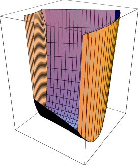
Figure 20: Plot $V(\beta,\gamma)$ of the two-sided infinite square well potential in $\beta$ combined with a harmonic oscillator in $\gamma$ discussed by Pietralla and Gorbachenko Pietr , with $-\pi/12<\gamma<\pi/6$.

An extension of the X(5) model has been recently proposed Pietr with the aim to study the evolution of the first excited $0^{+}$ state in transitional nuclei ($N\sim 90$). The authors consider the same problem discussed by Iachello for axially symmetric prolate nuclei, but they take as a potential in $\beta$ the infinite square well with two boundaries:

$$V(\beta)~{}=~{}\left\{\begin{array}[]{ccc}\infty&,&\beta<\beta_{m}\\ 0&,&\beta_{m}\leq\beta<\beta_{M}\\ \infty&,&\beta\geq\beta_{M}\end{array}\right.$$ (88)

The number $r_{\beta}=\beta_{m}/\beta_{M}$ may be used to parameterize the stiffness of the potential. The X(5) solution is a special case of this model for $r_{\beta}=0$ as well as the rigid rotor is another special case for $r_{\beta}=1$. Eq. (72) may be transformed into the Bessel equation with the substitutions $z=\sqrt{E/(\hbar^{2}/2B_{m})}\beta$ and $\tilde{\xi}(z)=\beta^{3/2}\xi_{L}(\beta)$. The solution is a linear combination of Bessel’s $J_{\nu}(z)$ and $Y_{\nu}(z)$ functions with index $\nu=\sqrt{L(L+1)/3+9/4}$. The authors give the complete solution in the following form:

$$\xi_{L,s}(\beta)={c_{L,s}\over\beta^{3/2}}\Bigl{[}J_{\nu}\bigl{(}z_{L,s}^{r_{\beta}}\beta/\beta_{M}\bigr{)}+\gamma_{Y}Y_{\nu}\bigl{(}z_{L,s}^{r_{\beta}}\beta/\beta_{M}\bigr{)}\Bigr{]}\,,$$ (89)

where $c_{L,s}$ is a normalization constant. The spectrum is found imposing the condition that the wave functions in $\beta$ must have nodes at the two boundaries:

$$\xi(\beta_{m})=\xi(\beta_{M})=0$$

or

$$\tilde{\xi}(r_{\beta}z_{m})=\tilde{\xi}(z_{M})=0\,,$$ (90)

where $z_{M}=\sqrt{E/(\hbar^{2}/2B_{m})}\beta_{M}$. The quantization condition is thus

$$J_{\nu}(z_{M})Y_{\nu}(r_{\beta}z_{M})-J_{\nu}(r_{\beta}z_{M})Y_{\nu}(z_{M})=0\,,$$ (91)

whose $s$th zero, $z_{L,s}^{r_{\beta}}$, must be calculated numerically. The eigenvalues are found as

$$E_{L,s}={\hbar^{2}\over 2B_{m}\beta_{M}^{2}}(z_{L,s}^{r_{\beta}})^{2}\,.$$ (92)

This solution is rather interesting because there is one more degree of freedom with respect to X(5) and moving $r_{\beta}$ from 0 to 1 has not only the effect of increasing the position of the $\beta$ bands, but also to invert the trend of the ratio $R_{4/2}(s)$: while for $r_{\beta}=0$ the ratio $R_{4/2}$ of the ground state band is higher than for any excited band, for greater values of $r_{\beta}$ the opposite happens. Another interesting feature of this model is the possibility to study the effect of the ’centrifugal stretching’: the term with $\beta^{-2}$ power acts as a ’centrifugal stretch’ (although for the sake of clarity the variable here is not the radius of the system, but its deformation) in the sense that the wave functions of states labeled by high values of the SO(6) quantum number will be pushed towards higher deformations, decreasing their probability amplitudes in the region close to the origin. Within this model one actually cut the region close to the origin with the internal wall. As a consequence only states with appreciable amplitude in the classically forbidden area will be more affected: the overall result is that states with high $\tau$ are not much affected by the presence of the internal wall, while states with low $\tau$ are shifted up in energy. The spectrum will therefore show smaller energy distances among low-lying states with respect to X(5).

The authors named their model as ”confined $\beta-$soft” rotor model (CBS) by analogy with the Wilets-Jean $\gamma-$soft model (see Appendix B).

IV.5 Prolate and oblate axial rotor: new cases

We propose in this section new solutions that, as far as we know, have not been published anywhere else, although they are pretty simple. To obtain them we have done nothing but collecting knowledge coming from the various solutions that have been devised so far and apply known approximations. In doing so we made use of some suggestions due to D.J.Rowe RoPR . The novelty here is represented by the transformation (97) that allows a better level of approximation for the goniometric functions. This is reflected in four new analytically solvable cases.

The Schrödinger equation for the Bohr hamiltonian may be profitably simplified for the prolate and oblate soft axial rotors (respectively around $\gamma\sim 0$ and around $\gamma\sim\pi$) using the approximation (70) devised by Iachello. Alternatively one can treat the $\gamma\sim\pi/3$ case by noticing that in that case the projection of the angular momentum on the intrinsic x-axis is a good quantum number (see fig. 1). We will seek solutions of the type

$$\Psi(\beta,\gamma\theta_{i})=\xi_{L}(\beta)\eta_{K}(\gamma){\cal D}^{L}_{M,K}(\theta_{i})\,.$$ (93)

Since the rotational part is standard and the action of the square of the angular momentum and of its third component are trivially evaluated, we will restrict to the $\beta-\gamma$ part, as done in Iac2 . The result is formula (71), that we employ here as a starting point for new solutions.

Contrary to what was done in the X(5) model Iac2 , we may separate exactly the Bohr equation as explained in section V.4, using a potential of the form $u(\beta,\gamma)~{}=~{}u_{1}(\beta)+u_{2}(\gamma)/\beta^{2}$, obtaining the following two equations

$$\Biggl{\{}-{1\over\beta^{4}}{\partial\over\partial\beta}\beta^{4}{\partial\over\partial\beta}+u_{1}(\beta)-\epsilon+{\omega+{L(L+1)-K^{2}\over 3}\over\beta^{2}}\Biggr{\}}\xi_{L,K}(\beta)~{}=~{}0$$ (94)

$$\Biggl{\{}-{1\over\sin{(3\gamma)}}{\partial\over\partial\gamma}\sin{(3\gamma)}{\partial\over\partial\gamma}+{K^{2}\over 4\sin{(\gamma)}^{2}}+u_{2}(\gamma)-\omega\Biggr{\}}\eta_{K}(\gamma)~{}=~{}0$$ (95)

where $\omega$ is a separation constant and the energy, $\epsilon$, is contained only in the first equation. Notice that one could have alternatively retained one or both of the terms $L(L+1)/3$ and $K^{2}/3$ in the equation for $\gamma$. We prefer to keep them in the $\beta-$part because this part is solved exactly. The $\gamma-$part usually experiences a second turn of approximations.

In the second equation one can adopt the same trigonometric simplifications ($\sin{\gamma}\sim\gamma$ and $\cos{\gamma}\sim 1$) that are implicitly used in (70) or may try a more sophisticated approach. In fact eq. (95) may be written as

$$\Biggl{\{}{\partial^{2}\over\partial\gamma^{2}}+3\cot{3\gamma}{\partial\over\partial\gamma}+\omega-u_{2}(\gamma)-{K^{2}\over 4\sin^{2}{(\gamma)}}\Biggr{\}}\eta_{K}(\gamma)=0$$ (96)

and with the transformation

$$\eta_{K}(\gamma)={\rho_{K}(\gamma)\over\sqrt{\sin{3\gamma}}}$$ (97)

it may be brought in the standard form

$$\Biggl{\{}{\partial^{2}\over\partial\gamma^{2}}+\omega-u_{2}(\gamma)+{9\over 2}-{K^{2}\over 4\sin^{2}{\gamma}}+{9\over 4}\cot^{2}{(3\gamma)}\Biggr{\}}\rho_{K}(\gamma)=0\,,$$ (98)

where the term with the first derivative has been eliminated. It is worth noticing that now a better approximation may be used for the trigonometric functions, without loosing the possibility to solve exactly the equation. The series expansion for the cotangent, including the second order, may be used

$${9\over 4}\cot^{2}(3\gamma)\sim{1\over 4\gamma^{2}}-{3\over 2}+{27\over 20}\gamma^{2}\,.$$ (99)

Therefore we can recast the differential equation above as

$$\Biggl{\{}{\partial^{2}\over\partial\gamma^{2}}+\underbrace{\omega+3}_{q^{2}}+{27\over 20}\gamma^{2}-u_{2}(\gamma)+{1-K^{2}\over 4\gamma^{2}}\Biggr{\}}\rho_{K}(\gamma)=0\,.$$ (100)

This expression represents a better level of approximation with respect to any equation used so far for the $\gamma$ part of the problem. The ’extra’ term with dependence $\gamma^{-2}$ has the same behaviour of a ’centrifugal’ term and the differential equation can be solved exactly with harmonic or Davidson potentials for $u_{2}(\gamma)$.

With $u_{2}(\gamma)=C\gamma^{2}$, defining $\mu=q^{2}/(2\lambda)$ and $\lambda^{2}=C-{27\over 20}$ and $t(t+1)=(K^{2}-1)/4$ we obtain

$$\rho_{K}(\gamma)={\cal N}\gamma^{t+1}e^{-{\lambda\over 2}\gamma^{2}}~{}_{1}F_{1}\Bigl{(}{t+3/2-\mu\over 2},t+3/2;\lambda\gamma^{2}\Bigr{)}\,,$$ (101)

where the confluent hypergeometric function is not divergent only when it is a polynomial: this happens if the first argument is equal to $-n_{\gamma}$ with $n_{\gamma}=0,1,2,3,...$. This requirement sets the formula for the spectrum

$$\omega_{n_{\gamma},K}=\sqrt{C-{27\over 20}}\Bigl{(}2t+3+4n_{\gamma}\Bigr{)}-3\,.$$ (102)

Notice the constraint on the value of $C$ that comes from the square root. With

$$t={-1\pm\mid K\mid\over 2}$$ (103)

we can write

$$\omega_{n_{\gamma},K}=\sqrt{C-{27\over 20}}\Bigl{(}\pm\mid K\mid+2+4n_{\gamma}\Bigr{)}-3\,.$$ (104)

The structure of the various bands predicted by this formula is depicted in fig. 21. We shifted the energies eliminating the term $-3$ and we used a constant strength ($\lambda$) equal to unity for purpose of illustration.

Figure 21: Graphical representation of the values of $\omega_{n_{\gamma},K}$ for the lowest states of a few bands, obtained from formula (104) with $\lambda=1$ (the shift, $-3$, has been omitted). The assignation of quantum numbers to each band follows from (69).

The expression for $\omega$ must be now used inside the equation for the $\beta$ part. Choosing for example the harmonic oscillator: $u_{1}(\beta)=k\beta^{2}$ one has:

$$\epsilon=\sqrt{k}\bigl{(}2n_{\beta}+\tau+5/2\bigr{)}$$ (105)

with $\tau$ is determined through the relation

$$\tau(\tau+3)=\omega_{n_{\gamma},K}+{L(L+1)-K^{2}\over 3}$$ (106)

(one can employ the Davidson potential in a very similar way). Alternatively we may consider the Coulomb potential, $u_{1}(\beta)=-A/\beta$, or the Kratzer potential, $u_{1}(\beta)=-A/\beta+B/\beta^{2}$. In the latter more general case we obtained

$$\epsilon={A^{2}/4\over\Bigl{(}\sqrt{1/4+B+\omega_{n_{\gamma},K}+{L(L+1)-K^{2}\over 3}}+1/2+n_{\beta}\Bigr{)}^{2}}\,,$$ (107)

where one should insert the values of $\omega$ previously found in formula (104). The most relevant implication of this model is the difference between bands with opposites signs of $K$.

V Triaxial cases

We divided this section from the previous one, although they both deal with $\gamma-$stable cases, because in triaxial nuclei the minimum of the potential along $\gamma$ is not located at $n{\pi\over 3}$, with $n\in\mathbb{Z}$. This implies the absence of axial symmetry.

In triaxial nuclei the eigenvalue of the projection of the third component of the angular momentum is no more a good quantum number (this can be seen already at the classical level). In the special case of $\gamma=30^{o}$ the projection of the angular momentum on the intrinsic y-axis, called sometimes $R$, is a conserved quantity, but in the regions $0^{o}<\gamma<30^{o}$ and $30^{o}<\gamma<60^{o}$ is not possible to use $K$ or $R$ to label bands. Notice that in the axial case the lowest member of a group of states with the same $L$ has always the lowest possible value of $K$, while at $\gamma=30^{o}$ the lowest state with a given $L$ has the highest possible value of $R$ (this is a trivial consequence of formula (116)).

V.1 Davydov’s classical solution or rigid rotor model

Traditionally the name of Davydov is associated with a series of papers Dav1 ; Dav2 ; Dav3 ; Dav4 in collaboration with other various researchers. Davydov and Filippov proposed the existence of triaxial nuclei, the properties of which have been investigated in the adiabatic approximation, which assumes rotation of the nucleus without change of the intrinsic state. The equilibrium shape is a triaxial ellipsoid, whose hamiltonian, frequently called the rigid rotor hamiltonian, may be written as:

$$H={1\over 2}\sum_{\kappa=1}^{3}{{\hat{Q}}_{\kappa}^{2}\over\sin{(\gamma-{2\over 3}\pi\kappa)}^{2}}\,,$$ (108)

where ${\hat{Q}}_{\lambda}$ are the projections of the total angular momentum operator on the axes of the intrinsic system. The wave functions are expanded in terms of (axial) rotational wave functions

$$\Psi_{JM}=\sum_{K}\mid JK\rangle A_{K}\,,$$ (109)

with

$$\mid JK\rangle=\sqrt{2J+1\over 16\pi^{2}(1+\delta_{K0})}\Bigl{(}{\cal D}_{M,K}^{J}+(-)^{J}{\cal D}_{M,-K}^{J}\Bigr{)}\,,$$ (110)

where $K=0,2,4,...$ and

$$J=\left\{\begin{array}[]{lc}K,K+1,K+2,...&K\neq 0\\ 0,2,4,...&K=0\end{array}\right.\,.$$ (111)

Within this rigid-rotor approach analytic expressions may be derived for a few rotational levels with low total angular momentum, although this model completely neglects the shape vibrational degrees of freedom.

A more complicated version, containing the kinetic energy in the $\beta$ variable along with the above rigid rotor hamiltonian and a potential term $V(\beta)$ may be employed Dav3 . The corresponding Schrödinger equation for this $\gamma-$rigid, $\beta-$soft model is separable and leads to lengthy expressions for the energy of collective nuclear states. We give here a simplified version of the spectrum:

$$E_{J,K,n_{\beta}}=(n_{\beta}+1/2)E_{\beta}+c_{1}(J(J+1)-K^{2})+c_{2}K^{2}\,,$$ (112)

where $n_{\beta}=0,1,2,..$ is the number of $\beta$ phonons.

Davydov proposed also a solution that takes into account $\beta$ and $\gamma$ vibrations. When in the Bohr hamiltonian a potential of the type

$$V(\beta,\gamma)={1\over 2}C(\beta-\beta_{0})^{2}+{1\over 2}C_{\gamma}\beta_{0}^{2}(\gamma-\gamma_{0})^{2}$$ (113)

is employed, we can look for solutions that are product of $f(\beta)$ and $\Phi(\gamma,\theta_{i})$ functions, obeying the following equations:

$$\Bigl{(}-{1\over\sin{3\gamma}}{\partial\over\partial\gamma}\sin{3\gamma}{\partial\over\partial\gamma}+{1\over 4}\sum_{\kappa=1}^{3}{{\hat{Q}_{\kappa}}^{2}\over\sin{(\gamma-{2\over 3}\pi\kappa)}^{2}}+D(\gamma-\gamma_{0})^{2}-\Lambda\Bigr{)}\Phi(\gamma,\theta_{i})=0$$ (114)

and

$$\Bigl{[}-{\hbar^{2}\over 2B_{m}}{d^{2}\over d\beta^{2}}+{1\over 2}C(\beta-\beta_{0})^{2}+{\hbar^{2}(\Lambda+2)\over 2B\beta^{2}}-E\Bigr{]}\beta^{2}f(\beta)=0\,,$$ (115)

where $C_{\gamma}~{}=~{}\omega_{\gamma}^{2}B$ contains the frequency of the $\gamma$ vibration.

The above equations can be solved exactly for a spherical nucleus, reproducing known results. Davydov proposed also a solution for non-axial nuclei when small oscillations around the equilibrium position are considered. The main point is to approximate the effective potential, that consists of the displaced harmonic oscillator and the ’centrifugal’ term, expanding it as a power series as Wilets and Jean did for the $\gamma-$unstable case. In the present approach (as in the previous one, that has only $\beta$ vibrations) a rather complicated expression for the energy levels is found that accounts for rotations as well as $\beta$ and $\gamma$ vibrations. Although we do not enter into the details, it should be said that this approach had considerable success and applications to nuclear spectra.

V.2 Meyer-ter-vehn formula

In a work focused on the spectrum of an odd nucleon coupled with a rotating triaxial core MTV , Meyer-ter-vehn introduced also a simple analytic formula for the spectrum of the rigid rotor at $\gamma=30^{o}$. At that angle two of the three moment of inertia are equal (albeit the axis of the ellipsoid does not have equal length) and the hamiltonian (108) is axially symmetric around the intrinsic y-axis. The energy spectrum is easily written (apart from a factor) in the following form

$$E_{J,{R}}=J(J+1)-{3\over 4}{R}^{2}$$ (116)

where ${R}$ is the sharp projection of the angular momentum on the y-axis. The wave functions

$$\Psi_{J,M,{R}}(\theta_{i})=\sqrt{2J+1\over 16\pi^{2}(1+\delta_{{R}0})}\Bigl{(}{\cal D}_{M,{R}}^{J}(\theta_{i})+(-)^{J}{\cal D}_{M,-{R}}^{J}(\theta_{i})\Bigr{)}$$ (117)

do not depend on the $\gamma$ variable, but only on the Euler angles.

Figure 22: Spectrum of the rigid triaxial rotor at $\gamma=30^{o}$, according to the formula by Meyer-ter-Vehn. This spectrum is also predicted by the Davydov rigid model, although only a few low-lying states may be calculated analytically. Quantum numbers and energies are reported on the left and right respectively. Notice that here the first excited states lies at $3$.

We illustrate in fig. 22 the spectrum predicted by eq. (116).

V.3 Iachello’s solution or Y(5)

Figure 23: Plot $V(\beta,\gamma)$ of the potential used in the Y(5) symmetry discussed by Iachello (Iac3 ): an infinite square well in $\gamma$ with $0<\gamma<\gamma_{w}=\pi/6$ combined with a displaced harmonic oscillator in $\beta$.

The solution called Y(5) was introduced in Ref. Iac3 with the aim to describe the critical point of the axial to triaxial shape phase transition. The starting point is again the set of differential equations (72, 73) obtained inserting in the Bohr hamiltonian a potential of the type $V(\beta,\gamma)=u(\beta)+v(\gamma)$ that allows an approximate separation of variables. In the present case a displaced harmonic oscillator potential in the variable $\beta$ is considered, namely

$$u(\beta)={u_{0}\over 2}(\beta-\beta_{0})^{2}\,,$$ (118)

while an infinite square well potential is considered in the asymmetry variable $\gamma$, as follows

$$v(\gamma)~{}=~{}\left\{\begin{array}[]{ccc}0&,&\gamma<\gamma_{w}\\ \infty&,&\gamma>\gamma_{w}\end{array}\right.$$ (119)

This particular choice of the potential, depicted in fig. (23), is an approximation to a more general expression, $-\cos(3\gamma)+\xi\cos(3\gamma)^{2}$, that changes smoothly from an axial to a triaxial minimum, passing through a critical point when $\xi=1/2$. When at the critical point the shape of this potential is flat around $\gamma=0$ and eventually rises steadily at some point: this can be roughly approximated by a square well. Although this is a rather crude approximation, it has the advantage of generating an exact solution, that may again be used as a benchmark. When $\gamma<<60^{o}$ one may also take $\sin(\gamma)\sim\gamma$ and eq. (73) may be written as

$$\Bigl{[}-{1\over\gamma}{\partial\over\partial\gamma}\gamma{\partial\over\partial\gamma}+\Bigl{(}{K\over 2}\Bigr{)}^{2}\Bigl{(}{1\over\gamma^{2}}-{4\over 3}\Bigr{)}\Bigr{]}\eta(\gamma)={\bar{\epsilon}}_{\gamma}\eta(\gamma)\,,$$ (120)

with $K=0,\pm 2,\pm 4,...~{}$. This equation is the Bessel equation with solutions given in terms of Bessel functions as

$$\eta_{s,K}(\gamma)=c_{s,K}J_{K/2}(k_{s,K}\gamma)\,,$$ (121)

with $k_{s,K}=x_{s,K}/\gamma_{w}$. Here $x_{s,K}$ is the $s$th zero of the $J_{K/2}$ Bessel function. The eigenfunction must be zero at the wall ($\gamma_{w}$) of the infinite square well and this fixes the spectrum to depend upon the zeros of the Bessel function as

$${\bar{\epsilon}}_{\gamma,s,K}=k_{s,K}^{2}-{K^{2}/2}\,.$$ (122)

The full solution is obtained solving also the $\beta$ part of the problem.

V.4 Solution around $\gamma\sim\pi/6$

Figure 24: Plot $V(\beta,\gamma)$ of the potential used the solution of the $\gamma\sim\pi/6$ soft triaxial rotor discussed by Fortunato (FL ): a harmonic oscillator in $\gamma$ with $0<\gamma<\pi/3$ combined with a Kratzer potential in $\beta$ (both taken as a very shallow for purpose of illustration).

It has been shown in FL that whenever the potential is chosen as

$$V(\beta,\gamma)~{}=~{}V_{1}(\beta)+{V_{2}(\gamma)\over\beta^{2}}\,,$$ (123)

the Schrödinger equation $H_{B}\Psi(\beta,\gamma,\theta_{i})~{}=~{}E\Psi(\beta,\gamma,\theta_{i})$ is separable Wilet . The set of second order differential equations that comes from this separation contains the separation constant $\Omega$ and reads:

$$\Bigl{(}-{\hbar^{2}\over 2B_{m}}{1\over\beta^{4}}{\partial\over\partial\beta}\beta^{4}{\partial\over\partial\beta}+V_{1}(\beta)-E+{\Omega\over\beta^{2}}\Bigr{)}f(\beta)~{}=~{}0$$ (124)

$$\Bigl{(}-{\hbar^{2}\over 2B_{m}}{1\over\sin{(3\gamma)}}{\partial\over\partial\gamma}\sin{(3\gamma)}{\partial\over\partial\gamma}+V_{2}(\gamma)-\Omega++{\hbar^{2}\over 8B_{m}}\sum_{\kappa=1,2,3}{{\hat{Q}}_{\kappa}^{2}\over\sin^{2}(\gamma-2\pi\kappa/3)}\Bigr{)}\Phi(\gamma,\theta_{i})~{}=~{}0\,,$$ (125)

with $\Psi(\beta,\gamma,\theta_{i})~{}=~{}f(\beta)\Phi(\gamma,\theta_{i})$. The set above may describe a $\beta-$soft, $\gamma-$soft triaxial rotor with a potential that has a minimum located in $\beta=\beta_{0}$ and $\gamma=\gamma_{0}~{}=~{}\pi/6$. The same considerations about the privileged role of the projection of the angular momentum along the intrinsic y-axis apply in the present case. Restricting ourselves to a small region around $\pi/6$, we multiply the two equations above by $2B_{m}/\hbar^{2}$ and we define reduced energy and potentials. The new set of equations reads

$$\Bigl{(}-{1\over\beta^{4}}{\partial\over\partial\beta}\beta^{4}{\partial\over\partial\beta}+u_{1}(\beta)-E+{\Omega\over\beta^{2}}\Bigr{)}f(\beta)~{}=~{}0$$ (126)

$$\Bigl{(}-{1\over\sin{(3\gamma)}}{\partial\over\partial\gamma}\sin{(3\gamma)}{\partial\over\partial\gamma}+u_{2}(\gamma)-\Omega+{1\over 4}\sum_{\kappa=1,2,3}{{\hat{Q}}_{\kappa}^{2}\over\sin^{2}(\gamma-2\pi\kappa/3)}\Bigr{)}\Phi(\gamma,\theta_{i})~{}=~{}0\,.$$ (127)

The spectrum is determined by the solution of the first differential equation in which $\omega$, that it is found from the solution of the second differential equation, plays the role of the coefficient of a ’centrifugal’ term and, as we will show, yields a non-trivial expression for the energy levels. Around $\pi/6$, setting $\gamma~{}=~{}\pi/6+x$, the rotational part of the Bohr hamiltonian becomes

$$\sum_{\kappa=1,2,3}{{\hat{Q}}_{\kappa}^{2}\over\sin^{2}(\gamma-2\pi\kappa/3)}~{}=~{}4(\underbrace{{\hat{Q}}_{1}^{2}+{\hat{Q}}_{2}^{2}+{\hat{Q}}_{3}^{2})}_{\displaystyle{\hat{L}}^{2}}+{\hat{Q}}_{1}^{2}\Biggl{(}{1\over\cos^{2}(x)}-4\Biggr{)}\,.$$ (128)

Changing variable in eq. (127), introducing the harmonic dependence of the potential, $u_{2}(x)~{}=~{}Cx^{2}$, and using the simplifications

$$\sin{3\gamma}=\cos{3x}\sim 1\qquad\,\,\cos{x}\sim 1$$ (129)

together with relation (128) leads to a simplified equation

$$\Biggl{(}-{\partial^{2}\over\partial x^{2}}+Cx^{2}-\omega+{\hat{\vec{Q}}}^{2}-{3\over 4}{\hat{Q}_{1}}^{2}\Biggr{)}\Phi(x,\theta_{i})~{}=~{}0\,.$$ (130)

The wave function $\Phi(x,\theta_{i})$ may be written, following MTV , as

$$\sqrt{2L+1\over 16\pi^{2}(1+\delta_{R,0})}\eta_{n_{\gamma},L,R}(x)\bigl{[}{\cal D}^{(L)}_{M,R}(\theta_{i})+(-1)^{L}{\cal D}^{(L)}_{M,-R}(\theta_{i})\bigr{]}$$ (131)

where the angular part is written in terms of Wigner functions labeled by the projection of the total angular momentum on the intrinsic y-axis, $R$, that is a good quantum number, while the functions $\eta_{n_{\gamma},L,R}(x)$ are eigenfunctions of the one dimensional Schrödinger equation for the harmonic oscillator. The index $n_{\gamma}$ is the quantum number associated with the vibrations in the $\gamma$ degree of freedom. The spectrum is therefore written as

$$\omega_{L,R,n_{\gamma}}=\sqrt{C}(2n_{\gamma}+1)+L(L+1)-{3\over 4}R^{2}$$ (132)

where the first term corresponds to the $\gamma-$vibration, while the other two terms correspond to the Meyer-ter-vehn formula MTV that accounts for the rotational energy of the $\gamma=\pi/6$ rigid triaxial rotor. By imposing $f(\beta)~{}=~{}\beta^{-2}\chi(\beta)$, we can write the eigenvalue equation in the $\beta$ variable as

$$\chi^{\prime\prime}(\beta)+\Bigl{(}\varepsilon-u_{1}(\beta)-{\omega+2\over\beta^{2}}\Bigr{)}\chi(\beta)=0\,.$$ (133)

The potential $u_{1}(\beta)$ is taken of a Kratzer-like form $-A/\beta+B/\beta^{2}$ FV1 ; FV2 . Setting $z=2\beta\sqrt{\epsilon}$, $\epsilon=-\varepsilon$, $k=A/(2\sqrt{\epsilon})$ and $\mu^{2}=9/4+B+\omega$, eq. (133) may be rewritten as the Whittaker’s differential equation:

$$\Bigl{\{}{d^{2}\over dz^{2}}-{1\over 4}+{k\over z}+{1/4-\mu^{2}\over z^{2}}\Bigr{\}}\chi(z)=0\,.$$ (134)

The reduced eigenvalues are

$$\epsilon(n_{\gamma},n_{\beta},L,R)={A^{2}/4\over\Bigl{(}\sqrt{9/4+B+\omega_{L,R,n_{\gamma}}}+1/2+n_{\beta}\Bigr{)}^{2}}\,,$$ (135)

where $\omega$ comes from eq. (132).

Setting as usual the energy of the ground state to zero and the unit of the energy scale to be the energy of the lowest excited $2^{+}$ state of the ground state band leads to a spectrum that does not depend on $A$. The interplay between the two parameters $B$ and $C$ may be exploited to fit experimental data. Notice that $B$ and $C$ do not separately fix the position of the respective $\beta$ and $\gamma$ bands, but they both take part in a non-trivial way to determine the energy levels. It is clear that, while the solution of the $\gamma-$angular part of the problem gives a straightforward extension of the rigid rotor formula in which a simple harmonic term for the $\gamma$ degree of freedom appears, the full spectrum is rather a more complicated function that essentially depends on the choice of the potential in $\beta$.

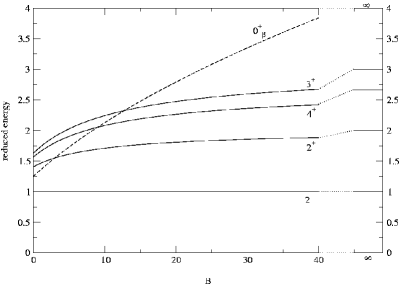
Figure 25: Reduced energies of the lowest state of the $\beta-$band (dashed line) and of a few lowest states of the ground state band (solid lines) as a function of $B$. The limits for the energy levels when $B\rightarrow\infty$, that correspond to the rigid triaxial rotor energies, are reported in the right side. Here we fixed $C=1$.

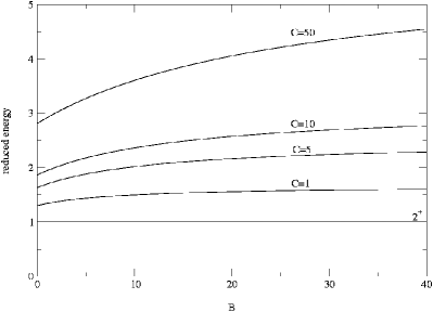
Figure 26: Reduced energies of the ($J^{\pi}=2^{+},n_{\gamma}=1,n_{\beta}=0$) state (solid line) as a function of $B$, for various values of the strength of the harmonic potential in $\gamma$, $C$. The first $2^{+}$ of the ground state band (dashed line) is reported for reference.

We display in fig. 25 and 26 (see captions, adapted from FL ) the behaviour of some energy levels with respect to the parameters of the potential. The Davydov (rigid) model is recovered when $B\rightarrow\infty$ as can be seen from fig. 25.

V.5 Bonatsos’ at al. solution or Z(5)

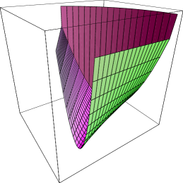
Figure 27: Plot $V(\beta,\gamma)$ of the potential used the so-called Z(5) solution discussed by Bonatsos and collaborators (BonZ5 ): a harmonic oscillator in $\gamma$ with a minimum in $\gamma_{0}=\pi/6$ combined with a square well potential in $\beta$ (the lowest corner of the frame box corresponds to the origin of polar coordinates).

A critical point symmetry for a shape phase transition from prolate ($\gamma=0^{o}$) to oblate ($\gamma=60^{o}$) shapes was introduced in BonZ5 and called Z(5). The authors argue that in such a transition the triaxial region is crossed and the middle lies at $\gamma=30^{o}$. Unless the previous solution the present one does not use an exact separation of variables, but rather an approximate one with $u(\beta,\gamma)=u(\beta)+v(\gamma)$, where the $\beta$ potential is taken to be a square well and the $\gamma$ potential is taken as a harmonic oscillator with the minimum in $\gamma=30^{o}$. The infinite potential well in $\beta$ may be thought as the critical point between a triaxial vibrator (with the minimum close to $\beta=0$) and a triaxial rotator with a minimum for a non null value of $\beta$. In this aspect the model closely resembles the X(5) model.

The same trick adopted in the previous section (formula (128)) is used here to treat the rotational degrees of freedom. The Schrödinger equation is approximatively separated into the set

$$\Bigl{[}-{1\over\beta^{4}}{\partial\over\partial\beta}\beta^{4}{\partial\over\partial\beta}+{1\over 4\beta^{4}}(4L(L+1)-3R^{2})+u(\beta)\Bigr{]}\xi_{L,R}(\beta)=\epsilon_{\beta}\xi_{L,R}(\beta)$$ (136)

and

$$\Bigl{[}-{1\over\langle\beta^{2}\rangle\sin{3\gamma}}{\partial\over\partial\gamma}\sin{3\gamma}{\partial\over\partial\gamma}+u(\gamma)\Bigr{]}\eta(\gamma)=\epsilon_{\gamma}\eta(\gamma)\,,$$ (137)

where the angular momentum quantum number, $L$, and its projection on the intrinsic y-axis, $R$, are explicitely contained in the first equation. In the second equation the average of $\beta^{2}$ over $\xi(\beta)$ appears: this approximation is strictly valid only when the potential $u(\beta)$ is deep and consequently the mean square value of $\beta$ does not oscillate much and remains constant also for a few lower excited states. The energy is $\epsilon\simeq\epsilon_{\beta}+\epsilon_{\gamma}$. With the transformation $\tilde{\xi}(\beta)=\beta^{3/2}\xi(\beta)$ and the substitutions $\epsilon_{\beta}=k_{\beta}^{2}$ and $z=\beta k_{\beta}$, eq. (136) becomes a Bessel equation with eigenfunctions:

$$\xi_{s,\nu}(\beta)=c_{s,\nu}\beta^{-3/2}J_{\nu}(k_{s,\nu}\beta)\,,$$ (138)

where the non-integer index is

$$\nu={\sqrt{4L(L+1)-3R^{2}+9}\over 2}\,.$$ (139)

The boundary condition at the wall of the potential well, $\xi(\beta_{w})=0$, determines the spectrum as a function of $x_{s,\nu}$, the sth zero of the Bessel function $J_{\nu}(z)$

$$\epsilon_{\beta;s,\nu}=\Bigl{(}{x_{s,\nu}\over\beta}\Bigr{)}\,.$$ (140)

The $\gamma-$part is obtained, limiting ourselves to small oscillations around the minimum, from the solution of the equation

$$\Bigl{[}-{\partial^{2}\over\partial x^{2}}+{1\over 2}c\langle\beta^{2}\rangle x^{2}\Bigr{]}\eta(x)=\epsilon_{\gamma}\langle\beta^{2}\rangle\eta(x)\,,$$ (141)

where $\gamma=\pi/6+x$. The above equation is an harmonic oscillator equation with eigenvalues

$$\epsilon_{\gamma}=\sqrt{{2c\over\langle\beta^{2}\rangle}}(n_{\gamma}+1/2)\,,$$ (142)

with $n_{\gamma}=0,1,2,...~{}~{}$. The eigenfunctions are expressed in terms of Hermite polynomials

$$\eta_{n_{\gamma}}(x)=\sqrt{b\over\sqrt{\pi}2^{n_{\gamma}}n_{\gamma}!}H_{n_{\gamma}}(bx)e^{-b^{2}x^{2}/2}$$ (143)

with $b=(c\langle\beta^{2}\rangle/2)^{1/4}$. The index of the Hermite polynomials is now the number of $\gamma-$phonons.

V.6 Jolos’ solution

One of the main objectives of ref. Jolos is to summarize the various researches on shape phase transitions in nuclei. Using the interacting boson model and the coherent state formalism the author analyzes the phase diagram of a cold nucleus discussing the order of phase transitions. Within the same perspective the author summarizes also some of the recent achievements in the solution of the Bohr hamiltonian. In particular he proposes an approximate solution for the critical point of the phase transition between spherical and triaxially deformed shapes. A potential of the form

$$V(\beta,\gamma)=u(\beta)+{1\over 2}D\beta^{6}\cos{(3\gamma)}^{2}$$ (144)

is used. Assuming $D$ large enough, one can consider only small oscillations around $\gamma=\pi/6$, and defining $x=\gamma-\pi/6$, the equation becomes

$$\Biggl{\{}-{\hbar^{2}\over 2B_{m}}\Biggl{[}{1\over\beta^{4}}{\partial\over\partial\beta}\beta^{4}{\partial\over\partial\beta}+{1\over\beta^{2}}\Bigl{(}{\partial^{2}\over\partial x^{2}}-{9DB_{m}\over\hbar^{2}}\beta^{8}x^{2}-L(L+1)+{3\over 4}R^{2}\Bigr{)}+u(\beta)-E\Biggr{\}}\Psi(\beta,\gamma,\theta_{i})=0\,,$$ (145)

where $R$ is once again the projection of $\hat{\vec{L}}$ on the intrinsic y-axis. If the wave function is factorized in the following way

$$\Psi(\beta,\gamma,\theta_{i})=f(\beta)e^{-{B_{m}\omega\over 2\hbar}\beta^{4}x^{2}}{1\over\sqrt{2^{n}n!\sqrt{\pi}}}H_{n}\Bigl{(}x\beta^{2}\sqrt{B_{m}\omega\over\hbar}\Bigr{)}{\cal D}^{L}_{M,R}(\theta_{i})\,,$$ (146)

where $\omega=2(D/B_{m})^{1/2}$ and $H_{n}$ are Hermite polynomials, (having used the original notation), one can exploit the action of the rotational and differential operators in the variable $x$. The equation for the $\beta-$part of the problem is therefore

$$\Biggl{\{}-{\hbar^{2}\over 2B_{m}}\Biggl{[}{1\over\beta^{4}}{\partial\over\partial\beta}\beta^{4}{\partial\over\partial\beta}-{1\over\beta^{2}}\Bigl{(}L(L+1)+{3\over 4}R^{2}\Bigr{)}\Biggr{]}+u(\beta)+\hbar\omega(n+{1\over 2})-E\Biggr{\}}f(\beta)=0\,,$$ (147)

where one can use the infinite square well model for the potential $u(\beta)$ and take the assumption $\beta^{2}\rightarrow\langle\beta^{2}\rangle$. Hence the wavefunction for the $\beta$ part may be written as

$$f(\beta)=\beta^{-3/2}c^{i}_{L,R}J_{\nu}(k^{i}_{L,R}\beta)\,,$$ (148)

where (notice the slight change of notation with respect to the original)

$$\nu=\sqrt{L(L+1)-{3\over 4}R^{2}+{9\over 4}}$$ (149)

and

$$k^{i}_{L,R}=x^{i}_{L,R}/\beta_{w}\,,$$ (150)

with $\beta_{w}$ is the position of the infinite wall and $x^{i}_{L,R}$ is the $i-$th zero, $i=1,2,3,...$ of $J_{\nu}$. Here $c^{i}_{L,R}=\sqrt{2}/\beta_{w}J^{\prime}_{\nu}(x^{i}_{L,R})$. The energy is

$$E^{i}_{L,R}={\hbar^{2}\over 2B_{m}\beta_{w}^{2}}(x^{i}_{L,R})^{2}+\hbar\omega n\langle iLRn\mid\beta^{2}\mid iLRn\rangle.$$ (151)

VI Algebraic methods

We have preferred to dedicate a separate section to the solutions of the Bohr hamiltonian obtained through group theoretical techniques, even if this breaks the chronological order and necessarily implies a redoubling of some topics, because of the insight that they provide. We focus here especially on the results obtained with the su(1,1) algebra. More informations on this argument may be found in refs. Wyb , ch. 18 and cizpa ; CWood , while a thorough group theoretical analysis of the collective model is found in ref. Kem ; MO1 : the works of Chacón, Moshinsky and Sharp and of Kemmer, Pursey and Williams are very often considered as ’classics’ on the group theory of the collective model. Recently Rowe, Turner and Repka RTR gave an useful algorithm for the computation of SO(5) spherical harmonics.

VI.1 Rowe and Bahri’s work

An alternative solution of the harmonic oscillator and of the Davidson potential has been given in ref. Rowe1 . It is easy to recognize that the generalized coordinates of the nuclear collective model, ${q_{\nu}}$ and their conjugate momenta ${\pi_{\nu}}$, may be used to form operators that are closed under commutation. Having defined the scalars products $\beta^{2}~{}=~{}\sum_{\nu}\mid q_{\nu}\mid^{2}$ and $\pi^{2}~{}=~{}\sum_{\nu}\mid\pi_{\nu}\mid^{2}$ we can introduce the operators

$${\hat{Z}}_{1}=\pi^{2}\qquad{\hat{Z}}_{2}~{}=~{}\beta^{2}\qquad{\hat{Z}}_{3}={1\over 2}\sum_{\nu}(q_{\nu}\cdot\pi_{\nu}+\pi_{\nu}\cdot q_{\nu})$$ (152)

that span an $sp(1,{\mathbb{R}})\sim su(1,1)$ algebra. They are in fact closed under commutation:

$$[\hat{Z}_{1},\hat{Z}_{2}]=-4i\hat{Z}_{3}\quad[\hat{Z}_{3},\hat{Z}_{2}]=-2i\hat{Z}_{2}\quad[\hat{Z}_{3},\hat{Z}_{1}]=2i\hat{Z}_{1}\,.$$ (153)

With the linear transformation

$$\hat{X}_{1}~{}=~{}{1\over 4}\bigl{(}\hat{Z}_{1}-\hat{Z}_{2}\bigr{)}\qquad~{}\hat{X}_{2}~{}=~{}{1\over 2}\hat{Z}_{3}\qquad~{}\hat{X}_{3}~{}=~{}{1\over 4}\bigl{(}\hat{Z}_{1}+\hat{Z}_{2}\bigr{)}$$ (154)

one may recognize the standard $su(1,1)\sim so(2,1)$ commutation relations

$$[\hat{X}_{1},\hat{X}_{2}]=-i\hat{X}_{3}\qquad~{}[\hat{X}_{2},\hat{X}_{3}]=i\hat{X}_{1}\qquad~{}[\hat{X}_{3},\hat{X}_{1}]=i\hat{X}_{2}\,.$$ (155)

It is also very useful to the define raising, lowering and weight operators for this algebra (the so-called eigenoperator decomposition)

$$\hat{X}_{\pm}=\hat{X}_{1}\pm i\hat{X}_{2}\qquad\hat{X}_{0}=\hat{X}_{3}$$ (156)

that obey the following commutation relations

$$[\hat{X}_{+},\hat{X}_{-}]=-2\hat{X}_{0}\qquad[\hat{X}_{0},\hat{X}_{\pm}]=\pm\hat{X}_{\pm}\,.$$ (157)

The action of the above operators on orthonormal bases states for the irreps of $su(1,1)$ ($\mid n,\lambda\rangle$ with n=0,1,2,..) is given by the equations:

$$\hat{X}_{+} \mid n\lambda\rangle=\sqrt{(\lambda+n)(n+1)}\mid n+1,\lambda\rangle$$

$$\hat{X}_{-} \mid n+1,\lambda\rangle=\sqrt{(\lambda+n)(n+1)}\mid n\lambda\rangle$$

$$\hat{X}_{0} \mid n\lambda\rangle={1\over 2}(\lambda+2n)\mid n\lambda\rangle~{}~{}~{}~{}~{}~{}~{}~{}~{}~{}~{}~{}~{}~{}~{}$$

The Casimir operator is

$${\hat{\mathbb{C}}}~{}=~{}{\hat{X}}_{3}^{2}-{\hat{X}}_{1}^{2}-{\hat{X}}_{2}^{2}~{}=~{}{\hat{X}}_{0}({\hat{X}}_{0}-1)-{\hat{X}}_{+}{\hat{X}}_{-}~{}=~{}$$

$${1\over 8}\Bigl{(}\hat{Z}_{1}\hat{Z}_{2}+\hat{Z}_{2}\hat{Z}_{1}\Bigr{)}-{\hat{Z}_{3}^{2}\over 4}$$ (159)

and takes the values

$${\hat{\mathbb{C}}}\mid n\lambda\rangle={1\over 4}\lambda(\lambda-2)\mid n\lambda\rangle\,.$$ (160)

From what we have summarized here it follows that the harmonic oscillator hamiltonian may be written as (where we are omitting some $\hbar\omega$ factor)

$${\hat{Z}}_{1}+{\hat{Z}}_{2}~{}=~{}4{\hat{X}}_{3}$$ (161)

which is diagonal in the basis given above. Its spectrum is

$$E_{n\lambda}~{}=~{}(2n+\lambda)$$ (162)

where $\lambda=v+5/2$. With the remarkable nonlinear transformation Rowe1 ; Rowe2

$${\hat{Z}}_{1}\rightarrow{\hat{Z}}_{1}+{\hbar^{2}\epsilon\over{\hat{Z}}_{2}}\qquad{\hat{Z}}_{2}\rightarrow{\hat{Z}}_{2}\qquad{\hat{Z}}_{3}\rightarrow{\hat{Z}}_{3}$$ (163)

the new operators satisfy again the $sp(1,{\mathbb{R}})\sim su(1,1)$ commutation relations. The spectrum

$$E_{nv}~{}=~{}(2n+1+\sqrt{(v+3/2)^{2}+\epsilon})$$ (164)

is found introducing the definition of $\lambda$ that comes from the comparison between the eigenvalues of $\mathbb{C}$ obtained from (160) and (159).

VI.2 Algebraic approach to Coulomb-like and Kratzer-like potentials

The preceeding treatment of the Davidson potential, together with ch. 18 in ref. Wyb , has served as a source of inspiration for the treatment given in FV2 . The spectrum of the Coulomb-like and Kratzer-like potentials may be derived in a similar fashion by noticing that the following operators

$$\hat{Z}_{1}~{}=~{}4\beta\Bigl{(}\pi^{2}+{B\over\beta^{2}}\Bigr{)}\qquad~{}\hat{Z}_{2}~{}=~{}\beta\qquad~{}\hat{Z}_{3}~{}=~{}2\bigl{(}\hat{\vec{q}}\cdot\hat{\vec{\pi}}-i\bigr{)}$$ (165)

are closed under commutation with the same relations of (153). With the Kratzer-like potential (that contains also the Coulomb-like case, when $B=0$) the operator $\beta{\cal H}$ is in fact expressible as a linear combination of the elements of the algebra of $su(1,1)$, namely in the form

$$\beta{\cal H}~{}=~{}\hat{Z}_{1}/4-A.$$ (166)

By defining again raising, lowering and weight operators we can write the eigenvalue equation for the Bohr hamiltonian as

$$\Bigl{[}(1+4\epsilon)\hat{X}_{1}-2A+(1-4\epsilon)\hat{X}_{3}\Bigr{]}\Psi~{}=~{}0$$ (167)

and following the procedure in Ald we can perform a (1,3) hyperbolic rotation of an angle $\theta$ to diagonalize the eigenvalue equation. By choosing $tgh(\theta)=-(1+4\epsilon)/(1-4\epsilon)$ (valid for $\epsilon<0$) we obtain a diagonal relation:

$$\hat{X}_{3}\tilde{\Psi}~{}=~{}{A\over\sqrt{-4\epsilon}}\tilde{\Psi}\,,$$ (168)

where $\tilde{\Psi}$ is the rotated wavefunction. The Casimir operator of the so(2,1) algebra is evaluated to be:

$$\hat{\mathbb{C}}_{2}~{}=~{}\hat{\Lambda}^{2}+\hat{X}_{-}-\hat{X}_{+}+B+2\,,$$ (169)

with eigenvalue $\tau(\tau+3)+B+2$. The two last equations must be compared with the two following eigenvalue equations (for unitary representations $D^{+}$ Baru ):

$$\hat{X}_{3}\mid\phi,\xi\rangle ~{}=~{} (\xi-\phi)\mid\phi,\xi\rangle$$

$$\hat{\mathbb{C}}_{2}\mid\phi,\xi\rangle ~{}=~{} \phi(\phi+1)\mid\phi,\xi\rangle\,.$$ (170)

This comparison yields a spectrum of the form:

$$\epsilon_{\tau,\xi}~{}=~{}-{A^{2}/4\over(\sqrt{(\tau+3/2)^{2}+B}+1/2+\xi)^{2}}$$ (171)

that coincides with the one found from the direct solution of the differential equation with a Kratzer-like potential.

The algebra associated with the SO(5) group plays the role of a degeneracy algebra Cord , while the group SO(2,1) is associated with the spectrum generating algebra. For what concern either the problem considered here and the one in the previous subsection the chain of subalgebras that gives the labels of the set of orthonormal states $\{\mid\xi\tau\alpha LM\rangle\}$ is given as Rowe1 ; Rowe2 ; FV1 :

$$\begin{array}[]{ccccccccc}SU(1,1)&\times&SO(5)&\supset&U(1)&\times&SO(3)&\supset&SO(2)\\ \lambda&{}\hfil&\tau&\alpha&\xi&{}\hfil&L&{}\hfil&M\\ \end{array}$$ (172)

where $\lambda$ is an SU(1,1) lowest weight and $\alpha$ indexes the SO(3) multiplicity. These basis diagonalize the above problems. We can thus state that the problem studied so far displays a SO(2,1)$\times$SO(5) dynamical algebra.

VI.3 Quasidynamical SO(2) symmetry for triaxial nuclei

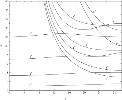
Figure 28: Rotational part of the spectrum of the rigid triaxial rotor (Davydov’s model).

In fig. 28 we plot the eigenvalue of the rigid triaxial rotor hamiltonian (see sect. V) as a function of $\gamma_{0}$. For $\gamma=0$ and $\gamma=\pi/3$ the projection of the third component of the angular momentum on the intrinsic axis 3 gives a good quantum number ($K$), while for $\gamma=\pi/6$ the eigenvalue of the projection on the intrinsic axis 1 is a good quantum number ($R$). In the intermediate regions, none of them may be taken as a good quantum number. Moving from $\gamma=30^{o}$ towards $\gamma=0^{o}$, different groups of states may be classified into bands: a first band ($0^{+},2^{+},4^{+},...$) tend to the finite axial rotor values; a second band ($2^{+},3^{+},4^{+},...$) is identified by its behaviour when $\gamma\rightarrow 0$ (in fig. 28 this group of states somewhat cluster around $\gamma\sim 10^{o}-12^{o}$); the beginning of a third band ($4^{+},5^{+},....$) is seen to escape to infinity at a quicker pace (exiting fig. 28 at around $\gamma\sim 20^{o}$). The experimental observation that a classification in $\beta$ and $\gamma$ bands seems an almost universal feature of nuclear spectra reinforces this choice. The labeling with the $K$ quantum number is often encountered in the literature, although for what we have said here it is not adequate. One may describe this situation in terms of a quasidynamical symmetry RoL ; RoWi of a somewhat strange character: at $\gamma=0^{o}$ the group SO(2) is a symmetry of the system, associated with $K$, while at $\gamma=30^{o}$ another SO(2) group is a symmetry of the system, associated with $R$, being the chain U(5)$\supset$SO(3) common to the whole sector $0\leq\gamma\leq\pi/6$. In the intermediate region $0<\gamma<\pi/6$ the SO(2) symmetry is broken (badly broken in a ’classical’ sense), but it must be noticed (see fig. 28) that the structure of the rotational spectrum present at $\gamma=0^{o}$ persists in the whole sector without being altered in a dramatic way. Only a smooth and slight change may be seen. On the other side the structure of the ’maximally’ triaxial rotor at $\gamma=30^{o}$ persists also in the region around $\gamma\sim 20^{o}-30^{o}$. In the intermediate region these groups of states escape to infinity, as already said. It must be further noticed that the regions where the various states that comes from the axial rotor side are more affected is exactly the region where the states coming from the $\gamma=30^{o}$ triaxial rotor diverge. The strange character of this quasidynamical symmetry mentioned above is that (at variance with the case discussed by Rowe and collaborators RoL ; RoWi , where a true phase transition was present between two exactly solvable limits associated with different symmetries and different group structures) here we are dealing with a smooth transition between two limits which formally have the same underlying group structure, SO(2), and there is no critical point in between. Therefore we conclude that the use of a label that mimics the $K$ quantum number, that retain the formal division in $\beta$ and $\gamma$ bands typical of an axial rotor, is not only justified by the empirical observation that non-axial nuclei display the same classification in bands, but it is also supported in view of arguments based on a group theoretical approach. It is not clear at present if a quantization procedure around a tilted axis may help to further shed light on this aspect.

It is understood, however, that $K$ has been introduced as a convenient label (for basis states and eigenvalues) that comes into play in the branching rules from SO(5) to SO(3) Kem ; RTR .

VII Recent developments of the collective model

We cannot completely neglect, although we will just touch the argument briefly, that the collective model has recently experienced new important developments that are connected with the various solutions that we have summarized in the present review or that furnish new strategies to get numerical solutions. These developments have in common the Streben to simplification and tractability.

VII.1 Caprio’s simplified approach to the CM

The more general hamiltonian of the geometric collective model contains a series expansion in terms in the surface deformation coordinates and their conjugate momenta. The Bohr hamiltonian corresponds to the truncation of all the kinetic terms with order higher than the second. Caprio studied a simplified version Mark2 of the hamiltonian in which only the leading order kinetic term and the three lowest leading order potential terms are retained, namely:

$$H={1\over B_{2}}[\pi\times\pi]^{(0)}+{C_{2}\over\sqrt{5}}\beta^{2}-\sqrt{2\over 35}C_{3}\beta^{3}\cos{3\gamma}+{C_{4}\over 5}\beta^{4}\,.$$ (173)

This hamiltonian has a structure rich enough to encompass rotational, vibrational and $\gamma-$unstable cases, but it’s still very complex and contains four parameters. Caprio exploited analytic scaling relations to reduce the number of parameters from four to two and summarized the predictions of the model on two-dimensional contour plots. He used two ’simple’ observations to make the reduction. Firstly, an overall multiplication of the hamiltonian by a constant does not affect eigenvalues and wave functions. Secondly, with the transformation

$$V(\beta,\gamma)\rightarrow V^{\prime}(\beta,\gamma)=a^{2}V(a\beta,\gamma)$$ (174)

all the eigenvalues are multiplied by $a^{2}$ and the wave functions are radially dilated by $1/a$. Other simplifications and graphs are given in the text to which we refer the reader Mark2 for a more detailed discussion. The author mentions also the difficulty in numerical diagonalization of the problem in the basis of the five-dimensional harmonic oscillator, emphasizing that a large number of basis functions must be used in order to have correct results. A possible solution to this problem is outlined in the following section.

VII.2 Rowe’s tractable version of the CM

The Bohr-Mottelson collective model may in principle be solved numerically for any potential that is an analytic functions of the two variables, but the expansion of rotational wave functions in a spherical vibrational basis is very slowly convergent. The diagonalization is therefore very difficult. Rowe proposed a method in which the basis is constructed with analytic wave functions whose $\beta-$part are centered around a non-zero value Rowe-new . The convergence with this method is much faster for a wide variety of model hamiltonians and this method represents an important improvement over older models. This approach, that we will only briefly sketch, is formulated in an algebraic way using the group SU(1,1)$\times$SO(5) as a dynamical group and recognizing that SO(5)- invariant hamiltonians are diagonalizable using SU(1,1) as a spectrum generating algebra (see Rowe-new for details). The dynamical subgroup chain employed is SU(1,1)$\times$SO(5)$\subset$ SO(5)$\subset$ SO(3). The Davidson potential Dav ; Elli ; Elli2 ; Rowe1 , that is an exactly solvable case, is employed for what concern the dependence on $\beta$. Its exact wave functions are (approximately) centered around the minimum of the potential well and give a good starting point for diagonalization. This simple version may be applied directly to all the cases which lie between the spherical vibrator and the Wilets and Jean ($\gamma-$flat) limit.

A more general extension of use of the basis obtained from the solution of the Bohr hamiltonian with the Davidson potential is also treated. A periodic potential in gamma $V(\gamma)=-\chi\cos{3\gamma}$ is added to the hamiltonian. The reader is referred to the original paper for the details and the discussion. This model is very flexible because of the rich variety of spectra that may generate and it is more physical because of the relaxation of the hypothesis of rigidity. Furthermore it allows for a tractable diagonalization procedure.

In principle this model, with suitable choice of potentials and parameters, should be able to cover the whole complexity of nuclear collective features associated with the quadrupole degree of freedom.

VII.3 Rigid triaxial model with independent inertia moments

In the rigid triaxial rotor model irrotational flow moments of inertia have been usually assumed. In Ref. Wood the rigid triaxial rotor model is studied including the three components of the moments of inertia as parameters that may be fitted to experimental data. The rigid rotor hamiltonian is

$$H~{}=~{}\sum_{i=1}^{3}A_{i}\hat{Q}_{i}^{2}\,,$$ (175)

where the three parameters $A_{i}$ are defined as

$$A_{i}={1\over 2{\cal I}_{i}},\qquad i=1,2,3$$ (176)

and ${\cal I}_{1}\geq{\cal I}_{2}\geq{\cal I}_{3}$. The operators $\hat{Q}_{i}$ are the components of the angular momentum in the body-fixed frame of reference. The hamiltonian (175) may be rewritten in terms of diagonal and non-diagonal operators (using the definitions $\hat{Q}_{\pm}=\hat{Q}_{1}\pm i\hat{Q}_{2}$) as

$$H~{}=~{}A\hat{Q}^{2}+F\hat{Q}_{3}+G(\hat{Q}_{+}^{2}+\hat{Q}_{-}^{2})$$ (177)

where $A=(A_{1}+A_{2})/2$, $F=A_{3}-A$ and $G=(A_{1}-A_{2})/4$. A few low-lying eigenstates may obtained analytically from the diagonalization of the hamiltonian in the rigid rotational basis $\mid LMK\rangle$ and they are summarized in Table 6.

$L$	$E(L)$
0	0
2	$6A+2F\pm 2\sqrt{F^{2}+12G^{2}}$
3	$12A+4F$

Table 6: Low-lying eigenstates of the model described in Wood . Their total angular momentum is also indicated. A few other cases might be solved.

Some of the eigenvectors and electric quadrupole properties are also discussed in the paper and from an analysis it emerges that the components of the moment of inertia are not irrotational. For further discussion we refer the reader to the cited work.

VIII Acknowledgments and apology

I wish to thank M.Caprio (Yale), K.Heyde (Gent) and A.Vitturi (Padova) for their help, encouragement and collaboration and to D.J.Rowe (Toronto) for his kind and keen interest in my work. I also thank G.Lévai (Debrecen) and R.F.Casten (Yale) for the comments on a preliminary draft of this work. Discussions with D.Bonatsos (Tessaloniki), F.Iachello (Yale) and N.Pietralla (SUNY) are also acknowledged. Financial support and warm hospitality are acknowledged from the institutions wherein various parts or stages of this work has been carried on: FWO-Vlaanderen and Universiteit Gent (Belgium), Università di Padova and INFN (Italy) and Universidad de Sevilla (Spain).

We apologize once again with all the researchers whose works have been omitted, mistreated or simply forgotten in the present paper, noticing again that the main purpose was a discussion of solutions of the Bohr hamiltonian. To help the inquisitive reader and to render justice as far as we can we included at the end of the bibliography an additional disordered list of interesting papers whose work for various reasons has not been summarized here f1 ; g ; g1 ; g2 ; g3 ; g4 ; g6 ; g7 ; g8 .

APPENDIX A

Number of repetitions

Within a given set of quantum numbers (a given $\tau$ in the general $\gamma-$unstable case, or $N$ in the harmonic oscillator case) the same $L$ may appear more than once. We define the repetitions of $L$ as the number of counts of that $L$ minus one. Despite the fact that this appendix could seem a purely academic divertissement, its novel number theoretical content is not completely detached from its physical significance: if a model predicts two states that are degenerate in energy to have the same $L$ quantum number it may be very difficult to experimentally disentangle the two. The procedure of assignation of quantum numbers to measured spectra is not free from its own uncertainties and the outcome is a crucial test for theories. It seems thus very important to have a detailed knowledge of what we should expect from our theoretical calculation to look through the data. It will be clear that, in the following cases, the occurrence of repetitions is rather rare and it appears frequently only for high lying states so that likely is not prejudicial to any analysis that was carried on so far.

General $\gamma-$unstable case

We will begin with the general $\gamma-$unstable case: the problem is to count how many repeated multiplicity of SO(3) appears within a given irrep of SO(5), or to count the repetitions of $L$’s for a given $\tau$. Looking at table I in the text we can see that up to $\tau=5$ every $L$ appears just one time, so the number of repetitions is 0. For $\tau=6$, the quantum number $L=6$ appears two times, so the number of repetitions is 1. Continuing along this line one easily finds (by hand in the first few cases) that the number of repetitions, starting from $\tau=6$ is:

$$1,1,2,4,5,7,10,12,15,19,22,26,31,35,40,...$$ (A . 1)

This sequence has been calculated with a simple computer code and it corresponds to the sequence obtained from

$$R(\tau)=\left\{\begin{array}[]{lr}1+\Bigl{[}{n(n-3)\over 6}\Bigr{]}&\tau\geq 6\\ 0&\tau<6\end{array}\right.$$ (A . 2)

with $n=\tau-3=3,4,5,...$, where square brackets denote the integer part, or floor function. Within the same range of $n$ this is also connected to the number of solutions to the equation $x+y+z=0~{}(~{}mod~{}n~{})$ with $0\leq x<y<z<n$. For instance if $n=3$ the only possible solution is $x=0$, $y=1$ and $z=2$. This sequence arises also in connection with the so-called ’orchard problem’ (See Slo ).

Harmonic oscillator case

For the case of harmonic oscillator a further analysis may be done. For a given $N$ a certain number of pairs of $(n_{\beta},\tau)$ satisfy $N=2n_{\beta}+\tau$. For each pair a value of $\tau$ is associated with a set of quantum numbers $L$ (the same of the preceding section). Hence the set of $L$’s corresponding to each $N$ is larger that in the former case (the degree of degeneration is higher) and the sequence of numbers of repetitions, starting from $N=4$, may be written as follows

$$2,3,7,11,18,26,36,48,63,79,99,121,146,...$$ (A . 3)

while in all the cases with $N\leq 3$ there are no repetitions as can be seen from Table II. Unlike the previous case it was not possible to make a connection between the present sequence and any previously known sequence Fors , nor it was possible to find a simple formula to express the $N$th term of the sequence. Note that the number of repetitions in this case is not simply given by

$${\bar{R}}(N)=\sum_{n_{\beta}=0}^{[N/2]}R(\tau=N-2n_{\beta})$$ (A . 4)

because it happens that many repetitions come from different $(n_{\beta},\tau)$ pairs (otherwise they would have started from $N=6$). It is furthermore intriguing to notice that when the terms of the sequence (A . 3) are subtracted with the corresponding terms of the sequence that may be built from formula (A . 4), the remaining sequence (starting from $N=4$) is

$$2,3,6,10,15,21,28,36,45,55,66,....$$ (A . 5)

and apart from the first two elements the differences between two of any other couple of adjacent terms increases arithmetically (!).

Two very simple computer codes, IRREP and IRHAR, written in Fortran77, are available from the author or from WWW sito . They count the number of times that a given quantum number occurs, and give thus the number of repetitions as in (A . 1) and (A . 3) .

APPENDIX B

Meaning of the terms ”softness” and ”rigidity”

The purpose of the present Appendix is to clarify the meaning that should be attributed to the words “softness” and “rigidity” in the context of the collective model.

In general the solution of the Schrödinger equation depends on the potential that is chosen. In the case of the Bohr hamiltonian (restricted to the quadrupole degree of freedom) the potential is a function of $0\leq\beta$ and $0\leq\gamma\leq\pi/3$. Every couple of values ${\beta,\gamma}$ univocally corresponds to a given quadrupole surface. The state of the quantum system is represented by wavefunctions that have a dependence on $\beta$, $\gamma$ or both. When the potential is very deep and narrow its wavefunctions (especially the more low-lying ones) are very localized in the region of the minimum and they may be associated with just one value of $\beta$. The object (that lives in the configuration space) that is described by such state has therefore a rigid shape in the sense that its surface doesn’t exhibit fluctuations. On the contrary a more shallow potential gives rise to extended wavefunctions. This means that the real object may be thought as a superposition of different quadrupole surfaces each with its own weight. The term ”soft” was used to describe such an object. This system exhibits non-null fluctuations around the mean square deformation.

Sometimes it is argued by analogy with the work of Wilets and Jean Wilet that the independence of the potential on one variable is associated with the term softness. The dependence or independence on a given variable should not be used to establish the softness or rigidity of some state. The unstable case of Wilets and Jean (for what concern the $\gamma$ d.o.f., that is a sort of angular variable and not a radial variable) is, among the many possible soft cases, the most extreme one.

For example we may decide to set the potential in $\beta$ to a constant on its whole semi-infinite domain.

In this $\beta-$independent case the eigenstates lie in the continuum and the eigenfunctions have a periodic behaviour at infinity. It is thus not possible to associate a finite value to the deformation of such a state! The situation in the paper of Wilets and Jean is different: two cases were discussed, the infinite square well and the displaced harmonic oscillator. They are both examples of a soft behaviour, because the two quantum mechanical potentials give rise to solutions endowed with extended wavefunctions. One can see that while the displaced oscillator has a true dependence on $\beta$, the infinite square well has a dependence hidden in the boundary conditions (that are essential to fix the spectrum). The analogy with the $\gamma-$unstable case is thus rather feeble, because a $\beta-$unstable counterpart has not a definite physical meaning. The word ”unstable” refers to the fact that the potential has no minima (and hence there’s no ”stability” in the classical sense) and should be read as a synonymous of ”independent”.

In summary the word ”soft” applies to the usual quantum mechanical case, while the word ”rigid” must be associated with very peculiar cases for which either the value of $\beta$ (and/or $\gamma$) is fixed or the potential is of a very special kind. At the beginning of the study of the Bohr-Mottelson model many ”rigid” cases were discussed, mainly for the need of simplicity and for the lack of more refined (”soft”) solutions.

APPENDIX C

Electromagnetic transitions

In some of the spectra displayed in the paper, electromagnetic transition rates have appeared. Although it is not the subject of the present monograph, it is useful to discuss to some extent how they may be derived, especially because BE(2) values, being very sensitive to the details of the wave functions, are often considered as crucial quantities for the application of the aforementioned models to nuclei.

The electromagnetic operator that is often encountered in this context reads:

$$T(E2)=t\beta\Bigl{[}D_{\mu,0}^{(2)}\cos{\gamma}+{1\over\sqrt{2}}(D_{\mu,2}^{(2)}+D_{\mu,-2}^{(2)})\sin{\gamma}\Bigr{]}$$ (C . 1)

where $t$ is a scale factor. This is the first order approximation of the more general E2 operator GG ; EG . In the geometric collective model this operator is written in the laboratory frame coordinates as an expansion:

$$T(E2;\mu)=a\alpha_{2,\mu}+b[\alpha\times\alpha]^{(2)}_{\mu}+{\cal{O}}(\alpha^{3})\,,$$ (C . 2)

where each term is coupled to a total angular momentum equal to 2. It has been often argued Pep ; Capslo that a second order approximation

$$T(E2)=a\beta\Bigl{[}D_{\mu,0}^{(2)}\cos{\gamma}+{1\over\sqrt{2}}(D_{\mu,2}^{(2)}+D_{\mu,-2}^{(2)})\sin{\gamma}\Bigr{]}-b\sqrt{2\over 7}\beta^{2}\Bigl{[}D_{\mu,0}^{(2)}\cos{2\gamma}-{1\over\sqrt{2}}(D_{\mu,2}^{(2)}+D_{\mu,-2}^{(2)})\sin{2\gamma}\Bigr{]}$$ (C . 3)

leads to non-trivial modifications in the calculations of the matrix elements. Transition rates are then calculated in the following way:

$$B(E\lambda;J_{i}\rightarrow J_{f})={\langle J_{i}\mid T(E\lambda)\mid J_{f}\rangle\over 2J_{i}+1}$$ (C . 4)

where $\lambda$ is the angular momentum that characterizes the transition. Usually B(E2) values have been normalized taking the value of the B(E2) for the transition $2_{1}^{+}\rightarrow 0_{1}^{+}$ as 100.

Finally we mention that, for E0 transition, the electromagnetic operator is

$$T(E0)\propto\beta^{2}\,.$$ (C . 5)

References

- (1) Aage Bohr, Dan. Mat. Fys. Medd. 26, no.14 (1952).
- (2) Aage Bohr and Ben Mottelson, Dan. Mat. Fys. Medd. 27, no.16 (1953).
-
(3)
D.M.Brink, Prog.Nucl.Phys. 8, 99 (1960);
D.J.Rowe, Nuclear Collective Motion: Models and Theory, Methuen, London,(1970);
M.A.Preston and R.K.Badhuri, Structure of the nucleus, Addison-Wesley, New York, (1975), ch. 9 ;
R.F.Casten, Nuclear Structure from a Simple Perspective, Oxford University Press, (2000). - (4) J.M.Eisenberg and W.Greiner, Nuclear Models, 3rd ed., vol. 1, North-Holland Physics Pub., Amsterdam, (1987);
- (5) R.V.Jolos, Fiz.Elem.Chast.Atom.Yadra 35 (2004) 408 [or alternatively Phys.Part.Nucl. 35 (2004) 225].
- (6) F.Iachello, Phys.Rev.Lett. 85, 3580 (2000).
- (7) F.Iachello, Phys.Rev.Lett. 87, 052502 (2001).
- (8) B.R.Mottelson, Nobel Lecture (1975).
- (9) N.Bohr and J.Wheeler, Phys.Rev. 56, 426 (1939).
- (10) M.Jean, Nucl.Phys. 21, 142-156 (1960).
- (11) L.Wilets and M.Jean, Phys.Rev. 102, 788 (1956).
- (12) D.Bés, Nucl.Phys. 10, 373-385 (1959).
- (13) T.M.Corrigan et al., Phys.Rev. C14, 2279 (1976).
- (14) P.M.Davidson, Proc.R.Soc. 135, 459 (1932).
- (15) J.P.Elliott et al., Phys.Lett. 169B, 309 (1986).
- (16) J.P.Elliott, P.Park and J.A.Evans, Phys.Lett. B171, 145-147, (1986).
- (17) D.J.Rowe and C.Bahri, J.Phys.A:Math.Gen. 31, 4947 (1998).
- (18) M.A.Caprio, Phys.Rev. C65, 031304(R) (2003)
- (19) L.Fortunato and A.Vitturi, J.Phys.G:Nucl.Part.Phys. 29 1341-1349 (2003)
- (20) A.Erdélyi et al., Higher Transcendental functions, Vol. I, McGraw-Hill book Company, Inc. (1955).
- (21) G.Lévai and J.M.Arias, Phys.Rev. C69, 014304 (2004).
- (22) M.A.Caprio, private communication (Aug. 2003).
- (23) M.A.Caprio, Phys.Rev. C69, 044307 (2004)
- (24) J.N.Ginocchio, Nucl.Phys. A376, 438 (1982)
- (25) J.N.Ginocchio, in Interacting Bose-Fermi Systems in Nuclei, Ed. by F.Iachello - Ettore Majorana International Science Series - Vol. 10 , Series Ed. A.Zichichi (1981).
- (26) S.G.Rohoziński, J.Srebrny and K.Horbaczewska, Z.Physik A 268, 401-408 (1974)
- (27) J.Dobaczewski, S.G.Rohoziński and J.Srebrny, Z.Physik A 282, 203-206 (1977)
- (28) S.T.Belyaev, Nucl.Phys. 64, 17 (1965); K.Kumar and M.Baranger, Nucl.Phys. A92, 608 (1967).
- (29) J.M.Arias, C.E.Alonso, A.Vitturi, J.E.Garcia-Ramos, J.Dukelsky and A.Frank, Phys.Rev. C68 041302 (2003).
- (30) D.Bonatsos, D.Lenis, N.Minkov, P.P.Raychev, P.A.Terziev, Phys.Rev. C69, 014302 (2004).
- (31) D.Bonatsos, D.Lenis, N.Minkov, P.P.Raychev, P.A.Terziev, Phys.Rev. C69, 044316 (2004).
- (32) M.A.Caprio, Phys.Rev. C69, 044307 (2004).
- (33) L.Fortunato and A.Vitturi, J.Phys.G:Nucl.Part.Phys. 30 627 - 635 (2004)
- (34) N.Pietralla and O.M.Gorbachenko, Phys.Rev. C70, 011304(R) (2004).
- (35) D.J.Rowe, private communication (Apr. 2004).
- (36) A.S.Davydov and G.F.Filippov, Nucl.Phys. 8, 237 (1959).
- (37) A.S.Davydov and V.S.Rostovsky, Nucl.Phys. 12, 58-68 (1959).
- (38) A.S.Davydov and A.A.Chaban, Nucl.Phys. 20, 499-508 (1960).
- (39) A.S.Davydov, Nucl.Phys. 24, 682-694 (1961).
- (40) J.Meyer-ter-vehn, Nucl.Phys. A249, 111-140 (1975).
- (41) F.Iachello, Phys.Rev.Lett. 91, 132502 (2003).
- (42) L.Fortunato, Phys.Rev. C70, 011302(R) (2004).
- (43) D.Bonatsos et al., Phys.Lett. B 588, 172-179 (2004).
- (44) B.G.Wybourne, Classical Groups for Physicists, J.Wiley & Sons (1974).
- (45) J.Čízek and J.Paldus, Int.J.Quant.Chem. XII, 875 (1977).
- (46) T.H.Cooke and J.L.Wood, Am.J.Phys. 70, 945 (2002).
- (47) N.Kemmer, D.L.Pursey and S.A.Williams, J.Math.Phys. 9, No.8, 1224-1230 (1968); S.A.Williams and D.L.Pursey, J.Math.Phys. 9, No.8, 1230-1240 (1968);
- (48) E.Chacón, M.Moshinsky and R.T.Sharp, J.Math.Phys. 17, No. 5, 668-676 (1976); E.Chacón and M.Moshinsky, J.Math.Phys. 18, No.5, 870-880 (1977)
- (49) D.J.Rowe, P.S.Turner and J.Repka, J.Math.Phys, 45, 2761 (2004).
- (50) R.Aldrovandi and P.Leal Ferreira, Lett.Nuovo Cimento 1, 317 (1969).
- (51) A.O.Barut and Y.Kitagawara, J.Phys. A:Math. Gen. 14, 2581 (1981).
- (52) P.Cordero and G.C.Ghirardi, Nuovo Cimento 2A, 217 (1971).
- (53) D.J.Rowe, Prog.Part.Nucl.Phys. 37, 265 (1996).
- (54) D.J.Rowe, Phys.Rev.Lett. 93, 122502 (2004).
- (55) D.J.Rowe, C.Bahri and W.Wijesundera, Phys.Rev.Lett. 80, 4394 (1998); C.Bahri, D.J.Rowe and W.Wijesundera, Phys.Rev.C 58, 1539 (1998).
- (56) M.A.Caprio, Phys.Rev. C68 054303 (2003).
- (57) D.J.Rowe, Nucl.Phys. A735, 372-392 (2004).
- (58) J.L.Wood et al., Phys.Rev. C70 024308 (2004).
-
(59)
N.J.A.Sloane, sequence number A058212,
in On-line Encyclopedia of Integer Sequences
by N.J.A.Sloane.
URL: http://www.research.att.com/njas/sequences/ - (60) L.Fortunato, sequence number A090666, in On-line Encyclopedia of Integer Sequences by N.J.A.Sloane.
- (61) L.Fortunato, IRREP and IRHAR codes, URL: http://www.pd.infn.it/fortunat/
- (62) J.M.Arias, Phys.Rev. C63, 034308 (2001).
-
(63)
G.Gneuss and W.Greiner, Nucl.Phys. A171, 449-479 (1971).
———————————————————————– - (64) G.G.Dussel and D.R.Bés, Nucl.Phys. A143, 623-640 (1970).
- (65) A.Gheorghe, A.A.Raduta and V.Ceausescu, Nucl.Phys. A296, 228-250 (1978).
- (66) J.Meyer-ter-Vehn, Phys.Lett. B84, 10-12 (1979).
- (67) M.Moshinsky, Nucl.Phys. A338, 156-166 (1980).
- (68) I.Hamamoto, Prog.Theor.Phys. (Suppl.) 74&75, 157-169 (1983).
- (69) C.Yannouleas and J.M.Pacheco, Comp.Phys.Comm. 54 315-328 (1988)
- (70) Sh. Sharipov and M.J.Ermatov, Int.J.Mod.Phys. E 12, iss. 1, 41-58 (2003).
- (71) Sh. Sharipov and M.J.Ermatov, Int.J.Mod.Phys. E 12, iss. 5, 683-698 (2003).
- (72) R.Bijker et al., Phys.Rev. C68, 064304 (2003); Erratum-ibid. C69, 059901 (2004).