Nucleon Polarisabilities from Compton Scattering
off the One- and Few-Nucleon System

Abstract

These proceedings sketch how combining recent theoretical advances with data from the new generation of high-precision Compton scattering experiments on both the proton and few-nucleon systems offers fresh, detailed insight into the Physics of the nucleon polarisabilities. A multipole-analysis is presented to simplify their interpretation. Predictions from Chiral Effective Field Theory with special emphasis on the spin-polarisabilities can serve as guideline for doubly-polarised experiments below $300$ MeV. The strong energy-dependence of the scalar magnetic dipole-polarisability $\beta_{M1}$ turns out to be crucial to understand the proton and deuteron data. Finally, a high-accuracy determination of the proton and neutron polarisabilities shows that they are identical within error-bars. For details and a better list of references, consult Refs. [1, 2, 3, 4].

1 Introduction

Nuclear physicists are hardly surprised by the fact that the nucleon is not a point-like spin-$\frac{1}{2}$ target with an anomalous magnetic moment in low-energy Compton scattering $\gamma N\to\gamma N$. Rather, the photon field displaces its charged constituents, inducing a non-vanishing multipole-moment. These nucleon-structure effects have in fact been known for many decades and (in the case of a proton target) quite reliable theoretical calculations for the deviations from the Powell cross-section exist. They are canonically parameterised starting from the most general interaction between the nucleon $N$ with spin $\vec{\sigma}/2$ and an electro-magnetic field of fixed, non-zero energy $\omega$:

$$\begin{split}&2\pi\;N^{\dagger}\;\big{[}\alpha_{E1}(\omega)\;\vec{E}^{2}\;+\;\beta_{M1}(\omega)\;\vec{B}^{2}\;+\;\gamma_{E1E1}(\omega)\;\vec{\sigma}\cdot(\vec{E}\times\dot{\vec{E}})\;+\;\gamma_{M1M1}(\omega)\;\vec{\sigma}\cdot(\vec{B}\times\dot{\vec{B}})\\ &\;\;\;\;\;\;\;\;\;\;\;\;-\;2\gamma_{M1E2}(\omega)\;\sigma_{i}\;B_{j}\;E_{ij}\;+\;2\gamma_{E1M2}(\omega)\;\sigma_{i}\;E_{j}\;B_{ij}\;+\;\dots\big{]}\;N\end{split}$$ (1)

Here, the electric or magnetic ($X,Y=E,M$) photon undergoes a transition $Xl\to Yl^{\prime}$ of definite multipolarity $l,l^{\prime}=l\pm\{0,1\}$; $T_{ij}:=\frac{1}{2}(\partial_{i}T_{j}+\partial_{j}T_{i})$, and the coefficients are the energy-dependent or dynamical polarisabilities of the nucleon. Most prominently, there are six dipole-polarisabilities: two spin-independent ones ($\alpha_{E1}(\omega)$, $\beta_{M1}(\omega)$) for electric and magnetic dipole-transitions which do not couple to the nucleon-spin; and in the spin-sector, two diagonal (“pure”) spin-polarisabilities ($\gamma_{E1E1}(\omega)$, $\gamma_{M1M1}(\omega)$) and two off-diagonal (“mixed”) spin-polarisabilities, $\gamma_{E1M2}(\omega)$ and $\gamma_{M1E2}(\omega)$. In addition, there are negligible contributions from higher ones like quadrupole polarisabilities, see Sect. 3.

Polarisabilities measure hence the global stiffness of the nucleon’s internal degrees of freedom against displacement in an electric or magnetic field of definite multipolarity and non-vanishing frequency $\omega$. They contain detailed information about the constituents because they lead to quite different dispersive effects: There are low-lying nuclear resonances like the $\Delta(1232)$, the charged meson-cloud around the nucleon, internal relaxation effects, etc. Spin-polarisabilities are particularly interesting as they parameterise the response of the nucleon-spin to the photon field, having no classical analogon.

It must be stressed that dynamical polarisabilities are a concept complementary to generalised polarisabilities. The latter probe the nucleon in virtual Compton scattering, i.e. with an incoming photon of zero energy and non-zero virtuality, and can provide information about the spatial distribution of charge and magnetism inside the nucleon. Dynamical polarisabilities on the other hand test the global response of the internal nucleonic degrees of freedom to a real photon of non-zero energy and answer the question which internal degrees of freedom govern the structure of the nucleon at low energies by parameterising the time-scale on which the interaction takes place.

Nucleon Compton scattering provides thus a wealth of information about the internal structure of the nucleon. However, in contradistinction to many other electro-magnetic processes, the nucleon-structure effects probed in Compton scattering have not been analysed in terms of a multipole-expansion at fixed energies. Instead, most experiments have focused on just two parameters, namely the static electric and magnetic polarisabilities $\bar{\alpha}:=\alpha_{E1}(\omega=0)$ and $\bar{\beta}:=\beta_{M1}(\omega=0)$, which are also often for brevity called “the polarisabilities” of the nucleon. Therefore, quite different theoretical frameworks are at present able to provide a consistent, qualitative picture for the leading static polarisabilities. Their dynamical origin is however only properly revealed by their energy-dependence, which varies with the underlying mechanism. For the proton, the generally accepted static values are $\bar{\alpha}^{p}\approx 12\times 10^{-4}\;\mathrm{fm}^{3},\;\bar{\beta}^{p}\approx 2\times 10^{-4}\;\mathrm{fm}^{3}$, with error-bars of about $1\times 10^{-4}\;\mathrm{fm}^{3}$. For the neutron, different types of experiments report a range of values $\bar{\alpha}^{n}\in[-4;19]$, and even less is known about the spin-polarisabilities.

These notes give an overview how combining recent theoretical advances with data from the new generation of high-precision Compton scattering experiments also with polarised beams and targets can offer fresh, detailed insight into these problems: We define dynamical polarisabilities and study their low-energy contents in Sect. 2, together with a model-independent extraction of the scalar dipole-polarisabilities of the proton. Section 3 proposes to extract their energy-dependence and simultaneously determine the ill-known spin-polarisabilities by polarised experiments. Finally, an accurate determination of the neutron polarisabilities from deuteron Compton scattering is reported in Sect. 4.

2 Definition and Low-Energy Contents

A rigorous definition of energy-dependent or dynamical polarisabilities starts instead of (LABEL:polsfromints) from the six independent amplitudes into which the $T$-matrix of real Compton scattering is decomposed:

$$T(\omega,z) = A_{1}(\omega,z)\;(\vec{\epsilon}\,^{\prime*}\cdot\vec{\epsilon})+A_{2}(\omega,z)\;(\vec{\epsilon}\,^{\prime*}\cdot\hat{\vec{k}})\;(\vec{\epsilon}\cdot\hat{\vec{k}}^{\prime})+\mathrm{i}\,A_{3}(\omega,z)\;\vec{\sigma}\cdot\left(\vec{\epsilon}\,^{\prime*}\times\vec{\epsilon}\,\right)$$

$$+\mathrm{i}\,A_{4}(\omega,z)\;\vec{\sigma}\cdot\left(\hat{\vec{k}}^{\prime}\times\hat{\vec{k}}\right)(\vec{\epsilon}\,^{\prime*}\cdot\vec{\epsilon})+\mathrm{i}\,A_{5}(\omega,z)\;\vec{\sigma}\cdot\left[\left(\vec{\epsilon}\,^{\prime*}\times\hat{\vec{k}}\right)\,(\vec{\epsilon}\cdot\hat{\vec{k}}^{\prime})-\left(\vec{\epsilon}\times\hat{\vec{k}}^{\prime}\right)\,(\vec{\epsilon}\,^{\prime*}\cdot\hat{\vec{k}})\right]$$

$$+\mathrm{i}\,A_{6}(\omega,z)\;\vec{\sigma}\cdot\left[\left(\vec{\epsilon}\,^{\prime*}\times\hat{\vec{k}}^{\prime}\right)\,(\vec{\epsilon}\cdot\hat{\vec{k}}^{\prime})-\left(\vec{\epsilon}\times\hat{\vec{k}}\right)\,(\vec{\epsilon}\,^{\prime*}\cdot\hat{\vec{k}})\right]$$

Here, $\hat{\vec{k}}$ ($\hat{\vec{k}}^{\prime}$) is the unit-vector in the momentum direction of the incoming (outgoing) photon with polarisation $\vec{\epsilon}$ ($\vec{\epsilon}\,^{\prime*}$) and $\theta$ the scattering angle, $z=\cos\theta$.

We separate these amplitudes into a pole-part and a non-pole or structure-part $\bar{A}_{i}$. Intuitively, one could define the pole-part as the one which leads to the Powell cross-section of a point-like nucleon with anomalous magnetic moment and thus parameterises all we hope to have understood about the nucleon. Then, it would seem, the structure-part contains all information about the internal degrees of freedom which make the nucleon an extended, polarisable object. However, the question which part a contribution belongs to cannot be answered uniquely. In the following, only those terms which have a pole either in the $s$-, $u$- or $t$-channel are treated as non-structure, see Ref. [2] for details. This means for example that the large contribution to the spin-polarisabilities from the $\pi^{0}\gamma\gamma$-vertex via a $\pi^{0}$-pole in the $t$-channel is not part of the polarisabilities thus defined. In the calculation of observables, such a separation is clearly irrelevant because the structure-dependent and structure-independent part must be summed. Here, however, we investigate the rôle of the internal nucleonic degrees of freedom for the polarisabilities. They are contained only in the structure-part of the amplitudes.

We also choose to work in the centre-of-mass frame. Thus, $\omega$ denotes the cm-energy of the photon, $M$ the nucleon mass, and $W=\sqrt{s}$ the total cm-energy. Following older work on the multipole-decomposition of the Compton amplitudes and pulling a kinematical factor out relative to (LABEL:polsfromints), one obtains for the expansion of the structure-parts of the amplitudes in terms of polarisabilities

$$\bar{A}_{1}(\omega,\,z) \displaystyle=\frac{4\pi\,W}{M}\,\left[\alpha_{E1}(\omega)+z\,\beta_{M1}(\omega)\right]\,\omega^{2}+\dots,\;\;\;\;\bar{A}_{2}(\omega,\,z)\displaystyle=-\frac{4\pi\,W}{M}\,\beta_{M1}(\omega)\,\omega^{2}+\dots,$$

$$\bar{A}_{3}(\omega,\,z) \displaystyle=-\frac{4\pi\,W}{M}\,\left[\gamma_{E1E1}(\omega)+z\,\gamma_{M1M1}(\omega)+\gamma_{E1M2}(\omega)+z\,\gamma_{M1E2}(\omega)\right]\,\omega^{3}+\dots,$$

$$\bar{A}_{4}(\omega,\,z) \displaystyle=\frac{4\pi\,W}{M}\,\left[-\gamma_{M1M1}(\omega)+\gamma_{M1E2}(\omega)\right]\,\omega^{3}+\dots,$$ (3)

$$\bar{A}_{5}(\omega,\,z) \displaystyle=\frac{4\pi\,W}{M}\,\gamma_{M1M1}(\omega)\,\omega^{3}+\dots,\;\;\;\;\bar{A}_{6}(\omega,\,z)=\frac{4\pi\,W}{M}\,\gamma_{E1M2}(\omega)\,\omega^{3}+\dots$$

The various polarisabilities are thus identified at fixed energy only by their different angular dependence. Clearly, the complete set of dynamical polarisabilities does – like all quantities defined by multipole-decompositions – not contain more or less information about the temporal response or dispersive effects of the nucleonic degrees of freedom than the un-truncated Compton amplitudes. However, the information is more readily accessible and easier to interpret: Each mechanism and channel leaves a characteristic signature in the polarisabilities. Moreover, it will turn out that all polarisabilities beyond the dipole ones can be dropped in (3), as they are so far invisible in observables. For that reason, they were sacrificed to brevity in the expressions above and purists should consider Ref. [2].

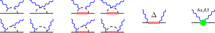
To identify the microscopically dominant low-energy degrees of freedom inside the nucleon in a model-independent way, we employ the unique low-energy theory of QCD, namely Chiral Effective Field Theory ($\chi$EFT). This extension of Chiral Perturbation Theory to the few-nucleon sector contains only those low-energy degrees of freedom which are observed at the typical energy of the process, interacting in all ways allowed by the underlying symmetries of QCD. A power-counting allows for results of finite, systematically improvable accuracy and thus for an error-estimate. The resulting contributions at leading order, listed in Fig. 1, are easily motivated:

• Photons couple to the charged pion cloud around the nucleon and around the $\Delta$, signalled by a characteristic cusp at the one-pion production threshold.

• It is well-known that the $\Delta(1232)$ as the lowest nuclear resonance can be excited in the intermediate state by the strong $\gamma N\Delta$ $M1$-transition, leading to a para-magnetic contribution to the static magnetic dipole-polarisability $\bar{\beta}_{\Delta}=+[7\dots 13]$. Its signal is a characteristic resonance-shape, as in the Lorentz model of polarisabilities in classical electro-dynamics.

• As the observed static value $\bar{\beta}^{p}\approx 2$ is smaller by a factor of $5$ than the $\Delta$ contribution, a strongly dia-magnetic component must exist. The resultant fine-tuning at zero photon-energy is unlikely to hold once the evolution of the polarisabilities with the photon energy is considered: If dia- and para-magnetism are of different origin, it is more than likely that they involve different scales and hence different energy-dependences. Therefore, they are apt to be dis-entangled by dynamical polarisabilities. We sub-sume this short-distance Physics which is at this order not generated by the pion or $\Delta$ into two energy-independent low-energy coefficients $\delta\alpha,\;\delta\beta$. While naïve dimensional analysis sees them suppressed by an order of magnitude, $|\delta\alpha|\sim|\delta\beta|\approx\frac{\alpha}{\Lambda_{\chi}^{2}M}\sim 1$ with $\Lambda_{\chi}\approx 1$ GeV the breakdown-scale of $\chi$EFT, the facts require them to be included at leading order already.

Figure 1: The dominant interactions in $\chi$EFT which give rise to the nucleon polarisabilities. Left to right: pion cloud around the nucleon and $\Delta$; $\Delta$ excitations; short-distance effects. Permutations and crossed diagrams not shown. From Ref. [2].

Figure 2: Typical differential cross-sections for proton Compton scattering. Left: Data and $\chi$EFT without polarisabilities (dash-dotted); with only dipole-polarisabilities (dashed); full amplitude (dotted). Right: Dispersion Theory (solid) compared to $\chi$EFT with (long dashed) and without $\Delta$ contributions ($\mathcal{O}(p^{3})$: short dashed; $\mathcal{O}(p^{4})$: dotted). From Refs. [2, 8].

The free constants $\delta\alpha$ and $\delta\beta$ are determined by fitting the un-expanded $\chi$EFT-amplitude to the cornucopia of Compton scattering data on the proton [5, 6] below $200\;\mathrm{MeV}$, cf. Fig. 2. If these values are consistent within error-bars with the Baldin sum-rule for the proton, $\bar{\alpha}^{p}+\bar{\beta}^{p}=13.8\pm 0.4$, one can in a second step use this number as additional input. One obtains indeed

$$\begin{array}[]{rll}\mbox{free fit:}&\displaystyle\bar{\alpha}^{p}=11.5\pm 2.4_{\mathrm{stat}}&,\;\;\;\;\bar{\beta}^{p}=3.4\pm 1.7_{\mathrm{stat}}\\ \mbox{with Baldin:}&\displaystyle\bar{\alpha}^{p}=11.0\pm 1.4_{\mathrm{stat}}\pm 0.4_{\mathrm{Baldin}}&,\;\;\;\;\bar{\beta}^{p}=2.8\mp 1.4_{\mathrm{stat}}\pm 0.4_{\mathrm{Baldin}}\end{array}$$ (4)

Higher-order corrections are estimated to contribute an error of about $\pm 1$ not displayed here. The statistical error dominates. These results compare both in magnitude and uncertainty favourably with state-of-the-art results e.g. from a global data-analysis [5] or from Dispersion Theory [7]:

$$\begin{array}[]{rll}\mbox{dispersion theory:}&\bar{\alpha}^{p}=12.4\pm 0.6_{\mathrm{stat}}\mp 0.6_{\mathrm{syst}}&,\;\;\;\;\bar{\beta}^{p}=1.4\pm 0.7_{\mathrm{stat}}\pm 0.5_{\mathrm{syst}}\end{array}$$ (5)

The two short-distance parameters are indeed anomalously large, $\delta\alpha=-5.9\pm 1.4,\;\delta\beta=-10.7\pm 1.2$, justifying their inclusion at leading order. As expected, $\delta\beta$ is dia-magnetic. Truncating the multipole-expansion in (3) is justified because the influence of the quadrupole and higher polarisabilities on cross-sections and asymmetries for energies up to about $300\;\mathrm{MeV}$ is hardly visible, cf. Figs. 2 and 4.

Not surprisingly, the $\Delta$-contribution is most pronounced at large momentum-transfers, i.e. backward angles, where even the next-to-leading order calculation without dynamical $\Delta$ cannot reproduce the steep rise seen in the data as low as $120\;\mathrm{MeV}$. For that reason, about half of the proton data below $200\;\mathrm{MeV}$ were excluded in the analysis leading to the final numbers in [8].

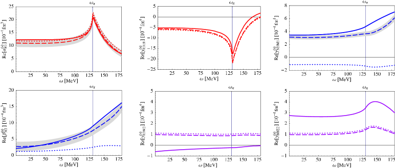
With the parameters now fixed, the energy-dependence of all polarisabilities is predicted. The proton and neutron polarisabilities are very similar in $\chi$EFT, iso-vectorial effects being of higher order. This point will be confirmed also in Sect. 4. We compare with a result from Dispersion Theory, in which the dispersive effects are sub-sumed into integrals over experimental input from a different kinematical régime, namely the photo-absorption cross-section $\gamma N\to X$. Its major error-sources are the insufficient neutron data and the uncertainty in modelling the high-energy behaviour of the dispersive integral.

The dipole-polarisabilities show the expected behaviour, and thus no low-energy degrees of freedom inside the nucleon are missing. Figure 3 shows that dynamical effects are large at photon energies of $80-200\;\mathrm{MeV}$ where most experiments to determine polarisabilities are performed. Especially at large backward angle, unpolarised and polarised cross-sections are rather sensitive to the non-analytical structure of the amplitude around the pion cusp and $\Delta$-resonance, see Figs. 2 and 4, and [2, 3, 4].

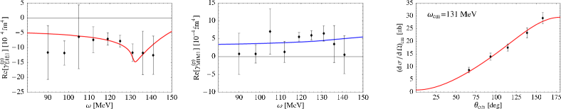
The pion-cusp – clearly seen in the $E1$-polarisabilities – is quantitatively understood already at leading order. The dipole spin-polarisabilities are predictions, three of them being independent of the parameter-determination. Since the mixed spin-polarisabilities (lower centre and right panel of Fig. 3) are small, the relative uncertainties in both Dispersion Theory and $\chi$EFT are large. While the static polarisabilities are real, the dynamical polarisabilities become complex once the energy in the intermediate state is high enough to create an on-shell intermediate state, the first being the physical $\pi N$-continuum, see [2].

Most notably is however the strong energy-dependence induced into $\beta_{M1}(\omega)$ and all polarisabilities containing an $M1$ photon even well below the pion-production threshold by the unique signature of the $\Delta$ resonance: At $\omega\approx 90$ MeV, $\beta_{M1}$ is already about $3$ units larger than its static value, rendering the traditional approximation of $\beta_{M1}(\omega)$ as “static-plus-small-slope” $\bar{\beta}+\omega^{2}\bar{\beta}_{\nu}$ inadequate. This also reveals the good quantitative agreement between the measured value of $\bar{\beta}^{p}$ and the prediction in a $\chi$EFT without explicit $\Delta$ as accidental: The contribution from the pion-cloud alone is not dispersive enough to explain the energy-dependence of $\beta_{M1}$. One could include higher-order terms in the photon-nucleon interactions which mimic the $\Delta$, but their strengthes are then a-priori un-determined. Furthermore, as the effect is strong, this would in-validate the power-counting at the heart of a model-independent analysis. When the $\Delta$ is included, $\gamma_{M1M1}$ even changes sign and $\gamma_{M1E2}$ nearly triples in magnitude. While the fine details of the rising para-magnetism differ between $\chi$EFT and Dispersion Theory, they are consistent within the uncertainties of the $\chi$EFT curve. The discrepancy between the two schemes above the one-pion production threshold is connected to a derailed treatment of the width of the $\Delta$-resonance, which is neglected in leading-one-loop $\chi$EFT at low energies.

Figure 3: The dipole-polarisabilities, predicted by Dispersion Theory (solid) and $\chi$EFT with (dashed, band from fit-errors) and without (dotted) explicit $\Delta$. Left: spin-independent; middle, right: spin-dependent. $\omega_{\pi}$: one-pion production threshold. From Ref. [2].

The two short-distance parameters $\delta\alpha,\;\delta\beta$ which sub-sume all Physics not generated by the pion cloud or the $\Delta$ suffice to describe the polarisabilities up to energies of $300\;\mathrm{MeV}$ when the finite width of the $\Delta$ is included [2]. Therefore, three constraints arise on any attempt to explain them microscopically:

• The effect must be $\omega$-independent over a wide range, like $\delta\alpha,\;\delta\beta$.

• It must occur in the electric and magnetic scalar polarisabilities, leading to the values for $\delta\alpha,\;\delta\beta$ predicted in $\chi$EFT, but it must be absent at least in the pure spin-polarisabilities $\gamma_{E1E1},\;\gamma_{M1M1}$.

• Its prediction for the proton and neutron must be similar because iso-vectorial effects were shown to be small and energy-independent [2, 4], see also the neutron polarisabilities discussed in Sect. 4.

Two proposals to explain $\delta\alpha,\;\delta\beta$ were put forward: One attributes them to an interplay between short-distance Physics and the pion cloud occuring from the next-to-leading order chiral Lagrangean [9]; the other to the $t$-channel exchange of a meson or correlated two-pion exchange [10]. Whether either gives a quantitative description of the short-distance coefficients meeting these criteria is not clear yet.

3 Spin-Polarisabilities and Energy-Dependence from Data

Future doubly-polarised, high-accuracy experiments in particular around the pion-production threshold provide an exciting avenue to extract the energy-dependence of the six polarisabilities per nucleon, both spin-independent [2] and spin-dependent [3]. This is particularly interesting since practically no direct information exists at present on the spin-polarisabilities: Only two linear combinations are constrained from experiments [7], and only at zero photon-energy. These forward and backward spin-polarisabilities $\bar{\gamma}_{0}$ and $\bar{\gamma}_{\pi}$ of the nucleon involve however all four static (dipole) spin-polarisabilities.

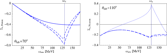
Consider the Compton scattering asymmetry $\Sigma_{x}$: The nucleon-spin lies in the reaction-plane and perpendicular to the circularly polarised incoming photon. Figure 4 shows strong sensitivity on the spin-polarisabilities $\gamma_{i}(\omega)$ and on $\Delta$-Physics, while higher polarisabilities are negligible. Similar findings hold for other asymmetries also with linearly polarised photons [3, 11].

Figure 4: Typical sensitivity of the proton (left) and neutron (right) Compton scattering asymmetry $\Sigma_{x}$. Left, solid lines: no polarisabilities; short dashed: no $\Delta$ Physics; long dashed: full $\chi$EFT. Right, dashed lines: full $\chi$EFT result; dotted: without spin-polarisabilities; dot-dashed: without quadrupole polarisabilities. From Ref. [3].

With higher polarisabilities negligible, one can use the multipole-expansion of the scattering amplitudes (3) to perform with increasing sophistication fits of the six dipole-polarisabilities per nucleon to data-sets which combine polarised and spin-averaged experiments, taken at fixed energy but varying scattering angle [3]. As starting values for the fit, one might assume that the energy-dependence of the polarisabilities derived above in $\chi$EFT is correct, with deviations taken as energy-independent. The corresponding free normalisation for each dipole-polarisability can be used to determine the static values. At low energies, this should be a viable procedure because only $\Delta$- and pion-degrees of freedom are expected to give dispersive contributions to the polarisabilities, and $\chi$EFT predicts their behaviour model-independently. When the fit of eq. (3) to data is made at each energy independently, repeating this procedure for various energies gives the energy-dependence of the polarisabilities. In this way, one can extract dynamical polarisabilities directly from the angular dependence of observables.

The spin-independent polarisabilities $\alpha_{E1}(\omega)$, $\beta_{M1}(\omega)$ from $\chi$EFT in Fig. 3 agree very well with Dispersion Theory, both in their energy-dependence and overall size. They could therefore be used in a second step as input to reduce the number of fit functions in (3) to four, namely the four dipole spin-polarisabilities. The good agreement in $\gamma_{E1E1}(\omega)$ and possibly $\gamma_{M1M1}(\omega)$ can – similarly – be used to reduce the number of fit functions further to three or two per nucleon: $\gamma_{E1M2}(\omega)$ and $\gamma_{M1E2}(\omega)$.

At present, only un-polarised data are available, in which the dipole spin-polarisabilities are however anything but negligible. As a feasibility-study, we demonstrate the method by a superficial fit of the pure spin-polarisabilities to the existing data under the assumption that the mixed spin-polarisabilities are negligible and the spin-independent polarisabilities are predicted correctly [11]. Clearly, today’s un-polarised data are only sensitive to a linear combination of spin-polarisabilities and the error-bars are rather large as the dependence on the spin-polarisabilities is quadratic in $\cos\theta$, while the data are nearly linear at fixed $\omega$, see Fig. 5.

Figure 5: Feasibility study of a multipole-decomposition using existing data. Statistical error-bars only; solid: $\chi$EFT-prediction. From Ref. [11].

To analyse Compton scattering via a multipole-decomposition at fixed energies can thus substantially further our knowledge on the spin-structure of the proton.

4 Neutron Polarisabilities and Deuteron Compton Data

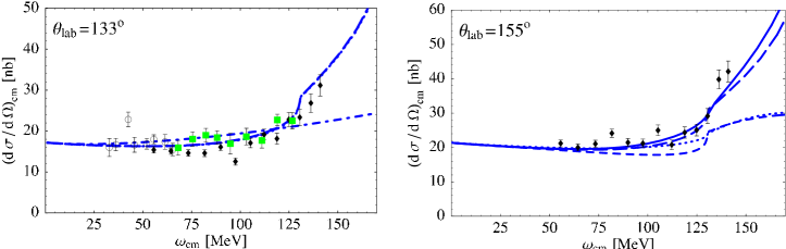
Does the neutron react similarly under deformations, $\bar{\alpha}^{p}\approx\bar{\alpha}^{n}$, $\bar{\beta}^{p}\approx\bar{\beta}^{n}$, etc, as $\chi$EFT predicts? Since free neutrons can only rarely be used in experiments, their properties are usually extracted from data taken on few-nucleon systems by subtracting nuclear-binding effects. This should be done in a model-independent way and with an estimate of the theoretical uncertainties as in $\chi$EFT. However, different types of experiments report a range of values $\bar{\alpha}^{n}\in[-4;19]$: Coulomb scattering of neutrons off lead, or deuteron Compton-scattering with and without breakup, see [4] for a list. As deuteron Compton scattering should provide a clean way to extract the iso-scalar polarisabilities $\bar{\alpha}^{s}:=\frac{1}{2}(\bar{\alpha}^{p}+\bar{\alpha}^{n})$ and $\bar{\beta}^{s}$ parallel to determinations of the proton polarisabilities, experiments were performed [12] in Urbana at $\omega=49$ and $69$ MeV, in Saskatoon (SAL) at $94$ MeV, and in Lund at $55$ and $66$ MeV. While the low-energy extractions are consistent with small iso-vectorial polarisabilities, the SAL data lead to conflicting analyses: The original publication gave $\bar{\alpha}^{s}=8.8\pm 1.0$, employing the Baldin sum-rule for the static nucleon polarisabilities, $\bar{\alpha}^{s}+\bar{\beta}^{s}=14.5\pm 0.6$. Levchuk and L’vov obtained $\bar{\alpha}^{s}=11\pm 2,\;\bar{\beta}^{s}=7\pm 2$ [13]; and Beane et al. found recently from all data $\bar{\alpha}^{s}=13\pm 4,\;\bar{\beta}^{s}=-2\pm 3$ [8]. The extraction being very sensitive to the polarisabilities, can embedding the neutron into a nucleus lead to the discrepancy?

Figure 6: Deuteron Compton scattering in $\chi$EFT to $\mathcal{O}(\epsilon^{3})$. Left: one-body (dots: electric/magnetic couplings; blob: nucleon polarisabilities, Fig. 1). Right: two-body parts (pion-exchange currents). Permutations and crossed diagrams not shown. From Ref. [4].

Figure 7: Deuteron Compton scattering in $\chi$EFT at $\mathcal{O}(\epsilon^{3})$ with $\bar{\alpha}^{s},\;\bar{\beta}^{s}$ from eq. (8), using the Baldin sum rule. Top: Grey bands: Statistical error. Bottom: Comparison between $\chi$EFT with explicit $\Delta$ (solid) and without explicit $\Delta$ (dashed: $\mathcal{O}(p^{3})$, parameter-free; dotted: $\mathcal{O}(p^{4})$, best fit). From Ref. [4] with the help of Ref. [8].

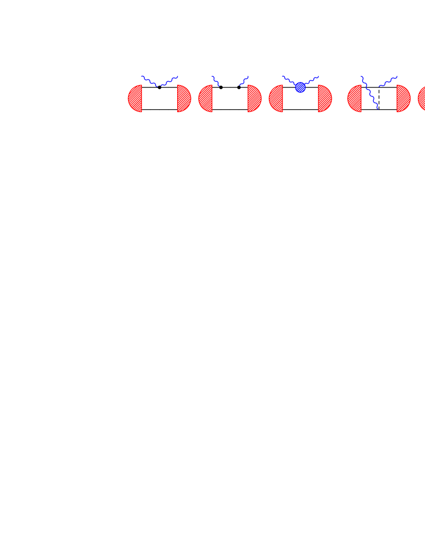
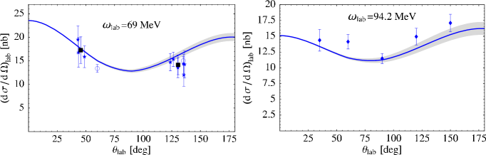
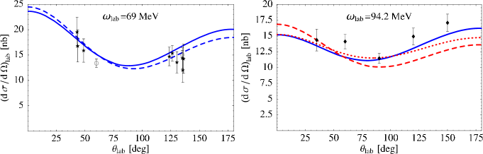
Of course, two-body contributions from meson-exchange currents and wave-function dependence must be subtracted from data with minimal theoretical prejudice. Figure 6 lists the contributions to Compton scattering off the deuteron to next-to-leading order in $\chi$EFT. The calculation is parameter-free, except for the short-distance coefficients $\delta\alpha,\;\delta\beta$ in the nucleon polarisabilities. The nucleon- and nuclear-structure contributions clearly separate at this (and the next) order. While the two-nucleon piece does not contain the $\Delta(1232)$-resonance in the intermediate state at this order as the deuteron is an iso-scalar target, this is not true for the polarisabilities, as seen in Sect 2. Figure 7 shows that the strong energy-dependence from exciting the $\Delta$ is indeed pivotal to reproduce the shape of the data at $94$ MeV in particular at back-angles. Thus, we argue that the discrepancy in extractions from the SAL data and at lower energies is resolved.

So far, dynamical effects had largely been neglected in the analyses: Truncating the Taylor-expansion of the polarisabilities around zero-photon energy at order $\omega^{2}$ under-estimates $\beta_{M1}(\omega=95\;\mathrm{MeV})-\bar{\beta}\approx 1.7$ [13], while our multipole-analysis gives $\approx 4$ (Fig. 3). The $\chi$EFT-calculation of Beane et al. [8] cited already in the proton-extraction uses the same deuteron wave-functions and meson-exchange currents as we, but sub-sume all $\Delta$-effects into short-distance operators which enter only at higher order and are only weakly dispersive. They hence exclude the two SAL-points at large angles from their final analysis.

Fitting in $\chi$EFT with explicit $\Delta$ the two short-distance parameters $\delta\alpha,\;\delta\beta$ to deuteron Compton scattering data above $60$ MeV (Fig. 7), one finds as static values:

$$\begin{array}[]{rll}\mbox{free fit:}&\displaystyle\bar{\alpha}^{s}=12.8\pm 1.4_{\mathrm{stat}}\pm 1.1_{\mathrm{wavefu}}&,\;\;\bar{\beta}^{s}=2.1\pm 1.7_{\mathrm{stat}}\pm 0.1_{\mathrm{wavefu}}\\ \mbox{with Baldin:}&\displaystyle\bar{\alpha}^{s}=12.6\pm 0.8_{\mathrm{stat}}\pm 0.7_{\mathrm{wavefu}}\pm 0.6_{\mathrm{Baldin}}&,\;\;\bar{\beta}^{s}=1.9\mp 0.8_{\mathrm{stat}}\mp 0.7_{\mathrm{wavefu}}\pm 0.6_{\mathrm{Baldin}}\end{array}$$ (8)

Again, higher-order effects can be estimated to induce an additional systematic error of $\pm 1$. The Baldin sum-rule $\bar{\alpha}^{s}+\bar{\beta}^{s}=14.5\pm 0.6$ is already well-reproduced by the unconstrained fit. Comparing with the static proton polarisabilities (4) determined by the same method, the proton and neutron polarisabilities turn indeed out identical within the statistical uncertainty.

5 Perspectives

Dynamical polarisabilities test the global response of the nucleon to the electric and magnetic fields of a real photon with non-zero energy and definite multipolarity. They answer the question which internal degrees of freedom govern the structure of the nucleon at low energies and can be defined by a multipole-expansion of the Compton amplitudes. While they do not contain more or less information than the corresponding Compton scattering amplitudes, the facts are more readily accessible and easier to interpret. Dispersive effects in particular from the $\Delta(1232)$ are necessary to obtain accurate extractions for the static polarisabilities of the nucleon from the available data. Future work includes:

(i) The non-zero width of the $\Delta$ and higher-order effects from the pion-cloud become crucial when probing the nucleon-response in the resonance region.

(ii) As seen, a multipole-analysis from doubly-polarised, high-accuracy experiments provides a new avenue to extract the energy-dependence of the six dipole-polarisabilities per nucleon, both spin-independent and spin-dependent [2, 3, 11]. This will in particular further our knowledge on the spin-polarisabilities, and hence on the spin-structure of the nucleon. A (certainly incomplete) list of planned or approved experiments at photon-energies below $300\;\mathrm{MeV}$ shows the concerted effort in this field: polarised photons on polarised protons, deuterons and ³He at TUNL/HI$\gamma$S; tagged protons at S-DALINAC; polarised photons on polarised protons at MAMI; and deuteron targets at MAXlab. With for example only 29 (un-polarised) points for the deuteron in a small energy range of $\omega\in[49;94]$ MeV and error-bars on the order of $15\%$, new data can improve the situation substantially.

(iii) The deuteron data at $49$ and $55$ MeV [12] are not included in our analysis because the $\chi$EFT-power-counting of Fig. 6 is not tailored to the low-energy end and must be modified to yield the correct Thomson limit. This problem is partially circumvented in Ref. [8], and a full treatment is in its finishing stages [11]. On the other hand, the pion-exchange terms can be integrated out at lower energies, and one arrives at the “pion-less” EFT of QCD. Not only is this version computationally considerably less involved than the pion-ful version $\chi$EFT; it also has the advantage that the Thomson limit is recovered trivially. While Compton scattering becomes the less sensitive to the polarisabilities the lower the energy, a window exists between about $25$ and $50$ MeV where dispersive effects are negligible and this variant can aid high-accuracy experiments e.g. at HI$\gamma$S to extract the static polarisabilities in a model-independent way. Recently, Chen et al. [15] demonstrated that due to the large iso-vectorial magnetic moment, the vector amplitudes in $d\gamma$-scattering are anomalously enhanced in this version. Adding to a previous calculation by Rupak and Grießhammer [14], they found that the data at $49$ and $55$ MeV are in fact well in agreement with the values given above and report $\bar{\alpha}^{s}=12\pm 1.5,\;\bar{\beta}^{s}=5\pm 2$.

Enlightening insight into the electro-magnetic structure of the nucleon has already been gained from combining Compton scattering off nucleons and few-nucleon systems with $\chi$EFT and energy-dependent or dynamical polarisabilities; and a host of activities should add to it in the coming years.

References

- [1] H. W. Grießhammer and T. R. Hemmert: Phys. Rev. C65 (2002), 045207 [nucl-th/0110006].
- [2] R. P. Hildebrandt, H. W. Grießhammer, T. R. Hemmert and B. Pasquini: Eur. Phys. J. A20 (2004), 293 [nucl-th/0307070].
- [3] R. P. Hildebrandt, H. W. Grießhammer and T. R. Hemmert: Eur. Phys. J. A20 (2004), 329 [nucl-th/0308054].
- [4] R.P. Hildebrandt, H.W. Grießhammer, T.R. Hemmert and D.R. Phillips: [nucl-th/0405077]. Accepted for publication in Eur. Phys. J. A.
- [5] Olmos de Leon et al.: Eur. Phys. J. A10 (2001) 207.
- [6] The most recent ones besides Ref. [5] are E.L. Hallin et al., Phys. Rev. C48 (1993) 1497; F.J. Federspiel et al., Phys. Rev. Lett.67 (1991) 1511; B.E. MacGibbon et al., Phys. Rev. C52 (1995) 2097.
- [7] D. Drechsel, B. Pasquini, M. Vanderhaeghen: Phys. Rep. 378 (2003), 99.
- [8] S.R. Beane et al.: [nucl-th/0403088], and private communication.
- [9] V. Bernard et al.: Z. Phys. A348 (1994), 317.
- [10] P. A. M. Guichon, private communication; W. Weise and B. Pasquini: forthcoming.
- [11] R.P. Hildebrandt, H.W. Grießhammer and T.R. Hemmert: forthcoming.
- [12] M.A. Lucas: Ph.D. thesis, Univ. of Illinois at Urbana-Champaign (1994); M. Lundin et al.: Phys. Rev. Lett. 90, 192501 (2003) [nucl-ex/0204014]; D.L. Hornidge et al.: Phys. Rev. Lett. 84 (2000) 2334 [nucl-ex/9909015].
- [13] M. I. Levchuk and A. I. L’vov: Nucl. Phys. A674 (2000) 449 [nucl-th/9909066]; Nucl. Phys. A684 (2001) 490 [nucl-th/0010059].
- [14] H.W. Grießhammer and G. Rupak: Phys. Lett. B529 (2002) 57 [nucl-th/0012096].
- [15] J.W. Chen, X.D. Ji and Y.C. Li: [nucl-th/0408003].