Particle-number conservation
within self-consistent random-phase approximation

Abstract

The self-consistent random-phase approximation (SCRPA) is reexamined within a multilevel-pairing model with double degeneracy. It is shown that the expressions for occupation numbers used in the original version of SCRPA violate the particle number for non-symmetric particle-hole ($ph$) spectra. A renormalization is introduced to restore the particle number, which leads to the expressions of occupation numbers similar to those derived by Hara et al. for the $ph$ case. The results of calculations within the $ph$ symmetric case show that this number-conserving SCRPA yields the energies of the ground state and first excited state of the system with $\Omega+2$ particles relative to the ground state of the system with $\Omega$ particles in close agreement with those obtained within the original SCRPA. However it gives a slightly larger correlation energy.

I Introduction

The random-phase approximation (RPA) has been a powerful tool in the theoretical study of many-body systems such as atomic nuclei. An essential ingredient of the RPA is the use of the quasiboson approximation (QBA), which considers fermion pairs as boson operators, just neglecting the Pauli principle between them. Within the QBA a set of linear equations, which is usually called the RPA equation, is derived, which makes computationally demanding problems become tractable. However, because of the violation of Pauli principle within the QBA, the RPA equation breaks down at a certain critical value of the interaction’s parameter, where the RPA yields imaginary solutions.

Several approaches were developed to remove this inconsistency of the RPA. One of the popular ones is the renormalized RPA (RRPA) Hara (1, 2, 3, 4). The RRPA includes in the expectation value over the ground state the contribution of the diagonal elements of the commutator between two fermion-pair operators. In this way it takes the Pauli principle into account approximately. This includes the so-called ground-state correlations beyond RPA, which eventually renormalize the interaction in such a way that the collapse of RPA is avoided. However, the tests carried out within exactly solvable models also showed that there is still a large discrepancy between the solution obtained within the RRPA and the exact one beyond the RPA collapsing point (See Ref. CaDaSa (4) e.g.).

The situation has been significantly improved recently within the self-consistent RPA (SCRPA) Duk (5, 6, 7) due to the inclusion of screening corrections in the SCRPA equation. These screening corrections are in fact the expectation values of the products of two fermion pairs in the correlated ground state. As the result the sign of the interaction is reversed so that, within a particle-hole ($ph$) symmetric multilevel-pairing model with double degeneracy (the so-called picket-fence model), the SCRPA yields the solutions very close to the exact ones for the correlation energy of the system with $\Omega$ particles, as well as the energy of the first excited state of the system with $\Omega+2$ particles Dukelsky (6, 7).

Realistic nuclear single-particle spectra are in general $ph$ non-symmetric, which means that the particle-particle ($pp$) submatrix $A$ and hole-hole ($hh$) submatrix $C$ of the $pp$-RPA equation do not have the same dimension. The asymmetry is particularly strong, e.g., in light neutron-rich nuclei  VinhMau (8), for which the effect due to Pauli principle cannot be neglected. It is, therefore, worthwhile to reexamine carefully the SCRPA before applying it to realistic nuclei.

The present paper employs the same picket-fence model, which was used to tested the validity of the SCRPA in Refs. Dukelsky (6, 7). It will be shown that, in the general $ph$ non-symmetric case, using its original expressions of ground-state correlation factors, the SCRPA violates the particle number. A simple and consistent way to restore the particle number will be introduced and the consequences will be discussed.

The paper is organized as follows. The outline of the SCRPA for the picket-fence model is presented in Sec. II. The violation of particle number within the SCRPA for $ph$ non-symmetric case and the construction of a number-conserving SCRPA are discussed in Sec. III. The results of numerical calculations are analyzed in Sec. IV. The paper is summarized in the last section, where conclusions are drawn.

II SCRPA equation for the picket-fence model

The detail derivation of self-consistent $pp$ RPA equation, which is simply called SCRPA equation hereafter has been described Refs. Duk (5, 6, 7). The present section recuperates only the brief outline of the SCRPA for the picket-fence model, which is needed for the discussion in this paper.

II.1 Model Hamiltonian

The picket-fence model consists of $\Omega$ two-fold equidistant levels interacting via a pairing force with a constant parameter $G$. The model Hamiltonian is written as

$$H=\sum_{i=1}^{\Omega}(\epsilon_{i}-\lambda)N_{i}-G\sum_{i,j=1}^{\Omega}P_{i}^{\dagger}P_{j}~{},$$ (1)

where the particle-number operator $N_{i}$ and pairing operators $P_{i}^{\dagger}$, $P_{i}$ are given as

$$N_{i}=c_{i}^{\dagger}c_{i}+c_{-i}^{\dagger}c_{-i}~{},\hskip 14.22636ptP_{i}^{\dagger}=c_{i}^{\dagger}c_{-i}^{\dagger}~{},\hskip 14.22636ptP_{i}=(P_{i}^{\dagger})^{\dagger}~{}.$$ (2)

The exact commutation relations between the operators $N_{i}$, $P_{i}^{\dagger}$, and $P_{i}$ are

$$[P_{i},P_{j}^{\dagger}]=\delta_{ij}(1-N_{i})~{},$$ (3)

$$[N_{i},P_{j}^{\dagger}]=2\delta_{ij}P_{j}^{\dagger},~{}\hskip 14.22636pt[N_{i},P_{j}]=-2\delta_{ij}P_{j}~{}.$$ (4)

The single-particle energies take the values $\epsilon_{i}=i\epsilon$ with $i$ running over all $\Omega$ levels. The original version of the SCRPA in Refs. Dukelsky (6, 7) was applied only to a $ph$-symmetric spectrum, where there are as many particles as levels (half filling). This means that, in the absence of interaction ($G=$0), the lowest $\Omega_{h}=\Omega/2$ levels are occupied with $N=\Omega$ particles (two particles in each level). However, in general, the number $\Omega_{h}$ of hole levels is not necessary to be the same as the number $\Omega_{p}$ of particle levels, i.e. $\Omega_{h}\neq\Omega_{p}\neq\Omega/2$. Numerating particle ($p$) and hole ($h$) levels from the levels closest to the Fermi surface, the particle and hole energies are equal to $\epsilon_{p}=\epsilon(\Omega_{h}+p)$ and $\epsilon_{h}=\epsilon(\Omega_{h}-h+1)$, respectively, with $h$ indices running from 1 to $\Omega_{h}$, and $p$ indices running from 1 to $\Omega_{p}=\Omega-\Omega_{h}$. The Fermi level $\lambda$ is defined in the middle of the the first $h$ and the first $p$ levels, i.e.

$$\lambda=\epsilon\big{(}\Omega_{h}+\frac{1}{2}\big{)}-\frac{G}{2}~{}.$$ (5)

Therefore, in the $ph$ symmetric case ($\Omega_{p}=\Omega_{h}=\Omega/2$), the Fermi level $\lambda=[\epsilon(\Omega+1)-G]/2$ is located in the middle of the single-particle spectrum.

Using the notation of Ref. Hirsch (7)

$$M_{p}=N_{p}~{},\hskip 14.22636ptM_{h}=2-N_{h}~{},\hskip 14.22636ptQ^{\dagger}_{p}=P^{\dagger}_{p}~{},\hskip 14.22636ptQ_{h}=-P^{\dagger}_{h}~{},$$ (6)

and also introducing the ground-state correlation operators $D_{p}$ and $D_{h}$

$$D_{p}=1-M_{p}=1-N_{p}~{},\hskip 14.22636ptD_{h}=1-M_{h}=N_{h}-1~{},$$ (7)

the exact commutation relations (3) and (4) can be transformed into

$$[Q_{p},Q_{p^{\prime}}^{\dagger}]=\delta_{pp^{\prime}}D_{p}~{},\hskip 14.22636pt[Q_{h},Q_{h^{\prime}}^{\dagger}]=\delta_{hh^{\prime}}D_{h}~{},$$ (8)

$$[M_{i},Q_{j}^{\dagger}]=2\delta_{ij}Q_{j}^{\dagger}~{},\hskip 14.22636pt[M_{i},Q_{j}]=-2\delta_{ij}Q_{j}~{}.$$ (9)

Using the definition (5) of the Fermi energy $\lambda$ together with notations (6) and (7), Hamiltonian (1) is rewritten in the following form

$$H=-\epsilon\Omega_{h}^{2}+\sum_{p=1}^{\Omega_{p}}\big{[}\epsilon(p-\frac{1}{2})+\frac{G}{2}\big{]}M_{p}+\sum_{h=1}^{\Omega_{h}}\big{[}\epsilon(h-\frac{1}{2})+\frac{G}{2}\big{]}M_{h}$$

$$-G\sum_{pp^{\prime}}Q_{p}^{\dagger}Q_{p^{\prime}}-G\sum_{hh^{\prime}}Q_{h}^{\dagger}Q_{h^{\prime}}+G\sum_{ph}(Q_{p}^{\dagger}Q_{h}^{\dagger}+Q_{p}Q_{h})~{},$$ (10)

which, in the $ph$ symmetric case, coincides with Eq. (13) of Ref. Hirsch (7)  .

II.2 SCRPA equation

The SCRPA equation is derived based on the RRPA additional and removal operators, which have the form

$$A_{\mu}^{\dagger}=\sum_{p}^{\Omega_{p}}{X_{p}^{\mu}}\overline{Q}_{p}^{\dagger}-\sum_{h}^{\Omega_{h}}{Y_{h}^{\mu}}\overline{Q}_{h}~{},$$ (11)

and

$$R_{\lambda}^{\dagger}=\sum_{h}^{\Omega_{h}}{X_{h}^{\lambda}}\overline{Q}_{h}^{\dagger}-\sum_{p}^{\Omega_{p}}Y_{p}^{\lambda}\overline{Q}_{p}~{},$$ (12)

respectively , with the abbreviation

$$\overline{\cal O}_{i}^{\dagger}=\frac{{\cal O}_{i}^{\dagger}}{\sqrt{\langle D_{i}\rangle}}~{},\hskip 14.22636pt\overline{\cal O}_{i}=\frac{{\cal O}_{i}}{\sqrt{\langle D_{i}\rangle}}~{},\hskip 14.22636pti=p,~{}h~{}$$ (13)

to denote the renormalized operator of an operator ${\cal O}_{i}^{\dagger}$. Operator $A_{\mu}^{\dagger}$ transfers the states in a system with $\Omega$ particles to those of a system with $\Omega$+2 particles. Operator $R_{\lambda}^{\dagger}$ transfers the states of an $\Omega$-particle system to those of a system with $\Omega$-2 particles. The brackets $\langle\ldots\rangle\equiv\langle\Omega,0|\ldots|\Omega,0\rangle$ denote the average over the correlated ground state $|\Omega,0\rangle$ of the system with $\Omega$ particles, which is defined as the vacuum of operators $A_{\mu}$ and $R_{\lambda}$, i.e.

$$A_{\mu}|\Omega,0\rangle=R_{\lambda}|\Omega,0\rangle=0~{}.$$ (14)

Using the exact commutation relation (8) and the definition (14) of the RPA ground state $|\Omega,0\rangle$, one can see that the additional and removal operators satisfy the boson commutation relations in the ground state $|\Omega,0\rangle$

$$\langle[A_{\mu},A_{\mu^{\prime}}^{\dagger}]\rangle=\delta_{\mu\mu^{\prime}}~{},\hskip 14.22636pt\langle[R_{\lambda},R_{\lambda^{\prime}}^{\dagger}]\rangle=\delta_{\lambda\lambda^{\prime}}~{},$$ (15)

if the amplitudes $X$ and $Y$ satisfy the following normalization (orthogonality) conditions

$$\sum_{p}X_{p}^{\mu}X_{p}^{\mu^{\prime}}-\sum_{h}Y_{h}^{\mu}Y_{h}^{\mu^{\prime}}=\delta_{\mu\mu^{\prime}}~{},\hskip 5.69054pt\sum_{h}X_{h}^{\lambda}X_{h}^{\lambda^{\prime}}-\sum_{p}Y_{p}^{\lambda}Y_{p}^{\lambda^{\prime}}=\delta_{\lambda\lambda^{\prime}}~{},\hskip 5.69054pt\sum_{p}X_{p}^{\mu}Y_{p}^{\lambda}-\sum_{h}X_{h}^{\lambda}Y_{h}^{\mu}=0~{},$$ (16)

while the closure relations

$$\sum_{\mu}X_{p}^{\mu}X_{p^{\prime}}^{\mu}-\sum_{\lambda}Y_{p}^{\lambda}Y_{p^{\prime}}^{\lambda}=\delta_{pp^{\prime}}~{},\hskip 5.69054pt\sum_{\lambda}X_{h}^{\lambda}X_{h^{\prime}}^{\lambda}-\sum_{\mu}Y_{h}^{\mu}Y_{h^{\prime}}^{\mu}=\delta_{hh^{\prime}}~{},\hskip 5.69054pt\sum_{\lambda}X_{h}^{\lambda}Y_{p}^{\lambda}-\sum_{\mu}X_{p}^{\mu}Y_{h}^{\mu}=0~{}$$ (17)

guarantee the following inverse transformation of Eqs. (11) and (12)

$$Q_{p}^{\dagger}=\sqrt{\langle D_{p}\rangle}\bigg{[}\sum_{\mu}X_{p}^{\mu}A_{\mu}^{\dagger}+\sum_{\lambda}Y_{p}^{\lambda}R_{\lambda}\bigg{]}~{},$$

$$Q_{h}=\sqrt{\langle D_{h}\rangle}\bigg{[}\sum_{\lambda}X_{h}^{\lambda}R_{\lambda}+\sum_{\mu}Y_{h}^{\mu}A_{\mu}^{\dagger}\bigg{]}~{}.$$ (18)

The SCRPA equation is obtained in a standard way by linearizing the equation of motion. The matrix form of the SCRPA equation for the additional mode is

$$\left(\begin{array}[]{cc}{A}&{B}\\ -{B}&{C}\end{array}\right)\left(\begin{array}[]{c}{X^{\mu}}\\ {Y^{\mu}}\end{array}\right)=E_{\mu}\left(\begin{array}[]{c}{X^{\mu}}\\ {Y^{\mu}}\end{array}\right)~{},$$ (19)

where the submatrices $A$, $B$, and $C$ were derived in Ref. Hirsch (7) using the definition (7) as well as the exact commutation relations (8) and (9) as

$$A_{pp^{\prime}}=\langle[~{}\overline{Q}_{p},[H,\overline{Q}_{p^{\prime}}^{\dagger}]]\rangle=$$

$$2\bigg{\{}\big{[}\epsilon(p-\frac{1}{2})+\frac{G}{2}\big{]}+\frac{G}{\langle D_{p}\rangle}\big{[}\sum_{p^{\prime\prime}}\langle Q_{p^{\prime\prime}}^{\dagger}Q_{p}\rangle-\sum_{h^{\prime\prime}}\langle Q_{p}Q_{h^{\prime\prime}}\rangle\big{]}\bigg{\}}\delta_{pp^{\prime}}-G\frac{\langle D_{p}D_{p^{\prime}}\rangle}{\sqrt{\langle D_{p}\rangle\langle D_{p^{\prime}}\rangle}}~{},$$ (20)

$$B_{ph}=-\langle[~{}\overline{Q}_{p},[H,\overline{Q}_{h}]]\rangle=G\frac{\langle D_{p}D_{h}\rangle}{\sqrt{\langle D_{p}\rangle\langle D_{h}\rangle}}~{},$$ (21)

$$C_{hh^{\prime}}=-\langle[~{}\overline{Q}_{h},[H,\overline{Q}_{h^{\prime}}^{\dagger}]]\rangle=$$

$$-2\bigg{\{}\big{[}\epsilon(h-\frac{1}{2})+\frac{G}{2}\big{]}+\frac{G}{\langle D_{h}\rangle}\big{[}\sum_{h^{\prime\prime}}\langle Q_{h}^{\dagger}Q_{h^{\prime\prime}}\rangle-\sum_{p^{\prime\prime}}\langle Q_{p^{\prime\prime}}^{\dagger}Q_{h}^{\dagger}\rangle\big{]}\bigg{\}}\delta_{hh^{\prime}}+G\frac{\langle D_{h}D_{h^{\prime}}\rangle}{\sqrt{\langle D_{h}\rangle\langle D_{h^{\prime}}\rangle}}~{}.$$ (22)

The expectation values of the products of two pair operators at the right-hand side (rhs) of Eqs. (20) and (22) are

$$\langle Q_{p}^{\dagger}Q_{p^{\prime}}\rangle=\langle P_{p}^{\dagger}P_{p^{\prime}}\rangle=\sqrt{\langle D_{p}\rangle\langle D_{p^{\prime}}\rangle}\sum_{\lambda}Y_{p}^{\lambda}Y_{p^{\prime}}^{\lambda}~{},$$ (23)

$$\langle Q_{p}Q_{h}\rangle=\langle Q_{h}^{\dagger}Q_{p}^{\dagger}\rangle=-\langle P_{h}^{\dagger}P_{p}\rangle=-\langle P_{p}^{\dagger}P_{h}\rangle=\sqrt{\langle D_{p}\rangle\langle D_{h}\rangle}\sum_{\lambda}X_{h}^{\lambda}Y_{p}^{\lambda}~{},$$ (24)

$$\langle Q_{h}^{\dagger}Q_{h^{\prime}}\rangle=\sqrt{\langle D_{h}\rangle\langle D_{h^{\prime}}\rangle}\sum_{\mu}Y_{h}^{\mu}Y_{h^{\prime}}^{\mu}=\langle P_{h^{\prime}}^{\dagger}P_{h}\rangle-\delta_{hh^{\prime}}\langle D_{h}\rangle~{},$$ (25)

$${\rm with}\hskip 8.53581pt\langle P_{h^{\prime}}^{\dagger}P_{h}\rangle=\sqrt{\langle D_{h}\rangle\langle D_{h^{\prime}}\rangle}\sum_{\lambda}X_{h}^{\lambda}X_{h^{\prime}}^{\lambda}~{}.$$

They were derived using the inverse transformation (18) and the definition of the ground state (14). The RRPA equation was obtained from Eqs. (19) – (22) by using the factorization

$$\langle D_{i}D_{j}\rangle\simeq\langle D_{i}\rangle\langle D_{j}\rangle~{},$$ (26)

and neglecting all the expectation values $\langle Q^{\dagger}_{p^{\prime}}Q_{p}\rangle$, $\langle Q_{p}Q_{h}\rangle$, and $\langle Q_{h}^{\dagger}Q_{h^{\prime}}\rangle$. The RRPA submatrices have then the form

$$A_{pp^{\prime}}^{\rm RRPA}=2\big{[}\epsilon(p-\frac{1}{2})+\frac{G}{2}\big{]}\delta_{pp^{\prime}}-G\sqrt{\langle D_{p}\rangle\langle D_{p^{\prime}}\rangle}~{},$$ (27)

$$B_{ph}^{\rm RRPA}=G\sqrt{\langle D_{p}\rangle\langle D_{h}\rangle}~{},$$ (28)

$$C_{hh^{\prime}}^{\rm RRPA}=-2\big{[}\epsilon(h-\frac{1}{2})+\frac{G}{2}\big{]}\delta_{hh^{\prime}}+G\sqrt{\langle D_{h}\rangle\langle D_{h^{\prime}}\rangle}~{}.$$ (29)

The RPA submatrices are obtained from the RRPA ones by putting $D_{p}=D_{h}=$ 1, namely

$$A_{pp^{\prime}}^{\rm RPA}=2\big{[}\epsilon(p-\frac{1}{2})+\frac{G}{2}\big{]}\delta_{pp^{\prime}}-G~{},$$ (30)

$$B_{ph}^{\rm RPA}=G~{},$$ (31)

$$C_{hh^{\prime}}^{\rm RPA}=-2\big{[}\epsilon(h-\frac{1}{2})+\frac{G}{2}\big{]}\delta_{hh^{\prime}}+G~{}.$$ (32)

By using definition (6), Eqs. (23) – (25), and recalling that

$$\epsilon_{p}-\lambda=[\epsilon(p-\frac{1}{2})+\frac{G}{2}]~{},$$ (33)

$$\epsilon_{h}-\lambda=-\epsilon(h-\frac{1}{2})+\frac{G}{2}=-[\epsilon(h-\frac{1}{2})+\frac{G}{2}]+G~{},$$ (34)

one can rewrite Eqs. (20) – (22) in the notations of Ref. Dukelsky (6) as

$$A_{pp^{\prime}}=\langle[\overline{P}_{p},[H,\overline{P}_{p^{\prime}}^{\dagger}]]\rangle=2\delta_{pp^{\prime}}(\epsilon_{p^{\prime}}-\lambda)$$

$$+2G\delta_{pp^{\prime}}\frac{\sum_{p^{\prime\prime}}\langle P_{p^{\prime\prime}}^{\dagger}P_{p}\rangle+\sum_{h^{\prime\prime}}\langle P_{h^{\prime\prime}}^{\dagger}P_{p}\rangle}{1-\langle N_{p}\rangle}-G\frac{\langle(1-N_{p})(1-N_{p^{\prime}})\rangle}{\sqrt{(1-\langle N_{p}\rangle)(1-\langle N_{p^{\prime}}\rangle)}}~{},$$ (35)

$$B_{ph}=\langle[\overline{P}_{p},[H,\overline{P}_{h}^{\dagger}]]\rangle=G\frac{\langle(1-N_{p})(N_{h}-1)\rangle}{\sqrt{(1-\langle N_{p}\rangle)(\langle N_{h}\rangle-1)}}~{},$$ (36)

$$C_{hh^{\prime}}=-\langle[\overline{P}_{h},[H,\overline{P}_{h^{\prime}}^{\dagger}]]\rangle=2\delta_{hh^{\prime}}(\epsilon_{h^{\prime}}-\lambda)$$

$$-2G\delta_{hh^{\prime}}\frac{\sum_{h^{\prime\prime}}\langle P_{h^{\prime\prime}}^{\dagger}P_{h}\rangle+\sum_{p^{\prime\prime}}\langle P_{p^{\prime\prime}}^{\dagger}P_{h}\rangle}{\langle N_{h}\rangle-1}+G\frac{\langle(N_{h}-1)(N_{h^{\prime}}-1)\rangle}{\sqrt{(\langle N_{h}\rangle-1)(\langle N_{h^{\prime}}\rangle-1)}}~{}.$$ (37)

II.3 Correlation energy

The correlation energy $E_{\rm corr}^{\rm SCRPA}$ is defined as the difference between the energy ${\cal E}^{\Omega}_{0}\equiv\langle H\rangle$ in the ground state $|\Omega,0\rangle$ (14) and the Hartree-Fock (HF) energy ${\cal E}_{\rm HF}$. The former is easily obtained from Eq. (10) while the later is $-\epsilon\Omega_{h}^{2}$. The final expression for the correlation energy is obtained as

$$E_{\rm corr}^{\rm SCRPA}\equiv\langle H\rangle-{\cal E}_{\rm HF}=\sum_{p}^{\Omega_{p}}\big{[}\epsilon(p-\frac{1}{2})+\frac{G}{2}\big{]}(1-\langle D_{p}\rangle)+\sum_{h}^{\Omega_{h}}\big{[}\epsilon(h-\frac{1}{2})+\frac{G}{2}\big{]}(1-\langle D_{h}\rangle)$$

$$-G[\sum_{pp^{\prime}}\langle Q_{p}^{\dagger}Q_{p^{\prime}}\rangle+\sum_{hh^{\prime}}\langle Q_{h}^{\dagger}Q_{h^{\prime}}\rangle-2\sum_{ph}\langle Q_{p}^{\dagger}Q_{h}^{\dagger}\rangle]~{},$$ (38)

where $\langle Q_{i}^{\dagger}Q_{i}\rangle$ and $\langle Q_{p}^{\dagger}Q_{h}^{\dagger}\rangle$ are given by Eqs. (23) – (25), and $D_{i}$ by Eq. (47).

For comparison, the correlation energy within the RRPA is derived here by approximating the Hamiltonian (1) as

$$H\simeq H^{\rm RRPA}={\cal E}_{0}^{(\Omega)}({\rm RRPA})+\sum_{\mu}E_{\mu}^{\rm RRPA}A_{\mu}^{\dagger}A_{\mu}+\sum_{\lambda}E_{\lambda}^{\rm RRPA}R_{\lambda}^{\dagger}R_{\lambda}~{},$$ (39)

where ${\cal E}^{(\Omega)}_{0}({\rm RRPA})$ is the energy in the RRPA ground state, while the eigenvalues $E_{\mu}^{\rm RRPA}$ and $E_{\lambda}^{\rm RRPA}$ are the excitation energies (42) and (43) of the additional and removal modes, respectively, which are obtained by solving the RRPA equation, i.e. Eq. (19) with submatrices (27) – (29). The correlation energy $E_{\rm corr}^{\rm RRPA}={\cal E}_{0}^{\Omega}({\rm RRPA})-{\cal E}_{\rm HF}$ is obtained by calculating the expectation value of Hamiltonian (39) in the HF ground state $|{\rm HF}\rangle$. By using Eqs. (11) and (12) as well as the definition of $|{\rm HF}\rangle$, for which $P_{p}|{\rm HF}\rangle=\langle{\rm HF}|P_{p}^{\dagger}=P_{h}^{\dagger}|{\rm HF}\rangle=\langle{\rm HF}|P_{h}=$ 0, we finally obtain

$${E}_{\rm corr}^{\rm RRPA}={\cal E}^{\Omega}_{0}({\rm RRPA})-\langle{\rm HF}|H|{\rm HF}\rangle=-\sum_{\mu}E_{\mu}^{\rm RRPA}\sum_{h}\frac{({Y}_{h}^{\mu})^{2}}{D_{h}}-\sum_{\lambda}E_{\lambda}^{\rm RRPA}\sum_{p}\frac{({Y}_{p}^{\lambda})^{2}}{D_{p}}~{}.$$ (40)

The RPA correlation energy $E_{\rm corr}^{\rm RPA}$ is recovered from Eq. (40) putting $D_{i}=$ 1, namely

$${E}_{\rm corr}^{\rm RPA}=-\sum_{\mu}E_{\mu}^{\rm RPA}\sum_{h}(Y_{h}^{\mu})^{2}-\sum_{\lambda}E_{\lambda}^{\rm RPA}\sum_{p}({Y}_{p}^{\lambda})^{2}~{},$$ (41)

with $E_{\mu}^{\rm RPA}$ and $E_{\lambda}^{\rm RPA}$ denoting the RPA excitation energies of the additional and removal modes, respectively.

III Particle-number within SCRPA

The SCRPA Eqs. (19) - (22) has $\Omega_{p}$ solutions for the additional mode with positive eigenvalues

$$E_{\mu}={\cal E}^{\Omega+2}_{\mu}-{\cal E}_{0}^{\Omega}>0~{},\hskip 14.22636pt\mu=1,\ldots,\Omega_{p}~{},$$ (42)

which are excitation energies of the $\Omega+2$ system relative to the ground state of the $\Omega$ system. Since the SCRPA equation for the removal mode has exactly the same form as that of Eqs. (19) – (22) with the only difference that $(X_{p}^{\mu},Y_{h}^{\mu},E_{\mu})$ should be replaced with $(Y_{p}^{\lambda},X_{h}^{\lambda},-E_{\lambda})$, the $\Omega_{h}$ negative eigenvalues

$${E}_{\lambda}={\cal E}_{\lambda}^{\Omega-2}-{\cal E}_{0}^{\Omega}<0~{},\hskip 14.22636pt\lambda=1,\ldots,\Omega_{h}~{},$$ (43)

of Eqs. (19) - (22) have physical meaning as excitation energies of the $\Omega-2$ system relative to the ground state of $\Omega$ system. This set of equations should be solved self-consistently with the normalization conditions (16) and the equations for the factor $\langle D_{p}\rangle$ and $\langle D_{h}\rangle$, which represent the ground-state correlations beyond the RPA. It is clear from Eq. (7) that, in the absence of ground-state correlations (beyond RPA), the ground state $|\Omega,0\rangle$ becomes the RPA ground state $|{\rm RPA}\rangle$, for which $\langle{\rm RPA}|D_{i}|{\rm RPA}\rangle=\langle{\rm HF}|D_{i}|{\rm HF}\rangle=$ 1 ($i=p,~{}h$) due to the QBA, where ${\rm HF}$ denotes the HF ground state. This means that $\langle{\rm RPA}|N_{p}|{\rm RPA}\rangle=$ 0 and $\langle{\rm RPA}|N_{h}|{\rm RPA}\rangle=$ 2. In this case, the SCRPA equation reaches its RPA limit with the RPA submatrices (30) – (32). In the general case, $0<\langle D_{i}\rangle<$ 1 ($i=p,~{}h$) since $0<\langle N_{p}\rangle<$ 1 and $1<\langle N_{h}\rangle<$ 2.

III.1 Violation of particle number within SCRPA

In order to derive the equations for the factors $\langle D_{i}\rangle$ ($i=p,~{}h$) Refs. Hirsch (7, 6) employed a procedure similar to the one used in Ref. CaDaSa (4) with the representation

$$N_{i}=2P_{i}^{\dagger}P_{i}~{},$$ (44)

which becomes exact for the picket-fence model. Using Eqs. (7), (23) and (25), one finds immediately from the Eq. (44)

$$\langle N_{p}\rangle=2\langle D_{p}\rangle\sum_{\lambda}(Y_{p}^{\lambda})^{2}=2(1-\langle N_{p}\rangle)\sum_{\lambda}(Y_{p}^{\lambda})^{2}~{},$$

$$\langle N_{h}\rangle=2\langle D_{h}\rangle[1+\sum_{\mu}(Y_{h}^{\mu})^{2}]=2(\langle N_{h}\rangle-1)[1+\sum_{\mu}(Y_{h}^{\mu})^{2}]~{}.$$ (45)

This yields

$$\langle N_{p}\rangle=1-\langle D_{p}\rangle=2\langle D_{p}\rangle\sum_{\lambda}(Y_{p}^{\lambda})^{2}~{},$$

$$\langle N_{h}\rangle=1+\langle D_{h}\rangle=2[1-\langle D_{h}\rangle\sum_{\mu}(Y_{h}^{\mu})^{2}]~{},$$ (46)

with

$$\langle D_{p}\rangle=\frac{1}{1+2\sum_{\lambda}(Y_{p}^{\lambda})^{2}}~{},\hskip 14.22636pt\langle D_{h}\rangle=\frac{1}{1+2\sum_{\mu}(Y_{h}^{\mu})^{2}}~{}.$$ (47)

This results is a special (degenerated) case of the equations for the $pp$ and $hh$ ground-state correlation factors $\langle D_{pp^{\prime}}\rangle$ and $\langle D_{hh^{\prime}}\rangle$ in the general realistic spherical shell-model basis, which is derived here using the general expression of the relation (44) in the form

$$N_{j}=\sum_{m}c_{jm}^{\dagger}c_{jm}\rightarrow\sum_{JMj^{\prime}}P^{\dagger}_{jj^{\prime}}(JM)P_{jj^{\prime}}(JM)~{},$$ (48)

with

$$P_{jj^{\prime}}^{\dagger}(JM)=\sum_{mm^{\prime}}\langle jmj^{\prime}m^{\prime}|J^{\prime}M^{\prime}\rangle c^{\dagger}_{jm}c^{\dagger}_{j^{\prime}m^{\prime}}~{},\hskip 14.22636ptP_{jj^{\prime}}(JM)=[P_{jj^{\prime}}^{\dagger}(JM)]^{\dagger}~{}.$$ (49)

Inserting in the rhs of Eq. (48) the general expression for $P_{jj^{\prime}}^{\dagger}(JM)$

$$P_{pp^{\prime}}^{\dagger}(JM)=\sqrt{\langle D_{pp^{\prime}}\rangle}\bigg{(}\sum_{{\mu}}X_{pp^{\prime}}^{J{\mu}}A_{JM{\mu}}^{\dagger}-\sum_{{\lambda}}Y_{pp^{\prime}}^{J{\lambda}}R_{{JM}{\lambda}}\bigg{)}~{},$$

$$P_{hh^{\prime}}^{\dagger}({JM})=\sqrt{\langle D_{hh^{\prime}}\rangle}\bigg{(}\sum_{{\lambda}}X_{hh^{\prime}}^{J\lambda}R_{{JM}{\lambda}}^{\dagger}-\sum_{{\mu}}Y_{hh^{\prime}}^{J{\mu}}A_{JM{\mu}}\bigg{)}~{},$$ (50)

and using Eqs. (14) and (15), the final equations for $\langle D_{jj^{\prime}}\rangle\equiv 1-n_{j}-n_{j^{\prime}}$ is obtained in the form

$$\langle D_{pp^{\prime}}\rangle=1-\sum_{J,\lambda}(2J+1)\sum_{p"}\bigg{[}\langle D_{pp"}\rangle\frac{|Y^{J\lambda}_{pp"}|^{2}}{(2j_{p}+1)}+\langle D_{p"p^{\prime}}\rangle\frac{|Y^{J{\lambda}}_{p"p^{\prime}}|^{2}}{(2j_{p^{\prime}}+1)}\bigg{]}~{},$$

$$\langle D_{hh^{\prime}}\rangle=1-\sum_{J,{\mu}}(2J+1)\sum_{h"}\bigg{[}\langle D_{hh"}\rangle\frac{|Y^{J{\mu}}_{hh"}|^{2}}{(2j_{h}+1)}+\langle D_{h"h^{\prime}}\rangle\frac{|Y^{J{\mu}}_{h"h^{\prime}}|^{2}}{(2j_{h^{\prime}}+1)}\bigg{]}~{},$$ (51)

where $j_{p}$ ($j_{h}$) denotes a $p$ ($h$) orbital angular momentum, and $J$ is the total angular momentum (multipolarity of the excitation). Obviously, Eq. (47) is recovered from Eq. (51) in the degenerated case, when $J=j_{p}=j_{h}=0$ , $p=p^{\prime}$ , and $h=h^{\prime}$.

Equations (46) and (47) are the result given by Eq. (13) of Ref. Dukelsky (6) , and Eq. (30) of Ref. Hirsch (7). This result for the $pp$ case is similar to what obtained previously in Ref. CaDaSa (4), but for the $ph$ case, according to which

$$\langle\langle N_{p}\rangle\rangle=2\sum_{h\nu}\langle\langle D_{ph}\rangle\rangle(Y_{ph}^{\nu})^{2}~{},\hskip 14.22636pt\langle\langle N_{h}\rangle\rangle=2[1-\sum_{p\nu}\langle\langle D_{ph}\rangle\rangle(Y_{ph}^{\nu})^{2}]~{},$$ (52)

where

$$\langle\langle D_{ph}\rangle\rangle=\frac{1}{1+2\sum_{\nu}(Y_{ph}^{\nu})^{2}}~{}.$$ (53)

Here, to avoid confusion with the notation for the $pp$ case, the double brackets $\langle\langle\ldots\rangle\rangle$ are used to denote the average over the correlated ground state with respect to the $ph$ renormalized RPA operators. Except for this formal similarity, the essential difference between the $ph$ and $pp$ cases is that Eq. (52) for the $ph$ case always conserves the particle number, while Eq. (46) for the $pp$ case, in general, does not. Indeed, in the $ph$ case, Eq. (52) gives $\sum_{p}\langle\langle N_{p}\rangle\rangle\sum_{p}+\sum_{h}\langle\langle N_{h}\rangle\rangle=2\sum_{h}^{\Omega/2}1=\Omega$ because the two sums at the rhs of Eq. (46) cancel each other exactly and, therefore, independently on how $\langle\langle D_{ph}\rangle\rangle$ is estimated. Meanwhile, in the $pp$ case, Eq. (46), in general, violates the particle number because it gives

$$\sum_{p}\langle N_{p}\rangle+\sum_{h}\langle N_{h}\rangle=\Omega+2[\sum_{p}\langle D_{p}\rangle\sum_{\lambda}(Y_{p}^{\lambda})^{2}-\sum_{h}\langle D_{h}\rangle\sum_{\mu}(Y_{h}^{\mu})^{2}]$$

$$=\Omega+2\sum_{\mu}\big{[}\sum_{p}\langle D_{p}\rangle(X_{p}^{\mu})^{2}-\sum_{h}\langle D_{h}\rangle(Y_{h}^{\mu})^{2}\big{]}-2\sum_{p}\langle D_{p}\rangle\neq\Omega~{},$$ (54)

as

$$\sum_{\mu}\big{[}\sum_{p}\langle D_{p}\rangle(X_{p}^{\mu})^{2}-\sum_{h}\langle D_{h}\rangle(Y_{h}^{\mu})^{2}\big{]}\neq\sum_{p}\langle D_{p}\rangle$$ (55)

unless the condition $|Y_{p}^{\lambda}|=|Y_{h}^{\mu}|$ is assumed, which means $\langle D_{p}\rangle=\langle D_{h}\rangle$. This condition is satisfied only when the full $ph$ symmetry holds, i.e. $\Omega_{p}=\Omega_{h}={\Omega}/2$ for the equidistant spectrum. In the general $ph$ non-symmetric case, i.e. when $\Omega_{p}\neq\Omega_{h}\neq\Omega/2$ and/or the spectrum is not equidistant, there is no normalization condition such that (55) becomes an equality since this would be incompatible with the normalization condition (16) for the SCRPA $X_{p}^{\mu}$ and $Y_{h}^{\mu}$ amplitudes.

The measure $\delta\Omega$ of particle-number violation can be estimated by expanding $\langle D_{i}\rangle$ into the power series of $(Y_{i}^{\nu})^{2}$. By using the normalization and closure relations (16) and (17), the lowest order of this expansion yields

$$|\delta\Omega|\equiv\big{|}\sum_{p}\langle N_{p}\rangle+\sum_{h}\langle N_{h}\rangle-\Omega\big{|}=\big{|}2\sum_{\mu}\big{[}\sum_{p}\langle D_{p}\rangle(X_{p}^{\mu})^{2}-\sum_{h}\langle D_{h}\rangle(Y_{h}^{\mu})^{2}\big{]}-2\sum_{p}\langle D_{p}\rangle\big{|}$$

$$\simeq\big{|}2\sum_{\mu}\big{\{}\sum_{p}[1-2\sum_{\lambda}(Y_{p}^{\lambda})^{2}](X_{p}^{\mu})^{2}-\sum_{h}[1-2\sum_{\mu^{\prime}}(Y_{h}^{\mu^{\prime}})^{2}](Y_{h}^{\mu})^{2}\big{\}}-2\sum_{p}[1-2\sum_{\lambda}(Y_{p}^{\lambda})^{2}]\big{|}$$ (56)

$$=4\big{|}\sum_{\mu\mu^{\prime}h}(Y_{h}^{\mu})^{2}(Y_{h}^{\mu^{\prime}})^{2}-\sum_{\lambda\lambda^{\prime}p}(Y_{p}^{\lambda})^{2}(Y_{p}^{\lambda^{\prime}})^{2}\big{|}\sim{\cal O}(Y^{4})~{},$$

which means that the particle-number violation is expected to be small at least within the validity region of RPA, where $|Y_{i}^{\nu}|$ are small.

III.2 Restoration of particle-number conservation within SCRPA

Equations (46) have been derived making use of Eq. (44), which is compatible only with the exact ground state $|\Omega,0\rangle$ (14). However, as has been discussed in details in Ref. Hirsch (7), such exact ground state does not exist within the SCRPA, except for the case with $\Omega=$ 2, where the SCRPA and exact solutions coincide. Consequently, the SCRPA formalism still contains some violation of Pauli principle, which leads to the particle-number violation in the $ph$ non-symmetric case.

In order to restore the particle number within the SCRPA, let us notice that the essential point of SCRPA and RRPA is the renormalization of the operators $Q_{i}^{\dagger}$ and $Q_{i}$ (6) in such a way that the renormalized operators incorporate the effect of Pauli principle due to their fermion structure, but behave at the same time like ideal boson operators with respect to the expectation value $\langle\ldots\rangle\equiv\langle\Omega,0|\ldots|\Omega,0\rangle$ Hara (1, 2). The result of such renormalization yields the operators $\overline{Q}^{\dagger}_{i}\equiv Q_{i}^{\dagger}/\sqrt{\langle D_{i}\rangle}$ and $\overline{Q}_{i}\equiv Q_{i}/\sqrt{\langle D_{i}\rangle}$ in Eqs. (11) and (12), which satisfy the following exact relation

$$\langle[\overline{Q}_{i},\overline{Q}_{j}^{\dagger}]\rangle=\delta_{ij}~{}.$$ (57)

This relation means that, as far as the calculation of expectation values is concerned, the commutator $[\overline{Q}_{i},\overline{Q}^{\dagger}_{j}]$ can be safely replaced with its ground-state expectation value $\langle[\overline{Q}_{i},\overline{Q}_{j}^{\dagger}]\rangle$, namely

$$[\overline{Q}_{i},\overline{Q}^{\dagger}_{j}]=\langle[\overline{Q}_{i},\overline{Q}_{j}^{\dagger}]\rangle=\delta_{ij}~{},$$ (58)

i.e. $\overline{Q}_{i}^{\dagger}$ and $\overline{Q}_{i}$ are now considered as ideal boson operators (without fermion structure). From now on the derivation is proceeded only with expectation values using the replacement (58) under the condition

$$\langle A^{\dagger}_{\mu}A_{\mu^{\prime}}\rangle=\langle R^{\dagger}_{\lambda}R_{\lambda^{\prime}}\rangle=0~{}$$ (59)

instead of the vacuum condition (14). Using Eq. (9), one can see that the renormalized operators $\overline{Q}_{j}^{\dagger}$ and $\overline{Q}_{j}$ satisfy the following exact commutation relations with operators $M_{i}$ :

$$[M_{i},\overline{Q}_{j}^{\dagger}]=2\delta_{ij}\overline{Q}_{i}^{\dagger}~{},\hskip 14.22636pt[M_{i},\overline{Q}_{j}]=-2\delta_{ij}\overline{Q}_{i}~{}.$$ (60)

Since the standard derivation of RRPA equations is based on the algebra (58) and (60) in terms of the boson operators $\overline{Q}_{i}^{\dagger}$ and $\overline{Q}_{i}$ Hara (1, 2, 4), in order to derive the equations for the renormalization factor $\langle D_{i}\rangle$, the fermion operators $M_{i}$ are also bosonized so that Eq. (60) still remains intact. Such boson representation exists and equal to

$$M_{i}=2\overline{Q}_{i}^{\dagger}\overline{Q}_{i}~{},$$ (61)

which fulfills Eq. (60) exactly since

$$[M_{i},\overline{Q}_{j}^{\dagger}]=2\overline{Q}_{i}^{\dagger}[\overline{Q}_{i},\overline{Q}_{j}^{\dagger}]=2\delta_{ij}\overline{Q}_{i}^{\dagger}~{},$$

$$[M_{i},\overline{Q}_{j}]=2[\overline{Q}_{i}^{\dagger},\overline{Q}_{j}]\overline{Q}_{i}=-2\delta_{ij}\overline{Q}_{i}~{},$$ (62)

due to Eq. (58). Representation (61) is apparently different from Eq. (44) since the latter is equivalent to

$$M_{i}=2Q_{i}^{\dagger}Q_{i}=2\langle D_{i}\rangle\overline{Q}_{i}^{\dagger}\overline{Q}_{i}~{}$$ (63)

due to definition (6). The commutation relations between Eq. (63) and operators $\overline{Q}_{i}^{\dagger}$ and $\overline{Q}_{i}$ are different from the exact relations (60) by the factor $\langle D_{i}\rangle$, which causes the particle-number violation discussed in the preceding section.

Using the representation (61) instead of (63) together with Eqs. (23) and (25) immediately leads to

$$\langle N_{p}\rangle=\langle M_{p}\rangle=2\sum_{\lambda}(Y_{p}^{\lambda})^{2}~{},\hskip 14.22636pt\langle N_{h}\rangle=2-\langle M_{h}\rangle=2[1-\sum_{\mu}(Y_{h}^{\mu})^{2}]~{},$$ (64)

or

$$\langle D_{p}\rangle=1-2\sum_{\lambda}(Y_{p}^{\lambda})^{2}~{},\hskip 14.22636pt\langle D_{h}\rangle=1-2\sum_{\mu}(Y_{h}^{\mu})^{2}~{},$$ (65)

instead of Eqs. (46) and (47). As has been mentioned previously, since 0$\leq\langle N_{p}\rangle\leq$ 1 and 1 $\leq\langle N_{h}\rangle\leq$ 2, the values of ground-state factors given in Eq. (65) should also satisfy $0\leq D_{i}\leq$ 1. These results are similar to what obtained by Hara in Ref. Hara (1) and, later by Rowe in Ref. Rowe (2) but for the $ph$ case. Therefore, the version of SCRPA (RRPA), which uses Eqs. (64) and (65) instead of Eqs. (46) and (47), will be referred to as Hara SCRPA (Hara RRPA) hereafter . That Eq. (64) conserves the particle number is straightforward, making use of the normalization and closure relations (16) and (17). Indeed, using Eq. (64) instead of Eq. (46), one finds in the same way as it was done in proving the particle-number conservation within the $pp$ RPA that

$$\sum_{p}\langle N_{p}\rangle+\sum_{h}\langle N_{h}\rangle=\Omega+2[\sum_{p}\sum_{\lambda}(Y_{p}^{\lambda})^{2}-\sum_{h}\sum_{\mu}(Y_{h}^{\mu})^{2}]$$

$$=\Omega+2\big{\{}\sum_{p}[\sum_{\mu}(X^{\mu}_{p})^{2}-1]-\sum_{h}\sum_{\mu}(Y_{h}^{\mu})^{2}\big{\}}$$ (66)

$$=\Omega+\sum_{\mu}\big{[}\sum_{p}(X_{p}^{\mu})^{2}-\sum_{h}(Y_{h}^{\mu})^{2}\big{]}-\Omega_{p}=\Omega+\Omega_{p}-\Omega_{p}=\Omega~{}.$$

Therefore, the Hara SCRPA and Hara RRPA always conserve the particle number exactly.

IV Numerical analysis

The calculations were carried out for several values of $\Omega$ and $\epsilon=$ 1 MeV within SCRPA and RRPA. The most representative case with $\Omega=$ 10 is selected here for discussion. For simplicity, the factorization (26) was used, which has been verified in Ref. Hirsch (7) to yield excellent results compared with those obtained when an involved set of nonlinear equations for the expectation values $\langle M_{i}M_{j}\rangle$ was solved instead. This factorization does not affect the discussion regarding the particle-number restoration in this work.

IV.1 Degree of particle-number violation within SCRPA

Shown in Fig. 1 is the quantity $\delta\Omega/(2\Omega_{h})$ as a function of the interaction parameter $G$ (in units of level distance $\epsilon$), which has been obtained within SCRPA for $ph$ non-symmetric cases with the number of hole levels $\Omega_{h}=$ 1, 2, 3, and 4. The particle-number violation increases with $G$ and with the asymmetry of the $ph$ single-particle space. The strongest violation of about 2$\%$ is observed at the strongest asymmetry, i.e. with $\Omega_{h}=1$ and $\Omega_{p}=9$ (solid lines), at the largest value of $G=$ 0.45 MeV shown in the figure. In all other cases plotted on this figure, the particle-number violation is smaller than 1$\%$. With increasing $\Omega_{h}$, the symmetry is gradually restored, and the particle-number violation decreases to reach zero at $\Omega_{h}=$ 5. Results of our calculations for larger $\Omega$ also show that the particle-number violation within SCRPA decreases with increasing the particle number.

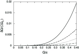
Figure 1: Particle-number violations within SCRPA for $ph$ non-symmetric cases with $\Omega=$ 10 and $\Omega_{h}=$ 1 (solid line), 2 (dashed line), 3 (dotted line), and 4 (dash-dotted line) as functions of interaction parameter $G$ (in units of the level distance $\epsilon$).

IV.2 Correlation, ground-state and excited-state energies

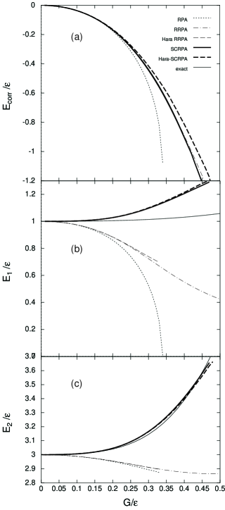
Figure 2: Correlation energy $E_{\rm corr}$ in the system with $\Omega=10$ particles (a), ground-state energy $E_{1}$ (b) and first-excited-state energy $E_{2}$ (c) of the system with $\Omega+2=$ 12 particles relative to the ground-state of $\Omega$-particle system as functions of interaction parameter $G$ obtained within RPA (dotted line), RRPA (dash-dotted line), Hara-RRPA (thin dashed line), SCRPA (thick solid line), Hara-SCRPA (thick dashed line), and exact (thin solid line) calculations.

Shown in Fig. 2 are the correlations energies of the system with $\Omega=10$ particles, as well as the energies $E_{1}$ and $E_{2}$ of the ground state and first excited state, respectively, of the system with $\Omega+2=12$ particles relative to the ground state of the $\Omega$-particle system as functions of the interaction parameter $G$ (in units of $\epsilon$). They were obtained within the RPA, RRPA, SCRPA, and are plotted in comparison with the exact results. The RRPA gives a quite good description of the correlation energy, which practically coincides with that given by the SCRPA and the exact result for $G\leq$ 0.45 MeV. However, the RRPA fails badly in describing the the ground-state $E_{1}$ and first-excited-state $E_{2}$ energies of the $\Omega+2$ system. Here, although the RRPA results do not collapse at $G_{\rm cr}\simeq$ 0.34 MeV as the RPA results do, they decrease monotonously, while the exact results as well as those given by the SCRPA increase with increasing $G$ (Cf. Refs. Dukelsky (6, 7)). The results obtained within the Hara-SCRPA are close to those given by the RRPA, but fail to converge in this model at $G>G_{\rm cr}$. The Hara-SCRRPA, which conserves the particle-number exactly in $ph$ non-symmetric cases, offers very close results to those given by the SCRPA for the $E_{1}$ and $E_{2}$ energies within the whole interval of values for $G$ under consideration. However, the correlation energy $E_{\rm corr}$ obtained within this number-conserving version of SCRPA is slightly larger than the exact result, and the discrepancy is clearly visible already starting from $G\geq$ 0.3 MeV.

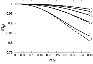
Figure 3: Ground-state correlation factor $\langle D_{p}\rangle$ for particle levels as functions of interaction parameter $G$. The solid and dashed lines denote results obtained by using Eqs. (47) and (65), respectively. The numbers next to the lines numerate the particle level, to which the lines correspond.

In general, the feature depicted in Fig. 2 is similar to that of the $ph$ case considered in Ref. CaDaSa (4), where the solution obtained by using Eq. (53) approaches the exact solution at large $G$, while the one offered by the Hara approach fails to describe it, never approaching zero. This result comes from the overestimation of ground-state correlations beyond RPA within the Hara approach, which can be clearly seen by examining the ground-state correlation factors $\langle D_{i}\rangle$ and/or the occupation number $N_{i}$. The factor $\langle D_{p}\rangle$, which is the same as $\langle D_{h}\rangle$ for the symmetric case of the picket-fence model, is shown in Fig. 3. This factor decreases from 1 with increasing $G$, approaching zero as $G\rightarrow\infty$. The deviation from 1 is stronger at the level closer to the Fermi one. The difference between the results obtained by using Eqs (53) (the SCRPA) and (65) (the Hara-SCRPA) is strongest for the lowest particle level, in which the Hara-SCRPA gives stronger ground-state correlations beyond RPA. It also increases with increasing $G$ in line with the results obtained for the $ph$ case in Ref. CaDaSa (4). This also explains the larger discrepancy between the two approaches in the description of correlation energy $E_{\rm corr}$, while the differences in the energies $E_{1}$ of the ground states, and $E_{2}$ of the first excited states are relatively smaller.

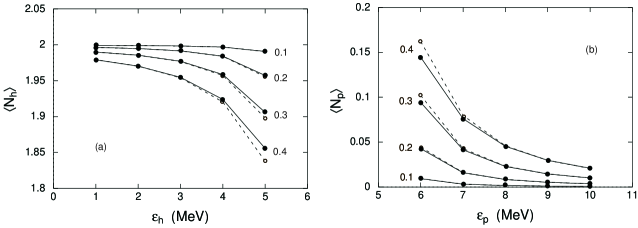
Figure 4: Occupation numbers $\langle N_{h}\rangle$ for hole levels (a) and $\langle N_{p}\rangle$ for particle levels as functions of single-particle energies $\epsilon_{i}$ at several values of $G/\epsilon$ indicated as the numbers next to the circles. The full and open circles denote results obtained by using Eqs. (47) and (65), respectively. The lines are drawn to guide the eyes.

The behavior of $\langle D_{i}\rangle$ leads to the change of the occupation number $\langle N_{p}\rangle$ and $\langle N_{h}\rangle$ as shown in Fig. 4. As small $G$, the function $N_{i}$ approaches the stair case with $\langle N_{p}\rangle\simeq$ 0 and $\langle N_{h}\rangle\simeq$ 2 for all $\epsilon_{i}$. As $G$ increases, the deviation from the stair case becomes more and more evident with the decrease of $\langle N_{h}\rangle$ from 2 and increase of $\langle N_{p}\rangle$ from 0. At $G/\epsilon=$ 0.4, e.g, $\langle N_{h}\rangle$ becomes 1.85 and $\langle N_{p}\rangle$ reaches 0.4 for levels closest to the Fermi one. The deviation caused by the Hara-SCRPA is always stronger than that given by the SCRPA. Since $\langle D_{i}\rangle\rightarrow$ 0 as $G\rightarrow\infty$ we have from Eq. (65) (the Hara-SCRPA) the sum $\sum_{\lambda}(Y_{p}^{\lambda})^{2}=\sum_{\mu}(Y_{h}^{\mu})^{2}\rightarrow 1/2$, which make $N_{p}=N_{h}\rightarrow$ 1. For the SCRPA at the value $\sum_{\lambda}(Y_{p}^{\lambda})^{2}=\sum_{\mu}(Y_{h}^{\mu})^{2}=1/2$ one obtains $\langle D_{p}\rangle=\langle D_{h}\rangle=1/2$, which lead to $\langle N_{p}\rangle=1/2$ and $\langle N_{h}\rangle=3/2$. Again, this shows that ground-state correlations beyond RPA are stronger within Hara-SCRPA than within SCRPA.

Table 1: Correlation energy $E_{\rm corr}$, ground-state energy $E_{1}$, and first-excited-state energy $E_{2}$ obtained within the “parametrized” Hara-SCRPA using Eq. (67) with $\alpha=$ 1.9 (a) in comparison with those given by the SCRPA (b) for $\Omega=$ 10. All the values are given in MeV.

	$E_{\rm corr}$		$E_{1}$		$E_{2}$
$G$	a	b	a	b	a	b
0.01	$-0.3265\times 10^{-3}$	$-0.3265\times 10^{-3}$	1.0000	1.0000	3.0000	3.0000
0.05	$-0.9018\times 10^{-2}$	$-0.8563\times 10^{-2}$	1.0005	1.0005	3.0001	3.0001
0.10	$-0.3850\times 10^{-1}$	$-0.3652\times 10^{-1}$	1.0032	1.0033	3.0063	3.0063
0.15	$-0.9263\times 10^{-1}$	$-0.8808\times 10^{-1}$	1.0111	1.0112	3.0194	3.0194
0.20	$-0.1760$	$-0.1686$	1.0278	1.0279	3.0811	3.0460
0.25	$-0.2930$	$-0.2846$	1.0566	1.0563	3.0922	3.0926
0.30	$-0.4470$	$-0.4424$	1.0985	1.0970	3.1645	3.1657
0.35	$-0.6401$	$-0.6475$	1.1514	1.1481	3.2670	3.2703
0.40	$-0.8823$	$-0.9023$	1.2118	1.2058	3.4011	3.4087
0.45	$-1.1608$	$-1.2094$	1.2755	1.2667	3.5654	3.5804

The exaggeration of the ground-state correlations beyond RPA within the renormalization procedure, which leads to the number-conserving (Hara) type expressions (65) was pointed out before by Rowe in Ref. Rowe (2), where, by using the number-operator method to insert the number operator twice at the center of $\langle N_{i}\rangle$, he found that the $ph$ ground-state correlation factor $\langle\langle D_{ph}\rangle\rangle$ became $\sum_{\nu}|Y_{ph}^{\nu}|^{2}$ instead of $2\sum_{\nu}|Y_{ph}^{\nu}|^{2}$. The result of an infinite expansion by inserting repeatedly the number operator at the center of $\langle N_{i}\rangle$ is not available for $pp$RPA at this stage. However, the observation by Rowe suggested that the real $\langle D_{p}\rangle$ and $\langle D_{h}\rangle$ might be closer to 1 than those given by Eqs. (65). Therefore, a test was also carried out here by parametrizing $\langle D_{p}\rangle$ and $\langle D_{h}\rangle$ within the Hara-SCRPA to see if it is possible to achieve results as good as those given by SCRPA for all three quantities $E_{\rm corr}$, $E_{1}$ and $E_{2}$. For this test, we used

$$\langle\widetilde{D}_{p}\rangle=1-\alpha\sum_{\lambda}(Y_{p}^{\lambda})^{2}~{},\hskip 14.22636pt\langle\widetilde{D}_{h}\rangle=1-\alpha\sum_{\mu}(Y_{h}^{\mu})^{2}~{},\hskip 14.22636pt\alpha<2~{},$$ (67)

instead of Eqs. (65) and repeated the calculations. The result of this test shows that the values $E_{\rm corr}$, $E_{1}$, and $E_{2}$ obtained within the SCRPA can be fitted simultaneously rather well within such “parametrized” Hara-SCRPA with the parameter $\alpha\simeq$ 1.9 . These results are shown in Table 1 in comparison with the SCRPA ones. Such “parametrized” Hara-SCRPA also conserves exactly the particle number in the $ph$ non-symmetric case as the Hara-SCRPA does.

V Conclusions

The present work shows that the SCRPA violates the particle number in the $ph$ non-symmetric case if the occupation numbers are calculated according to Eq. (46) for the picket-fence model, which is a limit of Eq. (51) for the general shell-model spherical basis. Within the $ph$ non-symmetric picket-fence model this particle-number violation increases with the asymmetry and interaction strength $G$, but it decreases with increasing the particle number. However, within the interval of values for $G$ under consideration ($G\leq$ 0.5 MeV), we also found that the particle-number violation reaches at most around 0.2$\%$ for the most asymmetric case with the level number $\Omega=10$, where the number of hole levels $\Omega_{h}=1$, and number of particle levels $\Omega_{p}=9$ . In all other less asymmetric cases this violation is smaller than 0.1$\%$.

In order to maintain the exact particle-number conservation within the SCRPA, a renormalization was proposed, which represents the number operator in terms of the product of renormalized pairing operators. As a result, a number-conserving SCRPA was derived, which is called Hara-SCRPA as it has the equations for the occupation numbers similar to what obtained in the pioneering works by Hara et al. but for $ph$ case Hara (1). The results of numerical calculations show that the Hara-SCRPA yields the ground state energy and energy of the first excited state of the $\Omega+2$ system very close to the corresponding values obtained within the SCRPA. However, the correlation energy, which the Hara-SCRPA offers, is slightly larger than that obtained within SCRPA.

The results of the present study also indicate that, in realistic calculations using non-symmetric single-particle spectra within RPA, in particular for light systems, one should carefully examine the violation of Pauli principle to see if it is important to include the ground-state correlations beyond RPA. As a matter of fact, the preliminary results of RRPA calculations, which were carried out recently for ^12,14Be using the Gogny interaction VMD (9), have shown that ground-state correlations beyond RPA increased the correlation energy by 20 – 24$\%$ compared to the RPA results. This shifted up the ground state energy by 13$\%$ for ¹²Be and 48$\%$ for ¹⁴Be. At the same time the particle-number violation within the RRPA due to the use of Eq. (51) did not exceed 0.2$\%$. In this case the SCRPA can be still well justified, and has the advantage over the Hara-SCRPA as the former offers a better description of the correlation energy.

In the cases where the particle-number violation cannot be neglected (e.g. $>1\%$) in calculations with realistic spectra and interactions a number-conserving approach like the Hara-SCRPA proposed in the present work might have to be used instead of the SCRPA. However, the improvement of the correlation energy in this case cannot be achieved by simply renormalizing RPA as has been done in the approaches under discussion. The test of parametrizing the Hara-SCRPA to yield all the three energies $E_{\rm corr}$, $E_{1}$, and $E_{2}$ close to the values given by the SCRPA suggests that higher-order correlations may have to be included in order to reproduce all these three quantities within a number-conserving SCRPA. This indicates coupling to configurations more complicated than the $ph$, $pp$, or $hh$ ones should also be taken into account.

References

• (1) K. Hara, Prog. Theor. Phys. 32, 88 (1964), K. Ikeda, T. Udagawa, and H. Yamamura, Prof. Theor. Phys. 33, 22 (1965).
• (2) D.J. Rowe, Phys. Rev. 175, 1283 (1968).
• (3) P. Schuck and S. Ethofer, Nucl. Phys. A 212, 269 (1973)
• (4) F. Catara, N.D. Dang, and M. Sambataro, Nucl. Phys. A 579, 1 (1994).
• (5) J. Dukelsky, P. Schuck, Nucl. Phys. A 512 466, (1990); J. Dukelsky, G. Roepke, and P. Schuck, Nucl. Phys. A 628, 17 (1998).
• (6) J. Dukelsky and P. Schuck, Phys. Let. B464, 164 (1999).
• (7) J.G. Hirsch, A. Mariano, J. Dukelsky, and P. Schuck, Ann. Phys. 296, 187 (2002) (See also arXiv:nucl-th/0109036v1 13 Sep. 2001).
• (8) J.C. Pacheco and N. Vinh Mau, Phys. Rev. C 65, 044004 (2002).
• (9) N. Dinh Dang and N. Vinh Mau, (2004) unpublished.