Direct Urca neutrino radiation from superfluid baryonic matter

Abstract

Dense matter in compact stars cools efficiently by neutrino emission via the direct Urca processes $n\to p+e+\bar{\nu}_{e}$ and $p+e\to n+\nu_{e}$. Below the pairing phase transition temperature $T_{c}$ these processes are suppressed - at asymptotically low temperatures exponentially. We compute the emissivity of the Urca process at one loop for temperatures $T\leq T_{c}$, in the case where the baryons are paired in the ${}^{1}S_{0}$ partial wave. The Urca process is suppressed linearly, rather than exponentially, within the temperature range $0.1\leq T/T_{c}\leq 1$. The charge-current Cooper pair-breaking process contributes up to $50\%$ of the total Urca emissivity in this temperature range.

1 Introduction and summary

The direct Urca process (single neutrino $\beta$-decay) was introduced in astrophysics by Gamow and Schoenberg in their studies of stellar collapse and supernova explosions [1]. In a newly born neutron star, the proton fraction drops to a few percent of the net density at the end of the deleptonization phase. At such low concentrations of charged particles the energy and momentum can not be conserved in a weak charged current decay of a single (on-shell) particle because of the large mismatch between the Fermi energies of baryons, therefore the direct Urca process is forbidden. The two-baryon processes are not constrained kinematically [2], and the so-called modified Urca process $n+n\to n+p+e+\bar{\nu}_{e}$ is the main source of neutrino emission at low proton concentrations. Boguta [3] and Lattimer et al. [4] pointed out that the high density matter can sustain large enough proton fraction ($\geq 11\%-13\%$ according to ref. [4]) for the Urca process to work. The proton fraction in dense matter is controlled by the symmetry energy of the neutron rich nuclear matter which is not well constrained. Exotic states of matter open new channels of rapid cooling with neutrino emission rates comparable to the direct Urca rate [5].

Below $T_{c}$ pair correlations open a gap ($\Delta$) in the quasiparticle spectrum of baryons. At low temperatures, when the width of the energy states accessible to quasiparticles due to the temperature smearing of the Fermi-surfaces is less than the gap in the quasiparticle spectrum, the neutrino production by the direct Urca process is quenched by a factor ${\rm exp}(-\Delta/T)$, where $\Delta$ is the larger of the neutron and proton gaps. At moderate temperatures $T\leq T_{c}$, the changes in the phase-space occupation caused by the gaps in the quasiparticle spectra are non-exponential; and the weak decay matrix elements acquire coherence pre-factors, since the degrees of freedom (the Bogolyubov quasiparticles) are a superposition of the particles and holes describing the unpaired state. The phase space changes due to the pairing were cast in suppression factors multiplying the emissivity of the processes in the normal state in refs. [7]; the role of coherence factors has not been studied so far.

Our aim below is to compute the direct Urca emissivity in the superfluid phases of dense nucleonic matter below $T_{c}$. We start by expressing the neutrino emissivity of the direct Urca process in terms of the polarization tensor of matter within the real-time Green’s functions approach to the quantum neutrino transport [8]. (The derivation in Section 2 applies to a larger class of charge current reactions involving $\beta$-decay; an example is the modified Urca process). The polarization tensor is then computed at one-loop for the isospin asymmetric nuclear matter where the $S$-wave pairing is among the same-isospin quasiparticles. Within the range of temperatures $0.1\leq T/T_{c}\leq 1$ the suppression of the Urca process will turn out to be linear rather than exponential in temperature. An additional contribution to the Urca process comes from (previously ignored) charge-current pair-breaking process. Both the charge-neutral current counterparts of the pair-breaking processes [9, 10, 11] and the direct Urca processes (suppressed by pair-correlations below $T_{c}$) were found important in numerical simulations of compact star cooling [12, 13, 14, 15, 16, 17, 18, 19]. Below, we shall treat the baryonic matter as non-relativistic Fermi-liquid; one should keep in mind, however, that the relativistic mean-field treatments differ quantitatively from their non-relativistic counterparts [20, 21].

2 Propagators and self-energies

Stellar matter is approximately in equilibrium with respect to the weak processes - the $\beta$-decay and electron capture rates are nearly equal. Thus, we need to compute the rate of, say, anti-neutrino production by neutron $\beta$-decay and multiply the final result by a factor of 2. We start with the transport equation for anti-neutrinos [8]

$$\left[\partial_{t}+\vec{\partial}_{q}\,\omega_{\bar{\nu}}({\mbox{\boldmath$q$}})\vec{\partial}_{X}\right]f_{\bar{\nu}}({\mbox{\boldmath$q$}})=\int^{0}_{-\infty}\frac{dq_{0}}{2\pi}{\rm Tr}\left[\sigma^{<}(q)S_{\bar{\nu}}^{>}(q)-\sigma^{>}(q)S_{\bar{\nu}}^{<}(q)\right],$$ (1)

where $f_{\bar{\nu}}({\mbox{\boldmath$q$}})$ is the anti-neutrino Wigner function, $S_{\bar{\nu}}^{>,<}(q)$ and $\sigma^{>,<}(q)$ are their propagators and self-energies, $\omega_{\bar{\nu}}({\mbox{\boldmath$q$}})=|{\mbox{\boldmath$q$}}_{\bar{\nu}}|$ is the on-mass-shell anti-neutrino energy and $q=(q_{0},{\mbox{\boldmath$q$}})$ is the four-momentum. The Wigner function, propagators and self-energies depend on the center-of-mass coordinate $X$, which is implicit in Eq. (1). If the leptons are on-shell and massless, their propagators are related to their Wigner functions via the quasiparticle ansatz [8]

$$S_{\lambda}^{<}(q) = \frac{i\pi\!\not\!q}{\omega_{\lambda}({\mbox{\boldmath$q$}})}\Big{\{}\delta\left(q_{0}-\omega_{\lambda}({\mbox{\boldmath$q$}})\right)f_{\lambda}(q)-\delta\left(q_{0}+\omega_{\bar{\lambda}}({\mbox{\boldmath$q$}})\right)\left[1-f_{\bar{\lambda}}(-q)\right]\Big{\}},$$ (2)

where the index $\lambda=\nu,\,\,e$ refers to neutrino ($\nu$) and electron ($e$) and $\bar{\lambda}=\bar{\nu},\,\,\bar{e}$ to anti-neutrino ($\bar{\nu}$) and positron ($\bar{e}$). Both neutrinos and electrons obey a linear dispersion relation $\omega_{\lambda}=|{\mbox{\boldmath$q$}}_{\lambda}|$, since the electron neutrino mass can be ignored on energy scales $\sim 10^{2}$ keV, while the electrons are ultrarelativistic at relevant densities. In addition to the propagator $S_{\lambda}^{<}(q)$ we will need the “time-reversed” propagator $S_{\lambda}^{>}(q)$ which is obtained from (2) by an interchange of the particle and hole distributions $f_{\lambda}(q)\leftrightarrow 1-f_{\lambda}(q).$

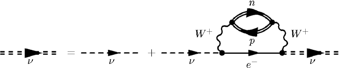
Figure 1: The diagrammatic Dyson equation for neutrinos which defines the self-energies $\sigma^{>,<}(q)$. The free and full neutrino propagators are shown by the dashed and double dashed lines, the electrons and paired baryons - by the solid and double-solid lines; the wavy lines correspond to the gauge $W^{+}$-boson propagator. According to Eq. (2), the neutrino Green’s function simultaneously propagates a neutrino and anti-neutrino hole; the time-reversed Green’s function propagates a anti-neutrino and a neutrino hole.

The standard model neutrino-baryon charged-current interaction is

$$V=\frac{\tilde{G}}{\sqrt{2}}J^{(H)}\,J^{(L)},\quad J^{(H)}_{\mu}=\overline{\phi}\gamma_{\mu}(c_{V}-c_{A}\gamma_{5})\phi,\quad J_{(L)}^{\mu}=\overline{\psi}\gamma^{\mu}(1-\gamma_{5})\psi,$$ (3)

where $\tilde{G}\equiv G_{F}\cos\theta$ with $G_{F}$ being the weak coupling constant and $\theta$ the Cabibbo angle ($\cos\theta=0.973$), $\psi$ and $\phi$ are the neutrino and baryon field operators, $c_{V}$ and $c_{A}$ are the weak charged-current vector and axial vector coupling constants. The neutrino self-energies $\sigma^{>,<}(q)$ can be evaluated perturbatively with respect to the weak interaction. To lowest order in $\tilde{G}$ the second-order Born diagram gives (see Fig. 1)

$$-i\sigma^{>,<}(q_{1}) = \sum_{q,q_{2}}\delta^{4}(q_{1}-q_{2}+q)~{}i\Gamma_{(L)}^{\mu}~{}iS_{e}^{<}(q_{2})~{}i\Gamma_{(L)}^{\dagger\,\zeta}~{}i\Pi^{<,>}_{\mu\zeta}(q),$$ (4)

where $\sum_{q}\equiv\int d^{4}q/(2\pi)^{4}$ is the phase-space integration symbol, $\Pi^{>,<}_{\mu\zeta}(q)$ is the baryon polarization tensor and $\Gamma_{\mu(L)}=\gamma_{\mu}(1-\gamma_{5})$ is the weak interaction vertex, which is independent of $q$ at the energy and momentum transfers much smaller than the gauge boson mass. Substituting the self-energies and the propagators in the collision integral we find for the loss part [the second term on the r.-h. side of Eq. (1)]

$$I_{\bar{\nu}}^{>}({\mbox{\boldmath$q$}}_{1})=i\int^{0}_{-\infty}\!\!\frac{dq_{10}}{2\pi}\sum_{q,q_{2}}\delta^{4}(q_{1}-q_{2}+q)~{}{\rm Tr}\left[~{}\Gamma^{\mu}_{(L)}\frac{\pi\!\not\!q_{2}}{\omega_{e}({\mbox{\boldmath$q$}}_{2})}\Gamma^{\dagger\,\zeta}_{(L)}\frac{\pi\!\not\!q_{1}}{\omega_{\bar{\nu}}({\mbox{\boldmath$q$}}_{1})}\right]$$

$$\delta\left(q_{02}-\omega_{e}({\mbox{\boldmath$q$}}_{2})\right)\left[1-f_{e}(q_{2})\right]\delta\left(q_{10}+\omega_{\bar{\nu}}({\mbox{\boldmath$q$}}_{1})\right)\left[1-f_{\bar{\nu}}(q_{1})\right]\Pi_{\mu\zeta}^{<}(q),$$ (5)

where we retained from the collision integral the only relevant term which has an electron and anti-neutrino in the final state. The gain term naturally does not contribute to the emission rate.

3 Direct Urca emissivities

The anti-neutrino emissivity (the energy radiated per unit time) is obtained from Eq. (1)

$$\epsilon_{\bar{\nu}} = \frac{d}{dt}\int\!\frac{d^{3}q}{(2\pi)^{3}}f_{\bar{\nu}}({\mbox{\boldmath$q$}})\omega_{\bar{\nu}}({\mbox{\boldmath$q$}}).$$ (6)

Carrying out the energy integrations in Eq. (2) and using the equilibrium identity $\Pi_{\mu\zeta}^{<}(q)=2ig_{B}(q_{0}){\Im{\rm m}}\,\Pi_{\mu\zeta}^{R}(q)$, where $g_{B}(q_{0})$ is the Bose distribution function and $\Pi^{R}_{\mu\zeta}(q)$ is the retarded polarization function, we obtain

$$\epsilon_{\bar{\nu}} = -2\left(\frac{\tilde{G}}{\sqrt{2}}\right)^{2}\int\!\frac{d^{3}q_{1}}{(2\pi)^{3}2\omega_{e}({\mbox{\boldmath$q$}}_{1})}\int\!\frac{d^{3}q_{2}}{(2\pi)^{3}2\omega_{\bar{\nu}}({\mbox{\boldmath$q$}}_{2})}\int\!d^{4}q\,\delta({\mbox{\boldmath$q$}}_{1}+{\mbox{\boldmath$q$}}_{2}-{\mbox{\boldmath$q$}})$$ (7)

$$\delta(\omega_{e}+\omega_{\bar{\nu}}-q_{0})\,\omega_{\bar{\nu}}({\mbox{\boldmath$q$}}_{2})g_{B}(q_{0})\left[1-f_{e}(\omega_{e})\right]\Lambda^{\mu\zeta}(q_{1},q_{2})\Im{\rm m}\,\Pi^{R}_{\mu\zeta}(q),$$

where $\Lambda^{\mu\zeta}(q_{1},q_{2})={\rm Tr}\left[\gamma^{\mu}(1-\gamma^{5})\!\not\!q_{1}\gamma^{\zeta}(1-\gamma^{5})\!\not\!q_{2}\right]$. The symbol $\Im{\rm m}$ refers to the imaginary part the polarization tensor’s resolvent. Since the baryonic component of stellar matter is in thermal equilibrium to a good approximation, it is convenient to use the Matsubara Green’s functions (ref. [23], pg. 120)

$$G_{\sigma\sigma^{\prime}}({\mbox{\boldmath$p$}},\tau) = -\delta_{\sigma\sigma^{\prime}}\langle T_{\tau}a_{p\sigma}(\tau)a^{\dagger}_{p\sigma^{\prime}}(0)\rangle,$$

$$F_{\sigma\sigma^{\prime}}({\mbox{\boldmath$p$}},\tau) = \langle T_{\tau}a_{-p\downarrow}(\tau)a_{p\uparrow}(0)\rangle,\quad\quad F^{\dagger}_{\sigma\sigma^{\prime}}({\mbox{\boldmath$p$}},\tau)=\langle T_{\tau}a_{p\uparrow}^{\dagger}(\tau)a^{\dagger}_{-p\downarrow}(0)\rangle,$$ (8)

where $\tau$ is the imaginary time, $a^{\dagger}_{p\sigma}(\tau)$ and $a_{p\sigma}(\tau)$ are the creation and destruction operators, $\sigma=\uparrow,\downarrow$ stands for spin and the propagators are diagonal in the isospin space. The quasiparticle spectra of Cooper pairs coupled in a relative $S$-wave state are (the wave-vectors $p$ and $k$ refer to protons and neutrons) $\epsilon_{p}=\sqrt{\xi_{p}^{2}+\Delta_{p}^{2}}$, $\epsilon_{k}=\sqrt{\xi_{k}^{2}+\Delta_{n}^{2}}$ with (omitting the isospin index) $\xi={p^{2}}/{2m}+{\Re{\rm e~{}}}\Sigma(p)-\mu$, where $\mu$, $m$ and $\Sigma(p)$ are the chemical potentials, masses and self-energies of protons and neutrons. Expanding the self-energy around the Fermi-momentum $p_{F}$ leads to $\xi={p^{2}}/{2m^{*}}-\mu^{*},$ where $\mu^{*}=-{\Re{\rm e~{}}}\Sigma(p_{F})+\mu,$ and $m/m^{*}=(1+\partial\Re{\rm e~{}}\Sigma(p)/\partial p|_{p=p_{F}})$.

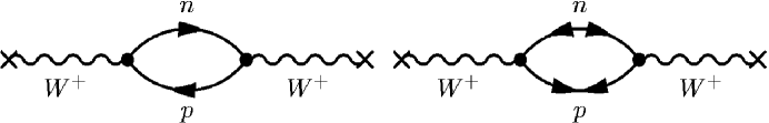
Figure 2: The one loop baryon polarization tensor. The baryon and (amputated) $W^{+}$-boson propagators are shown by the solid and wave lines. The double arrow lines refer to the anomalous propagators (ref. [23], pg. 300).

The density and spin-density response functions are defined in terms of imaginary-time ordered products ($T_{\tau}$ is the ordering symbol)

$$\Pi({\mbox{\boldmath$q$}},iq_{0}) = \sum_{\sigma,\sigma^{\prime},p,p^{\prime}}\int_{0}^{\beta}d\tau e^{i\omega\tau}\alpha\cdot\alpha^{\prime}\langle T_{\tau}a^{\dagger}_{p+q,\sigma}(\tau)a_{p,\sigma}(\tau)a^{\dagger}_{p^{\prime}-q,\sigma^{\prime}}(0)a_{p^{\prime},\sigma^{\prime}}(0)\rangle,$$ (9)

where $\alpha=1$ for the vector and $\sigma$ for the axial vector response ($\sigma$ is the vector of Pauli matrices). The one-loop density-density and spin-spin correlation functions are given by

$$\Pi_{V/A}({\mbox{\boldmath$q$}},iq_{0})=\frac{1}{\beta}\sum_{\sigma p}\left[G({\mbox{\boldmath$p$}},ip)G({\mbox{\boldmath$k$}},ik_{0})\mp F({\mbox{\boldmath$p$}},ip)F^{\dagger}({\mbox{\boldmath$k$}},ik_{0})\right],$$ (10)

where $p=(ip_{0},{\mbox{\boldmath$p$}})$, $k=(ip_{0}+iq_{0},{\mbox{\boldmath$p$}}+{\mbox{\boldmath$q$}})$, the zeroth components of these four-vectors are the complex fermionic Matsubara frequencies, and $\beta$ is the inverse temperature. The different signs in Eq. (10) reflect the fact that under time reversal the $\alpha$ vertex is even for scalar and odd for spinor perturbations. Note that the one-loop approximation above ignores the vertex corrections, which can be treated within the Fermi-liquid theory [22]. The summation over the Matsubara frequencies in (10) followed by analytical continuation gives

$$\Pi_{V/A}^{R}({\mbox{\boldmath$q$}},\omega) = \sum_{\sigma,\vec{p}}\Biggl{\{}\left(\frac{u_{p}^{2}u_{k}^{2}\mp u_{p}u_{k}v_{p}v_{k}}{\omega+\epsilon_{p}-\epsilon_{k}+i\delta}-\frac{v_{p}^{2}v_{k}^{2}\mp u_{p}u_{k}v_{p}v_{k}}{\omega-\epsilon_{p}+\epsilon_{k}+i\delta}\right)\left[f(\epsilon_{p})-f(\epsilon_{k})\right]$$ (11)

$$+\left(\frac{u_{p}^{2}v_{k}^{2}\pm u_{p}u_{k}v_{p}v_{k}}{\omega-\epsilon_{p}-\epsilon_{k}+i\delta}-\frac{u_{p}^{2}v_{k}^{2}\pm u_{p}u_{k}v_{p}v_{k}}{\omega+\epsilon_{p}+\epsilon_{k}+i\delta}\right)\left[f(-\epsilon_{p})-f(\epsilon_{k})\right]\Biggr{\}},$$

where $u_{p}^{2}=(1/2)\left(1+|\xi_{p}|/\epsilon_{p}\right)$ and $u_{p}^{2}+v_{p}^{2}=1$. The first term in Eq. (11) describes the quasiparticle scattering, which is the generalization to superfluids of the ordinary scattering in the unpaired state; the second one describes pair-breaking, which is specific to superfluids. Taking the imaginary part and changing to dimensionless variables $y=\beta\omega$, $x=\beta\xi_{p}$ and $w_{i}=\beta\Delta_{i}$ ($i=p,n$) we obtain

$${\rm Im}\Pi_{V/A}^{R}(q,y) = -\frac{m_{n}^{*}m_{p}^{*}}{2\pi q\beta}\left[{I}^{SC}_{V/A}(y)+{I}^{PB}_{V/A}(y)\right],$$ (12)

where the (dimensionless) integrals for the vector (V) and axial vector (A) couplings are

$${I}^{SC/PB}_{V}(y) = \int_{-\infty}^{\infty}dx~{}{C}^{SC/PB}_{V}(x,y,w_{p})|\Xi^{SC/PB}(x,y,w_{n})|$$ (13)

$$\times \left[f(\pm\sqrt{x^{2}+w_{p}^{2}})-f(\sqrt{x^{2}+w_{p}^{2}}+y)\right]\theta(1-|x_{0}^{\pm}|).$$

where $\Xi^{SC/PB}(x,y,w_{n})=(\omega\pm\epsilon_{p})\left\{|(\omega\pm\epsilon_{p})^{2}-\Delta_{n}^{2}|\right\}^{-1/2}$, and

$$x_{0}^{\pm}={\rm sgn}(\omega\pm\epsilon_{p})\frac{m_{n}^{*}}{pq}\left\{\sqrt{|(\omega\pm\epsilon_{p})^{2}-\Delta_{n}^{2}|}-l^{2}\right\}$$ (14)

with $l^{2}\equiv(p^{2}+q^{2})/(2m_{n}^{*})-\mu_{n}^{*}$. The axial-vector integrals ${I}^{SC/PB}_{A}$ are obtained by replacing in (13) the coherence factors ${C}^{SC/PB}_{V}$ by ${C}^{SC/PB}_{A}$, where $C^{SC}_{V/A}=(u_{p}u_{k}\mp v_{p}v_{k})^{2},$ and $C^{PB}_{V/A}=u_{k}^{2}v_{p}^{2}\pm u_{p}u_{k}v_{p}v_{k}.$ On substituting Eq. (12) in Eq. (7) we obtain

$$\epsilon_{\bar{\nu}} = -8\tilde{G}^{2}\frac{m_{n}^{*}m_{p}^{*}}{2\pi\beta}\int\!\frac{d^{4}q}{q}~{}g_{B}(\omega)\left[({I}^{SC}_{V}+{I}^{PB}_{V})+3g_{A}^{2}({I}^{SC}_{A}+{I}^{PB}_{A})\right]\int\!\frac{d^{3}q_{1}}{(2\pi)^{3}2\omega_{e}}$$ (15)

$$\times \int\!\frac{d^{3}q_{2}}{(2\pi)^{3}2\omega_{\bar{\nu}}}\left[1-f_{e}(\omega_{e})\right]\delta^{3}({\mbox{\boldmath$q$}}_{1}+{\mbox{\boldmath$q$}}_{2}-{\mbox{\boldmath$q$}})\delta(\omega_{e}+\omega_{\bar{\nu}}-\omega)\,\omega_{\bar{\nu}}^{2}\omega_{e},$$

where the (unquenched) axial coupling constant $g_{A}=1.26$. Since the neutrino momentum is much smaller than the electron Fermi-momentum, ${\mbox{\boldmath$q$}}\simeq{\mbox{\boldmath$q$}}_{1}$ and $|q_{1}|\simeq p_{Fe}$. With this approximation our final result is

$$\epsilon_{\bar{\nu}} = \frac{3\tilde{G}^{2}m_{n}^{*}m_{p}^{*}p_{Fe}}{2\pi^{5}\beta^{6}}J=\epsilon_{0}J,$$ (16)

$$J = -\frac{1}{6}\int_{-\infty}^{\infty}\!dy~{}g_{B}(y)\left[({I}^{SC}_{V}+{I}^{PB}_{V})+3g_{A}^{2}({I}^{SC}_{A}+{I}^{PB}_{A})\right]\int_{0}^{\infty}dzz^{3}f_{e}(z-y).$$

The second integral can be expressed through the polylogarithmic function ${\rm Li}_{4}[-{\rm exp}(y)]$, though this is not particularly illuminating. Above $T_{c}$ Eq. (16) yields the finite-temperature emissivity of the direct Urca process

$$\epsilon_{\bar{\nu}}=(1+3g_{A}^{2})\epsilon_{0}\int\!dy~{}g_{B}(y)~{}{\rm ln}\frac{1+e^{-x_{\rm min}}}{1+e^{-(x_{\rm min}+y)}}\int dzz^{3}f_{e}(z-y),$$ (17)

where $x_{\rm min}=\beta(p_{\rm min}^{2}/2m^{*}-\mu_{p}^{*})$ and $p_{\rm min}=(m^{*}/q)(\omega-\mu_{p}^{*}+\mu_{n}^{*}-q^{2}/2m^{*})$ [here we assume $m_{n}^{*}\simeq m_{p}^{*}=m^{*}$]. At zero temperature the logarithm in Eq. (17) reduces to $y\theta(-x_{\rm min})$, the integrals are analytical and one easily recovers the zero-temperature result of ref. [4].

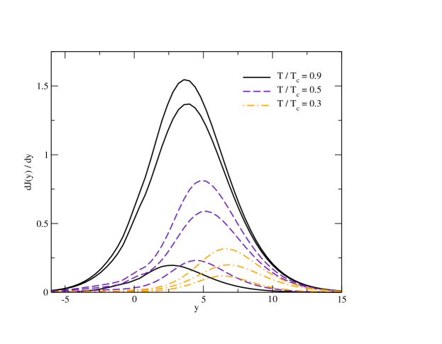
Figure 3: The energy distribution of the neutrino radiation $dJ(y)/dy$ for $T/T_{c}=0.9$ (solid lines), 0.5 (dashed lines), 0.3 (dashed dotted lines). For each fixed $T/T_{c}$ the lines correspond to (bottom to top) the pair-breaking, scattering and total contributions.

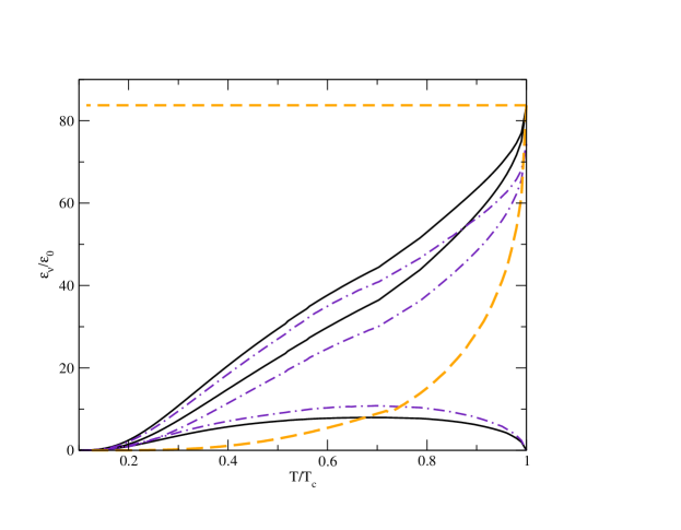
Figure 4: The neutrino emissivity in units of $\epsilon_{0}$ versus temperature (solid lines $\Delta_{n}(0)=\Delta_{p}(0)=0.5$ MeV, dashed-dotted lines $\Delta_{n}(0)=0.5,$ $\Delta_{p}(0)=2$ MeV). The scattering, pair-breaking contributions and their sum are shown by dashed and dashed-dotted and solid lines. The upper short-dashed line is the extrapolation of the rate for unpaired matter to low temperatures, the lower one corresponds to the exponential suppression as discussed in the text.

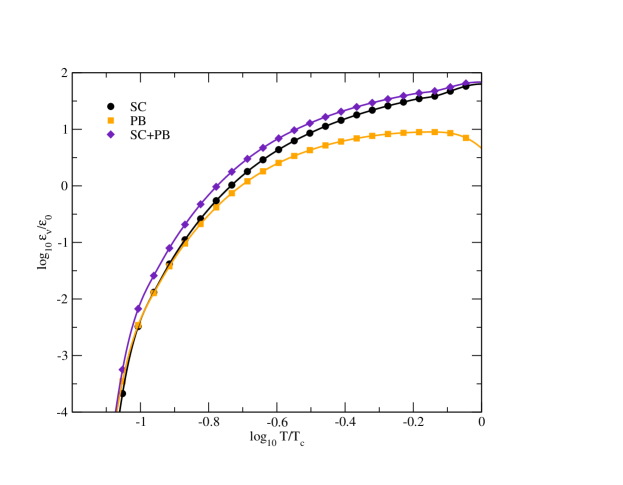
Figure 5: The log-log plot of the dependence of the neutrino emissivity in units of $\epsilon_{0}$ on temperature. The scattering, pair-breaking contributions and their sum are marked by circles, squares, and diamonds respectively.

4 A model calculation

To set-up an illustrative model, we assume $\Delta_{n}(T=0)=\Delta_{p}(T=0)=0.5$ MeV, $m_{n}^{*}/m_{n}=m_{p}^{*}/m_{p}=0.7$, $\Re{\rm e~{}}\Sigma(p_{Fn})=-10$ MeV and $\Re{\rm e~{}}\Sigma(p_{Fp})=-160$ MeV at the density 0.24 fm^-3, which is above the Urca threshold in charge neutral nucleonic matter under $\beta$-equilibrium for the assumed values of the baryon self-energies. The neutron self-energy shift is taken more repulsive than the one found in non-relativistic calculations with two-body interactions to mimic the effect of repulsive three-body forces. The remaining parameters of the model are $p_{Fn}=1.8$ fm^-1, $p_{Fp}=p_{Fe}=1.07$ fm^-1, $\mu_{n}^{*}=96.3$ MeV, $\mu_{p}^{*}=34.2$ MeV and $\mu_{e}=212.1$ MeV.

Fig. 3 shows the energy distribution of the neutrino radiation $dJ(y)/dy$ for various temperatures. The energy distribution is thermal with the maximum at $\omega\sim 3T$ in agreement with the fact that each anti-neutrino carries on average energy equal to $3T$ in units of Boltzmann constant. For smaller $T/T_{c}$ the maximum shifts to larger energies corresponding to higher “effective temperature” and the peak of the distribution is reduced because of pairing; the thermal shape of the distribution remains unchanged. While in the limit $T/T_{c}\leq 1$ the scattering contribution dominates, at lower temperatures the pair-breaking process becomes increasingly important; e.g. at $T/T_{c}\sim 0.3$ it contributes about the half of the scattering contribution.

Fig. 4 focuses on the temperature dependence of the direct neutrino emissivity in the range $0.1\leq T/T_{c}\leq 1$. The important feature here is the nearly linear dependence of the emissivity on the temperature in the range $0.1\leq T/T_{c}\leq 1$; the commonly assumed exponential decay - a factor exp($-\Delta/T$) with $\Delta={\rm max}(\Delta_{n},\Delta_{p})$ - underestimates the emissivity. (Similar conclusion concerning the suppression of the direct Urca process by pair correlations was reached in ref. [7] which treated the scattering contribution to the emissivity). The contribution of the pair-breaking processes becomes substantial in the low-temperature range $0.1\leq T/T_{c}\leq 0.4$ (about the half of the scattering contribution at $T/T_{c}\sim 0.3$). Increasing the value of the proton gap to 2 MeV while keeping the neutron gap at its value 0.5 MeV suppresses the emissivity of the scattering process, since at a given temperature the phase space accessible to the excited states is reduced. The pair-breaking processes are almost unaffected since they are related to the scattering of particles in and out-of the condensate. The temperature dependence of the net emissivity can be crudely approximated as $\epsilon_{\bar{\nu}}=90\,\epsilon_{0}\,(T/T_{c}-0.1)$; this reduces to the standard Urca result for $T=T_{c}$ and sufficiently well (for the purpose of cooling simulations) reproduces the numerical result in Fig. 3 for $T/T_{c}\in[0.1;1]$. Alternatively the rate of the Urca process in the unpaired matter can be suppressed by a factor $(10/9)(T/T_{c}-0.1)$. Fig 5 illustrates the low-temperature asymptotics of the emissivities for $\Delta_{n}=\Delta_{p}=0.5$ MeV. For $T/T_{c}\leq 0.1$ the contribution of the pair-breaking process to the total emissivity is equal or larger than that of the scattering one. Asymptotically, the logarithmic derivative of the emissivity, $d{\rm log}\,\epsilon_{\nu}/d{\rm log}\,T$, tends to a constant (negative) value which depends only on the magnitude(s) of the zero temperature gap(s), as should be the case for exponentially suppressed emissivities.

References

- [1] G. Gamow, M. Schoenberg, Phys. Rev. 59 (1941) 539.
- [2] The modified Urca process was originally studied in H. Y. Chiu, E. E. Salpeter, Phys. Rev. Lett. 12 (1964) 413; J. N. Bahcall and R. A. Wolf, Phys. Rev. Lett. 14, (1965) 343; Phys. Rev. 140, B1452. The recent work on these processes is described in D. N. Voskresensky, Lecture Notes in Physics vol. 578, Springer, Berlin, 2001, p. 467 [astro-ph/0009093] and D. G. Yakovlev, C. J. Pethick, Ann. Rev. Astron. Astrophys. 42 (2004) 169.
- [3] J. Boguta, Phys. Lett. B 106 (1981) 255.
- [4] J. M. Lattimer, C. J. Pethick, M. Prakash, P. Haensel, Phys. Rev. Lett. 66 (1991) 2701.
- [5] C. J. Pethick, Rev. Mod. Phys. 64 (1992) 1133 and referencies therein.
- [6] A. Sedrakian and U. Lombardo, Phys. Rev. Lett. 84 (2000) 602.
- [7] K. P. Levenfish, D. G. Yakovlev, Astron. Lett. 20 (1994) 43 [Pis’ma Astron. Zh. 20 (1994) 54]; D. G. Yakovlev, K. P. Levenfish, Yu. A. Shibanov, Sov. Phys. Usp. 169 (1999) 825, Sec. 4.
- [8] A. Sedrakian and A. E. L. Dieperink, Phys. Rev. D 62 (2000) 083002.
- [9] E. G. Flowers, M. Ruderman, P. G. Sutherland, Astrophys. J. 205 (1976) 541.
- [10] D. N. Voskeresensky, A. V. Senatorov, Sov. J. Nucl. Phys., 45 (1987) 411 [ Yad. Fiz. 45 (1987) 657].
- [11] D. G. Yakovlev, A. D. Kaminker, K. P. Levenfish, Astron. Astrophys. 343 (1999) 650.
- [12] C. Schaab, D. Voskresensky, A. Sedrakian, F. Weber, M. Weigel, Astron. Astrophys. 321 (1997) 591.
- [13] C. Schaab, A. Sedrakian, F. Weber, M. Weigel, Astron. Astrophys. 346 (1999) 465.
- [14] D. Page, In: Neutron Stars and Pulsars, ed. N. Shibazaki, N. Kawai, S. Shibata, T. Kifune, p.183 (Universal Academy press, Tokyo 1998) [astro-ph/9802171].
- [15] D. Page, J. M. Lattimer, M. Prakash, A. Steiner, Ap. J. suppl., in press, [astro-ph/0403657].
- [16] D. Page, preprint (2004) [astro-ph/0405196].
- [17] A. D. Kaminker, P. Haensel, D. G. Yakovlev, Astron. Astrophys. 383 (2001) L17.
- [18] S. Tsuruta, M. A. Teter, T. Takatsuka, T. Tatsumi, R. Tamagaki, Ap. J. 571 (2002) L143.
- [19] D. Blaschke, H. Grigorian, D. Voskresensky, Astron. Astrophys. 424 (2004) 979.
- [20] L. B. Leinson, A. Pérez, Phys. Lett. B 518 (2001) 15; Phys. Lett. B 522 (2001) 358, Erratum.
- [21] L. B. Leinson, Nucl. Phys. A 707 (2002) 543.
- [22] D. N. Voskeresensky, A. V. Senatorov, JETP 63 (1986) 885 [Zh. Eksp. Teor. Fiz. 90 (1986) 1505].
- [23] A. A. Abrikosov, L. P. Gorkov, I. E. Dzyaloshinkski, Methods of quantum field theory in statistical physics, (Dover, New York, 1975).