Low-energy constants and relativity in
peripheral nucleon-nucleon scattering

Abstract

In our recent works we derived a chiral $O(q^{4})$ two-pion exchange nucleon-nucleon potential (TPEP) formulated in a relativistic baryon (RB) framework, expressed in terms of the so called low energy constants (LECs) and functions representing covariant loop integrations. We showed that the expansion of these functions in powers of the inverse of the nucleon mass reproduces most of the terms of the TPEP derived from the heavy baryon (HB) formalism, but such an expansion is ill defined and does not converge at large distances. In the present work we perform a study of the phase shifts in nucleon-nucleon ($NN$) scattering for peripheric waves ($L\geq 3$), which are sensitive to the tail of the potential. We assess quantitatively the differences between the RB and HB results, as well as variations due to different values of the LECs. By demanding consistency between the LECs used in $\pi N$ and $NN$ scattering we show how $NN$ peripheral phase shifts could constrain these values. We demonstrate that this idea, first proposed by the Nijmegen group, favors a smaller value for the LEC $c_{3}$ than the existing ones, when considering the TPEP up to order $q^{4}$ in the chiral expansion.

I Introduction

One of the most intriguing mysteries in the history of modern physics is trying to describe and understand nuclear forces in terms of a basic, elementary theory of strong interactions. Despite more than fifty years of intense research in this area only in the last decade such a connection could be established, between what is believed to be the theory of strong interactions, QCD, and the rich phenomenology of low-energy nuclear physics. Chiral symmetry plays an essencial role in this game. Weinberg wein79 first pointed out that it can be used to obtain not only the same predictions of current algebra c-algeb , but also corrections to them. Later these ideas were systematically elaborated by Gasser and Leutwyler chpt , evolving to what is known as chiral perturbation theory (ChPT). It relies on the fact that the QCD lagrangian exhibits chiral $SU(N_{f})\times SU(N_{f})$ symmetry, $N_{f}$ being the number of light quarks ($u$, $d$, and, eventually, $s$ quarks), in the limit where their masses, $m_{q}$, go to zero. This underlying theory is then described effectively including the relevant degrees of freedom (pions and nucleons for the case we are interested in, $N_{f}=2$) in the most generic way constrained only by the allowed symmetries, and caracterized by an expansion parameter $q$ representing either the momenta involved or the symmetry breaking terms $m_{q}\propto\mu^{2}$, $\mu$ being the Goldstone boson (pion) mass. The effective theory is then evaluated by means of feynman diagrams, strictly obeying a given power counting scheme. These ideas were successfuly applied to many processes in the mesonic sector, forming a compelling evidence that ChPT indeed represents QCD in the low-energy regime ecker ; bkmeis95 ; scherer02 .

The power counting is an essential ingredient in ChPT, allowing us to evaluate corrections in a consistent and controlled way. In the mesonic sector it follows naturally, once loop contributions are regularized using dimensional regularization. On the other hand, with baryons an additional energy scale (the baryon mass) is introduced, which does not vanish in the chiral limit and makes the theory much more complicated, with chiral loops (using dimensional regularization) spoiling the power counting gss . For many years it was believed that a relativistic treatment of baryons in ChPT was not consistent with power counting. The first and widely used formalism which restores the latter consists in applying a sort of non-relativistic expansion at the level of the lagrangian, around the limit of infinitely heavy baryon (HBChPT), proposed by Jenkins and Manohar in the early 90s jenkman . Almost ten years later, Becher and Leutwyler bl99 ; bl01 showed that it is possible to formulate baryonic ChPT preserving explicit Lorentz invariance and power counting (RBChPT). Based on previous works of Ellis and Tang EllisT , the so called infrared regularization allows one to not only remove the power counting violating terms from loop integrals, but also recover the results from HBChPT when subjected to an expansion in powers of the inverse of the baryon mass. From the latter, Becher and Leutwyler showed that the heavy baryon approach fails to preserve the correct analytic structure of the theory in a specific low energy domain. In $\pi N$ scattering, this region corresponds to the Mandelstam variable $t$ close to $4\mu^{2}$. This motivated further studies inside the covariant framework fuchs ; lutz ; goity .

In recent works nos1 ; nos2 we brought the issue of HBChPT and RBChPT to the two-pion exchange nucleon-nucleon potential (TPEP), showing that its long distance properties are governed by the same low energy region where the HBChPT has convergence problems. In nos1 we also performed an expansion of our results in powers of $1/m$ ($m$ being the nucleon mass) and compared with the HB expressions from Entem and Machleidt EM , where we found a small number of differences. These works triggered the importance to assess quantitatively the differences between the HB- and RB-ChPT $NN$ potentials in asymptotic phase shifts, and if they are comparable to the uncertainties in the parameters of the potential, the so called low energy constants (LECs). The discrepancies found between our expanded nos1 and the HB EM expressions also needs to be understood as they should, in principle, coincide. It is the main goal of this work to address both issues.

The determination of the LECs is of much current interest, as they describe the dynamics of QCD at low energies. At the order we are working on, it requires the knowledge of the dimension two ($c_{i}$) and three ($d_{i}$) LECs, present at the order $q^{2}$ (${\cal L}^{(2)}_{N}$) and order $q^{3}$ (${\cal L}^{(3)}_{N}$) pion-nucleon chiral Lagrangians, respectively. Obviously, it seems more natural trying to obtain their values from $\pi N$ processes. In Ref. bkm97 it was performed through a fit to threshold and subthreshold parameters, and a physical interpretation for their values was given, similar to what has been done in the pure mesonic sector ecker89 . For instance, assuming that the LEC $c_{1}$ is entirely saturated by a scalar meson exchange, a perfect agreement for their mass and coupling constant with the ones used by the Bonn one boson exchange model bonn emerges. The other dimension two LECs $c_{2}$, $c_{3}$, and $c_{4}$ where also estimated to be dominated by the delta resonance, with relevant contributions from rho ($c_{4}$) and sigma ($c_{3}$) mesons, and marginal contributions from the Roper resonance $N^{*}$(1440). However, description of $\pi N$ phase shifts, albeit consistent, was not satisfactory, the same happening with the values from Mojžiš moj98 ; datpak . It was improved in subsequent papers fms98 ; butik , but the central values for the LECs still vary considerably evg02 . Moreover, the most reasonable results were obtained using the experimental analyses from the Karlsruhe group kochpiet ; ka84 , which show disagreements with most recent $\pi N$ database. As an alternative to $\pi N$ processes, recently the Nijmegen group proposed the extraction of the dimension two LECs $c_{1}$, $c_{3}$, and $c_{4}$ using $NN$ partial wave analyses nij99 ; nij03 , where they obtained values with (statistical) uncertainties much smaller than obtained from $\pi N$ processes. Their values were disputed by Entem and Machleidt EM ; EMach-com , and in this work we also try to investigate this question.

An important point here is that we do not try to address details of the non-perturbative aspect of the $NN$ interaction; instead, we deal only with the two-nucleon irreducible diagrams up to order $q^{4}$, which should be identified with the irreducible kernel in a Bethe-Salpeter equation, or the potential in a Lippmann-Schwinger equation. As suggested by Weinberg wein90 , the usual power counting of ChPT should be applied to it. The reducible diagrams are afflicted with infrared divergences (or, in the language of old-fashioned time-ordered perturbation theory, small energy denominators) and, depending on the power counting adopted, a resumation of certain classes of diagrams have to be performed to all orders. The non-perturbative problem is dealt in the more generic framework of effective field theory (EFT, for reviews see, for instance, Refs. bbhps00 ; kubod99 ; eftrev ; lepage ) and, despite of the progress it has achieved in the last years bira ; egm ; egm04-1 ; egm04-2 ; bgr99 ; cgk04 ; va04 there are still controversies about power counting schemes wein90 ; ksw ; fms ; bk02 ; gege ; YH04 . This work follows the same spirit as the ones from Kaiser et.al. KBW ; Kaiser2 ; Kaiser3 , Entem and Machleidt EM , and Ballot, Rocha, and Robilotta BRR , in the sense that we look only at peripheral waves ($l\geq 3$) where the Born approximation is expected to be valid BR ; egm04-1 . With this procedure we try to investigate how far we are from the dream of establish, as in the case of the one-pion exchange (OPE) in the mid-60s, a mathematical structure for the two-pion exchange (TPE) which can be called “unique”, dictaded by chiral symmetry (by unique here we do not consider ambiguities arising from off-shell effects cf86 or choices of field variables egm , as discussed in Ref. friar99 ).

We organize this paper as follows. In Sec. II we present the motivation of our previous works with some detail, showing the contrast between RB and HB calculations for the TPEP. There we also address the differences we found when comparing our expanding results with the HB expressions, and their origin are better (but still not completely) understood. An interesting outcome of this work is a quantitative measure of how different ranges of the potential contributes to the phase shifts, and this was made possible by the use of the phase function (or variable phase) method, described in Sec. III. This study, as well as the dependence of the phase shifts with some of the existing values for the LECs, is shown in Sec. IV, where we found some restrictions in order to achieve consistency with the experimental data. We close this work with our conclusions and remarks in Sec. V.

II relativistic versus heavy baryon TPEP

In our recent works nos1 ; nos2 we argued that the problem of convergence that appears in the HB formulation manifests itself in the TPEP at large distances. This was ilustrated by comparing our basic loop functions with their $1/m$ expansion, the latter not being able to reproduce the correct asymptotic behavior. In the end of this section we show that the same occurs to the TPEP decomposed in peripheral partial waves ($J\geq 3$). Before that, we present a discussion about the differences we found between our expanded results and the ones obtained in the HB framework KBW ; Kaiser2 ; Kaiser3 ; EM . It is worth to emphasize that they must in principle coincide, therefore, such discrepancies should not exist. To investigate them we revised some of our calculations, and updated results are presented in Secs. II.2 and II.3. In order to fix the notation and help understanding the origin of these discrepancies we outline the main steps on the derivation of our TPEP. For further details, we direct the reader to our previous works nos1 ; nos2 . For numerical evaluations, in this section we use the same values for the LECs used by Entem and Machleidt EM (last column of table 3).

II.1 formalism

Figure 1: The irreducible two-pion exchange amplitude.

The TPE contribution to the $NN$ interaction can be parametrized in terms of $\pi N$ scattering sub-amplitudes, as ilustrated by the first graph on the right hand side of Fig. 1. One can describes the $\pi N$ scattering in terms of two invariant amplitudes $D^{\pm}(\nu,t)$ and $B^{\pm}(\nu,t)$,

$$T_{\pi N}^{ab} = \delta_{ab}\,T_{\pi N}^{+}+i\epsilon_{bac}\,\tau_{c}\,T_{\pi N}^{-}\,,$$

$$T_{\pi N}^{\pm} = \bar{u}({\mbox{\boldmath$p^{\prime}$}})\,\Big{[}D^{\pm}-\frac{i}{2m}\,\sigma_{\mu\nu}(p^{\prime}-p)^{\mu}\,\frac{(k+k^{\prime})^{\nu}}{2}\,B^{\pm}\Big{]}\,u({\mbox{\boldmath$p^{\prime}$}})\,,$$ (1)

where $m$ is the nucleon mass, with initial and final momenta $p$ and $p^{\prime}$, respectively, while $\nu=[(p+k)^{2}-(p-k^{\prime})^{2}]/4m$ and $t=(k^{\prime}-k)^{2}$ are the usual Mandelstam variables. This allows the TPE amplitude to be written as

$${\cal T}_{TPE} = -\frac{i}{2!}\int[\cdots]\left[3\,T_{\pi N}^{(1)+}\,T_{\pi N}^{(2)+}+2\,{\mbox{\boldmath$\tau$}}^{(1)}\cdot{\mbox{\boldmath$\tau$}}^{(2)}\,T_{\pi N}^{(1)-}\,T_{\pi N}^{(2)-}\right]$$ (3)

$$= \left[\bar{u}u\right]^{(1)}\left[\bar{u}u\right]^{(2)}{\cal I}_{DD}^{\pm}$$

$$-\left[\bar{u}u\right]^{(1)}\left[\bar{u}\,i\,\sigma_{\mu\lambda}\,\frac{(p^{\prime}-p)^{\mu}}{2m}\,u\right]^{(2)}{\cal I}_{DB}^{\lambda\pm}-\left[\bar{u}\,i\,\sigma_{\mu\lambda}\,\frac{(p^{\prime}-p)^{\mu}}{2m}\,u\right]^{(1)}\left[\bar{u}u\right]^{(2)}{\cal I}_{DB}^{\lambda\pm}$$

$$+\left[\bar{u}\,i\,\sigma_{\mu\lambda}\,\frac{(p^{\prime}-p)^{\mu}}{2m}\,u\right]^{(1)}\left[\bar{u}\,i\,\sigma_{\nu\rho}\,\frac{(p^{\prime}-p)^{\nu}}{2m}\,u\right]^{(2)}{\cal I}_{BB}^{\lambda\rho\pm}\,,$$

where the symbol $\int[\cdots]$ represents the four-dimensional integration with two pion propagators,

$$\int[\cdots]=\int\frac{d^{4}Q}{(2\pi)^{4}}\,\frac{1}{(k^{2}-\mu^{2})}\,\frac{1}{(k^{\prime 2}-\mu^{2})}\,,$$ (4)

$\mu$ is the pion mass, $Q=(k+k^{\prime})/2$, and the profile functions ${\cal I}$’s are loop integrals written in terms of the amplitudes $D^{\pm}$ and $B^{\pm}$,

$$\begin{array}[]{rclcrcl}{\cal I}_{DD}^{\pm}&=&-\frac{i}{2}\,\int[\cdots]\,D^{(1)\pm}\,D^{(2)\pm}\,,&{\mbox{\ \ \ \ }}&{\cal I}_{DB}^{\lambda\pm}&=&-\frac{i}{2}\,\int[\cdots]\,Q^{\lambda}\;D^{(1)\pm}\,B^{(2)\pm}\,,\\[5.69054pt] {\cal I}_{BD}^{\lambda\pm}&=&-\frac{i}{2}\,\int[\cdots]\,Q^{\lambda}\;B^{(1)\pm}\,D^{(2)\pm}\,,&&{\cal I}_{BB}^{\lambda\rho\pm}&=&-\frac{i}{2}\,\int[\cdots]\,Q^{\lambda}Q^{\rho}\;B^{(1)\pm}\,B^{(2)\pm}\,.\end{array}$$ (5)

Using the variables

$$W=p_{1}+p_{2}=p^{\prime}_{1}+p^{\prime}_{2}\,,\qquad z=\frac{1}{2}\,\big{[}(p_{1}+p^{\prime}_{1})-(p_{2}+p^{\prime}_{2})\big{]}\,,\qquad q=k^{\prime}-k=p^{\prime}_{1}-p_{1}=p_{2}-p^{\prime}_{2}\,,$$ (6)

we decompose the Lorentz structure of these profile functions as

$${\cal I}_{DB}^{\lambda\pm} = \frac{W^{\lambda}}{2m}\,{\cal I}_{DB}^{(w)\pm}+\frac{z^{\lambda}}{2m}\,{\cal I}_{DB}^{(z)\pm}\,,$$ (7)

$${\cal I}_{BD}^{\lambda\pm} = \frac{W^{\lambda}}{2m}\,{\cal I}_{DB}^{(w)\pm}-\frac{z^{\lambda}}{2m}\,{\cal I}_{DB}^{(z)\pm}\,,$$ (8)

$${\cal I}_{BB}^{\lambda\rho\pm} = g^{\lambda\rho}\,{\cal I}_{BB}^{(g)\pm}+\frac{W^{\lambda}W^{\rho}}{4m^{2}}\,{\cal I}_{BB}^{(w)\pm}+\frac{z^{\lambda}z^{\rho}}{4m^{2}}\,{\cal I}_{BB}^{(z)\pm}\,.$$ (9)

The evaluation of Eq.(5) to leading order gives rise to bubble, triangle, crossed box, and plannar box diagrams, the latter one containing an iteration of the one pion exchange (OPE). In order to obtain the irreducible TPE amplitude, this contribution has to be subtracted. Schematically it is represented by Fig. 2, where the symbol “+” on the second graph means that the two-nucleon propagator contains only its positive-energy projection. This projection is not uniquely defined RAP99 ; friar99 and several prescriptions, like the Blankenbecler-Sugar BbS , Equal-Time EqT , or the Gross Gross equations, could be used. Therefore, when comparing our expanded results with the HB ones, we should keep in mind that part of the differences might come from the particular prescription adopted.

Figure 2: The plannar box diagram (left) and the positive-energy projection of the iterated OPE (right), which has to be subtracted to obtain the irreducible TPE amplitude.

The iterated OPE can be recasted in the same structure as Eq.(3), allowing us to define the functions $\hat{\cal I}$’s as the ones in Eq.(5) subtracted by the iterated OPE amplitude. The components of the potential, up to $O(q^{4})$, can therefore be written in terms of these functions as

$$V_{C}^{\pm} = \tau^{\pm}\,\frac{m}{E}\Biggl{\{}\hat{\cal I}_{DD}^{\pm}+\frac{q^{2}}{4m^{2}}\left[2\,\hat{\cal I}^{(w)\pm}_{DB}-\hat{\cal I}_{DD}^{\pm}\right]$$ (10)

$$\!+\frac{q^{2}}{4m^{2}}\biggl{[}\frac{q^{2}}{4m^{2}}\left(\hat{\cal I}^{(w)\pm}_{BB}-2\,\hat{\cal I}^{(w)\pm}_{DB}+\hat{\cal I}^{(g)\pm}_{BB}\right)-\frac{z^{2}}{4m^{2}}\left(\frac{1}{4}\,\hat{\cal I}_{DD}^{\pm}+\hat{\cal I}^{(w)\pm}_{DB}+\hat{\cal I}^{(z)\pm}_{DB}\right)\biggr{]}\Biggr{\}}\,,$$

$$V_{LS}^{\pm} = \tau^{\pm}\,\frac{m}{E}\Biggl{\{}-\frac{1}{2}\,\hat{\cal I}_{DD}^{\pm}+\hat{\cal I}^{(z)\pm}_{DB}+\hat{\cal I}^{(w)\pm}_{DB}+\frac{q^{2}}{4m^{2}}\left[-\frac{1}{2}\,\hat{\cal I}^{(z)\pm}_{DB}+\frac{3}{2}\,\hat{\cal I}^{(g)\pm}_{BB}-\frac{3}{2}\,\hat{\cal I}^{(w)\pm}_{DB}+\frac{1}{8}\,\hat{\cal I}_{DD}^{\pm}+\hat{\cal I}^{(w)\pm}_{BB}\right]$$ (11)

$$-\frac{z^{2}}{4m^{2}}\left[\frac{1}{2}\,\hat{\cal I}^{(z)\pm}_{DB}+\frac{1}{2}\,\hat{\cal I}^{(w)\pm}_{DB}+\frac{1}{8}\,\hat{\cal I}_{DD}^{\pm}\right]\Biggr{\}}\,,$$

$$V_{T}^{\pm} = \frac{1}{2}\,V_{SS}^{\pm}=\tau^{\pm}\,\frac{m}{E}\Biggl{[}-\frac{1}{12}\,\hat{\cal I}^{(g)\pm}_{BB}\Biggr{]}\,,$$ (12)

$$V_{Q}^{\pm} = \!\tau^{\pm}\,\frac{m}{E}\Biggl{\{}-\frac{1}{64}\,\hat{\cal I}_{DD}^{\pm}+\frac{1}{16}\,\hat{\cal I}^{(z)\pm}_{DB}-\frac{1}{8}\,\hat{\cal I}^{(g)\pm}_{BB}+\frac{1}{16}\,\hat{\cal I}^{(w)\pm}_{DB}+\frac{1}{16}\,\hat{\cal I}^{(z)\pm}_{BB}-\frac{1}{16}\,\hat{\cal I}^{(w)\pm}_{BB}\Biggr{\}}\,.$$ (13)

The dynamics of our relativistic TPEP is classified in terms of three families of diagrams, according to their topology. The first line of diagrams in Fig. 3 corresponds to the irreducible one loop graphs with vertices from the $O(q^{1})$ $\pi N$ chiral Lagrangian, ${\cal L}^{(1)}_{\pi N}$, with coupling constants at their physical values (family I). The second line (family II) contains two loop diagrams with an intermediate $\pi\pi$ scattering, while the third line (family III) comprises one loop graphs with vertices from ${\cal L}^{(2)}_{\pi N}$ and ${\cal L}^{(3)}_{\pi N}$, as well as other two loop graphs, parametrized in terms of $\pi N$ subthreshold coefficients hoeler .

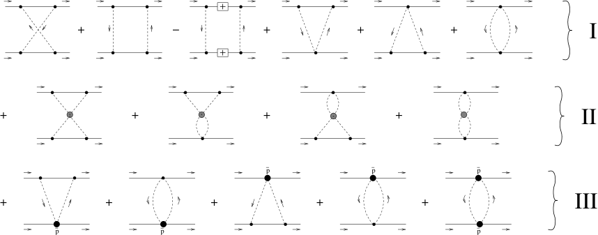
Figure 3: Dynamics of the relativistic TPEP. The small black dots represent vertices from ${\cal L}^{(1)}_{\pi N}$, the big shaded dots, the $\pi\pi$ scattering amplitude, and the big black dots, the $\pi N$ subthreshold coefficients. The latter contains other two loop contributions, as well as vertices from ${\cal L}^{(2)}_{\pi N}$ and ${\cal L}^{(3)}_{\pi N}$.

II.2 revision of our two loop diagrams

The expressions for our previous profile functions are given in appendices D–F of Ref. nos1 . While investigating the origin of the differences between our expanded and the HB results, we realize a small mistake in our two loop contributions (family II). We checked that the revised calculation is independent on the parametrization of the pion field and leads to

$${\cal I}^{+}_{DD} = -\frac{1}{(4\pi)^{4}}\,\frac{\mu^{4}g_{A}^{4}}{16f_{\pi}^{6}}\,(1-2t/\mu^{2})\,\Big{[}(1-t/2\mu^{2})\,\Pi_{t}-2\pi\Big{]}^{2}\,,$$ (14)

$${\cal I}^{-}_{DD} = -\frac{1}{(4\pi)^{4}}\,\frac{\mu^{4}}{4f_{\pi}^{6}}\;\frac{W^{2}}{4m^{2}}\,\Bigg{\{}\frac{1}{3}\,(g_{A}^{2}-1)\bigg{[}(1-t/4\mu^{2})\,\Pi_{\ell}+2-\frac{t}{4\mu^{2}}\bigg{]}-g_{A}^{2}\bigg{[}(1-t/2\mu^{2})\,\Pi_{\ell}+1-\frac{t}{3\mu^{2}}\bigg{]}\Bigg{\}}^{2}\,,$$ (15)

$${\cal I}^{(g)-}_{BB} = -\frac{1}{(4\pi)^{4}}\,\frac{m^{2}\mu^{2}}{4f_{\pi}^{6}}\,\Big{[}g_{A}^{2}\,(1-t/4\mu^{2})\,\Pi_{t}-\pi\Big{]}^{2}\,,$$ (16)

$${\cal I}^{(g)+}_{BB} = {\cal I}^{(z)\pm}_{DB}={\cal I}^{(w)\pm}_{BB}={\cal I}^{(w)\pm}_{BB}={\cal I}^{(w)\pm}_{DB}=0\,,$$ (17)

where $g_{A}$ and $f_{\pi}$ are respectively the nucleon axial coupling and the pion decay constant, and $\Pi_{\ell}$, $\Pi_{t}$, $\Pi_{\times}$, $\Pi_{b}$, $\tilde{\Pi}_{b}$, and $\Pi_{a}$ are our basic loop integrals defined in Ref. nos1 . These modifications alter the expressions of just two components of our non-expanded, relativistic potential: in $V_{C}^{-}$, the non-local (nonstatic) term

$$\left[\frac{\mu}{m}\right]^{2}\frac{m^{2}}{256\pi^{2}f_{\pi}^{2}}\,\frac{z^{2}}{\mu^{2}}\,g_{A}^{4}\left[\left(1-\frac{t}{4\mu^{2}}\right)\Pi_{t}-\pi\right]^{2}$$ (18)

does not exist, while in $V_{LS}^{-}$ there are no contributions from family II at all.

II.3 $1/m$ expansion and analysis of discrepancies

The second revision we made concerns the HB expansion of our loop functions. We found that the plannar and crossed box integrals ($\Pi_{b}$ and $\Pi_{\times}$, respectively) which, in Ref. nos1 , were given by

$$\Pi_{\times} \rightarrow -\Pi^{\prime}_{\ell}-\frac{\mu}{2m}\,\frac{\pi}{(1-t/4\mu^{2})}-\frac{\mu^{2}}{12m^{2}}\,\Big{[}3\,(1-t/2\mu^{2})^{2}\,(2\Pi^{\prime}_{\ell}-\Pi^{\prime\prime}_{\ell})+2\,(z^{2}/\mu^{2})\,\Pi^{\prime}_{\ell}\Big{]}+O(q^{3})\,,$$ (19)

$$\Pi_{b} \rightarrow -\Pi^{\prime}_{\ell}-\frac{\mu}{4m}\,\frac{\pi}{(1-t/4\mu^{2})}-\frac{\mu^{2}}{12m^{2}}\,\Big{[}(1-t/2\mu^{2})^{2}\,(2\Pi^{\prime}_{\ell}-\Pi^{\prime\prime}_{\ell})+2\,(z^{2}/\mu^{2})\,\Pi^{\prime}_{\ell}\Big{]}+O(q^{3})\;,$$ (20)

have to be corrected by

$$\Pi_{\times} \rightarrow -\Pi^{\prime}_{\ell}-\frac{\mu}{2m}\,\frac{\pi}{(1-t/4\mu^{2})}-\frac{\mu^{2}}{12m^{2}}\,\Big{[}3\,(2\Pi^{\prime}_{\ell}-\Pi^{\prime\prime}_{\ell})+2\,(z^{2}/\mu^{2})\,\Pi^{\prime}_{\ell}\Big{]}+O(q^{3})\,,$$ (21)

$$\Pi_{b} \rightarrow -\Pi^{\prime}_{\ell}-\frac{\mu}{4m}\,\frac{\pi}{(1-t/4\mu^{2})}-\frac{\mu^{2}}{12m^{2}}\,\Big{[}(2\Pi^{\prime}_{\ell}-\Pi^{\prime\prime}_{\ell})+2\,(z^{2}/\mu^{2}+t/\mu^{2})\,\Pi^{\prime}_{\ell}\Big{]}+O(q^{3})\;.$$ (22)

Therefore, the comparison of our expanded results with the HB expressions (Sec. X of Ref. nos1 ) must be updated by the following:

$$V_{C}=V_{C}^{+}=\frac{3g_{A}^{2}}{16\pi f_{\pi}^{4}}\left\{-\frac{g_{A}^{2}\;\mu^{5}}{16m(4\mu^{2}\!+\!{\mbox{\boldmath$q$}}^{2})}+\left[2\mu^{2}(2c_{1}\!-\!c_{3})-{\mbox{\boldmath$q$}}^{2}c_{3}\right](2\mu^{2}\!+\!{\mbox{\boldmath$q$}}^{2})\;A(q)\right.$$

$$\left.+\frac{g_{A}^{2}(2\mu^{2}\!+\!{\mbox{\boldmath$q$}}^{2})\;A(q)}{16m}\left[-3{\mbox{\boldmath$q$}}^{2}\;{\color[rgb]{1,0,0}\,+(4\mu^{2}\!+\!{\mbox{\boldmath$q$}}^{2})^{\dagger}}\;\right]\right\}$$

$$+\frac{g_{A}^{2}\;L(q)}{32\pi^{2}f_{\pi}^{4}m}\left\{\frac{24\mu^{6}}{4\mu^{2}\!+\!{\mbox{\boldmath$q$}}^{2}}\;(2c_{1}\!+\!c_{3})+6\mu^{4}(c_{2}\!-\!2c_{3})+4\mu^{2}{\mbox{\boldmath$q$}}^{2}(6c_{1}\!+\!c_{2}\!-\!3c_{3})+{\mbox{\boldmath$q$}}^{4}(c_{2}\!-\!6c_{3})\right\}$$

$$-\frac{3L(q)}{16\pi^{2}f_{\pi}^{4}}\left\{\left[-4\mu^{2}c_{1}\!+\!c_{3}(2\mu^{2}\!+\!{\mbox{\boldmath$q$}}^{2})+c_{2}(4\mu^{2}\!+\!{\mbox{\boldmath$q$}}^{2})/6\right]^{2}+\frac{1}{45}\,(c_{2})^{2}(4\mu^{2}\!+\!{\mbox{\boldmath$q$}}^{2})^{2}\right\}$$

$$+\frac{g_{A}^{4}}{32\pi^{2}f_{\pi}^{4}m^{2}}\left\{L(q)\left[\frac{2\mu^{8}}{(4\mu^{2}\!+\!{\mbox{\boldmath$q$}}^{2})^{2}}+\frac{8\mu^{6}}{(4\mu^{2}\!+\!{\mbox{\boldmath$q$}}^{2})}-2\mu^{4}-{\mbox{\boldmath$q$}}^{4}\right]+\frac{\mu^{6}/2}{(4\mu^{2}\!+\!{\mbox{\boldmath$q$}}^{2})}\right\}$$

$$-\frac{3g_{A}^{4}[A(q)]^{2}}{1024\pi^{2}f_{\pi}^{6}}\;(\mu^{2}\!+\!2{\mbox{\boldmath$q$}}^{2})\;(2\mu^{2}\!+\!{\mbox{\boldmath$q$}}^{2})^{2}$$

$$-\frac{3g_{A}^{4}(2\mu^{2}\!+\!{\mbox{\boldmath$q$}}^{2})\;A(q)}{1024\pi^{2}f_{\pi}^{6}}\left\{4\mu\;g_{A}^{2}\;(2\mu^{2}\!+\!{\mbox{\boldmath$q$}}^{2})+2\mu\;(\mu^{2}\!+\!2{\mbox{\boldmath$q$}}^{2})]\right\}\;,$$ (23)

$$V_{T}=-\frac{3\;V_{T}^{+}}{m^{2}}=\frac{3g_{A}^{4}\;L(q)}{64\pi^{2}f_{\pi}^{4}}-\frac{g_{A}^{4}\;A(q)}{512\pi f_{\pi}^{4}m}\left[9(2\mu^{2}+{\mbox{\boldmath$q$}}^{2})\;{\color[rgb]{1,0,0}\,+3(4\mu^{2}+{\mbox{\boldmath$q$}}^{2})^{\dagger}}\;\right]$$

$$-\frac{g_{A}^{4}\;L(q)}{32\pi^{2}f_{\pi}^{4}m^{2}}\left[{\mbox{\boldmath$z$}}^{2}/4+5{\mbox{\boldmath$q$}}^{2}/8+\frac{\mu^{4}}{4\mu^{2}\!+\!{\mbox{\boldmath$q$}}^{2}}\right]$$

$$+\frac{g_{A}^{2}\;(4\mu^{2}+{\mbox{\boldmath$q$}}^{2})\;L(q)}{32\pi^{2}f_{\pi}^{4}}\left[(\tilde{d}_{14}-\tilde{d}_{15})\;{\color[rgb]{0,0,1}\,-\left(g_{A}^{4}/32\;\pi^{2}f_{\pi}^{2}\right)^{\!*}}\;\right]\;,$$ (24)

$$V_{LS}=-\frac{V_{LS}^{+}}{m^{2}}=-\frac{3g_{A}^{4}\;A(q)}{32\pi f_{\pi}^{4}m}\;\left[(2\mu^{2}+{\mbox{\boldmath$q$}}^{2})\;{\color[rgb]{1,0,0}\,+(\mu^{2}+3{\mbox{\boldmath$q$}}^{2}/8)^{\dagger}}\;\right]$$

$$-\frac{g_{A}^{4}\;L(q)}{4\pi^{2}f_{\pi}^{4}m^{2}}\left[\frac{\mu^{4}}{4\mu^{2}\!+\!{\mbox{\boldmath$q$}}^{2}}+\frac{11}{32}\,{\mbox{\boldmath$q$}}^{2}\right]-\frac{g_{A}^{2}\;c_{2}\;L(q)}{8\pi^{2}f_{\pi}^{4}m}\;(4\mu^{2}+{\mbox{\boldmath$q$}}^{2})\;,$$ (25)

$$V_{\sigma L}=\frac{4\;V_{Q}^{+}}{m^{4}}=-\frac{g_{A}^{4}\;L(q)}{32\pi^{2}f_{\pi}^{4}m^{2}}\;,$$ (26)

$$W_{C}=V_{C}^{-}=\frac{L(q)}{384\pi^{2}f_{\pi}^{4}}\Bigg{[}4\mu^{2}\left(5g_{A}^{4}-4g_{A}^{2}-1\right)+{\mbox{\boldmath$q$}}^{2}\left(23g_{A}^{4}-10g_{A}^{2}-1\right)+\frac{48g_{A}^{4}\mu^{4}}{4\mu^{2}\!+\!{\mbox{\boldmath$q$}}^{2}}\Bigg{]}$$

$$-\frac{g_{A}^{2}}{128\pi f_{\pi}^{4}m}\Bigg{\{}\frac{3g_{A}^{2}\mu^{5}}{4\mu^{2}\!+\!{\mbox{\boldmath$q$}}^{2}}+A(q)\,(2\mu^{2}\!+\!{\mbox{\boldmath$q$}}^{2})\bigg{[}g_{A}^{2}\;(4\mu^{2}\!+\!3{\mbox{\boldmath$q$}}^{2})-2(2\mu^{2}\!+\!{\mbox{\boldmath$q$}}^{2})\;{\color[rgb]{1,0,0}\,+g_{A}^{2}(4\mu^{2}\!+\!{\mbox{\boldmath$q$}}^{2})^{\dagger}}\;\bigg{]}\Bigg{\}}$$

$$+\frac{{\mbox{\boldmath$q$}}^{2}\;c_{4}\;L(q)}{192\pi^{2}f_{\pi}^{4}m}\Big{[}g_{A}^{2}(8\mu^{2}+5{\mbox{\boldmath$q$}}^{2})+(4\mu^{2}+{\mbox{\boldmath$q$}}^{2})\Big{]}+\frac{16g_{A}^{4}\mu^{6}}{768\pi^{2}f_{\pi}^{4}m^{2}}\;\frac{1}{4\mu^{2}\!+\!{\mbox{\boldmath$q$}}^{2}}$$

$$-\frac{L(q)}{768\pi^{2}f_{\pi}^{4}m^{2}}\Bigg{\{}(4\mu^{2}\!+\!{\mbox{\boldmath$q$}}^{2}){\mbox{\boldmath$z$}}^{2}+g_{A}^{2}\Bigg{[}\frac{48\mu^{6}}{4\mu^{2}\!+\!{\mbox{\boldmath$q$}}^{2}}-24\mu^{4}-12\,(2\mu^{2}\!+\!{\mbox{\boldmath$q$}}^{2})\,{\mbox{\boldmath$q$}}^{2}+(16\mu^{2}\!+\!10{\mbox{\boldmath$q$}}^{2}){\mbox{\boldmath$z$}}^{2}\Bigg{]}$$

$$+g_{A}^{4}\Bigg{[}{\mbox{\boldmath$z$}}^{2}\Bigg{(}\frac{16\mu^{4}}{4\mu^{2}\!+{\mbox{\boldmath$q$}}^{2}}-7{\mbox{\boldmath$q$}}^{2}-20\mu^{2}\Bigg{)}-\frac{64\mu^{8}}{(4\mu^{2}\!+{\mbox{\boldmath$q$}}^{2})^{2}}-\frac{48\mu^{6}}{4\mu^{2}\!+{\mbox{\boldmath$q$}}^{2}}+\frac{16\mu^{4}{\mbox{\boldmath$q$}}^{2}}{4\mu^{2}\!+\!{\mbox{\boldmath$q$}}^{2}}+20{\mbox{\boldmath$q$}}^{4}+24\mu^{2}{\mbox{\boldmath$q$}}^{2}+24\mu^{4}\Bigg{]}\Bigg{\}}$$

$$-\frac{L(q)}{18432\pi^{4}f_{\pi}^{6}}\Bigg{\{}\Bigg{[}192\pi^{2}f_{\pi}^{2}\tilde{d}_{3}\;{\color[rgb]{0,0,1}\,-\frac{(15\!+\!7g_{A}^{4})}{5}^{\!*}}\;\Bigg{]}(4\mu^{2}\!+\!{\mbox{\boldmath$q$}}^{2})\Big{[}2g_{A}^{2}(2\mu^{2}\!+\!{\mbox{\boldmath$q$}}^{2})-3/5(g_{A}^{2}-1)(4\mu^{2}\!+\!{\mbox{\boldmath$q$}}^{2})\Big{]}$$

$$+\Big{[}6g_{A}^{2}(2\mu^{2}\!+\!{\mbox{\boldmath$q$}}^{2})-(g_{A}^{2}-1)\;(4\mu^{2}\!+\!{\mbox{\boldmath$q$}}^{2})\Big{]}$$

$$\times\Bigg{[}384\pi^{2}f_{\pi}^{2}\left((2\mu^{2}\!+\!{\mbox{\boldmath$q$}}^{2})\;(\tilde{d}_{1}+\tilde{d}_{2})+4\mu^{2}\;\tilde{d}_{5}\right)+L(q)\left(4\mu^{2}(1+2g_{A}^{2})+{\mbox{\boldmath$q$}}^{2}(1+5g_{A}^{2})\right)$$

$$-\left(\frac{{\mbox{\boldmath$q$}}^{2}}{3}\,(5+13g_{A}^{2})+8\mu^{2}(1+2g_{A}^{2})\right)\;{\color[rgb]{0,0,1}\,+\left(2g_{A}^{4}(2\mu^{2}+{\mbox{\boldmath$q$}}^{2})+\frac{2}{3}\,{\mbox{\boldmath$q$}}^{2}(1+2g_{A}^{2})\right)^{\!*}}\;\Bigg{]}\Bigg{\}}\;,$$ (27)

$$W_{T}=-\frac{3}{m^{2}}\;V_{T}^{-}=\frac{g_{A}^{2}A(q)}{32\pi f_{\pi}^{4}}\Bigg{\{}\left(c_{4}+\frac{1}{4m}\right)(4\mu^{2}\!+\!{\mbox{\boldmath$q$}}^{2})-\frac{g_{A}^{2}}{8m}\;\Big{[}10\mu^{2}+3{\mbox{\boldmath$q$}}^{2}\;{\color[rgb]{1,0,0}\,-(4\mu^{2}\!+\!{\mbox{\boldmath$q$}}^{2})^{\dagger}}\;\Big{]}\Bigg{\}}$$

$$-\frac{c_{4}^{2}\;L(q)}{96\pi^{2}f_{\pi}^{4}}(4\mu^{2}\!+\!{\mbox{\boldmath$q$}}^{2})+\frac{c_{4}\;L(q)}{192\pi^{2}f_{\pi}^{4}m}\left[g_{A}^{2}(16\mu^{2}+7{\mbox{\boldmath$q$}}^{2})-(4\mu^{2}\!+\!{\mbox{\boldmath$q$}}^{2})\right]$$

$$-\frac{L(q)}{1536\pi^{2}f_{\pi}^{4}m^{2}}\left[g_{A}^{4}\left(28\mu^{2}+17{\mbox{\boldmath$q$}}^{2}+\frac{16\;\mu^{4}}{4\mu^{2}\!+\!{\mbox{\boldmath$q$}}^{2}}\right)-g_{A}^{2}(32\mu^{2}+14{\mbox{\boldmath$q$}}^{2})+(4\mu^{2}\!+\!{\mbox{\boldmath$q$}}^{2})\right]$$

$$-\frac{[A(q)]^{2}g_{A}^{4}\;(4\mu^{2}\!+\!{\mbox{\boldmath$q$}}^{2})^{2}}{2048\pi^{2}f_{\pi}^{6}}-\frac{A(q)g_{A}^{4}\;(4\mu^{2}\!+\!{\mbox{\boldmath$q$}}^{2})}{1024\pi^{2}f_{\pi}^{6}}\;\mu(1+2g_{A}^{2})\;,$$ (28)

$$W_{LS}=-\frac{1}{m^{2}}\;V_{LS}^{-}=\frac{A(q)}{32\pi f_{\pi}^{4}m}\Big{[}g_{A}^{2}\,(g_{A}^{2}-1)\;(4\mu^{2}+{\mbox{\boldmath$q$}}^{2})\;{\color[rgb]{1,0,0}\,+g_{A}^{4}\;(2\mu^{2}+3{\mbox{\boldmath$q$}}^{2}/4)^{\dagger}}\;\Big{]}$$

$$+\frac{c_{4}\;L(q)}{48\pi^{2}mf_{\pi}^{4}}\Big{[}g_{A}^{2}(8\mu^{2}+5{\mbox{\boldmath$q$}}^{2})+(4\mu^{2}\!+\!{\mbox{\boldmath$q$}}^{2})\Big{]}$$

$$+\frac{L(q)}{256\pi^{2}m^{2}f_{\pi}^{4}}\Bigg{[}(4\mu^{2}\!+\!{\mbox{\boldmath$q$}}^{2})-16g_{A}^{2}\;(\mu^{2}+3{\mbox{\boldmath$q$}}^{2}/8)+\frac{4g_{A}^{4}}{3}\Bigg{(}9\mu^{2}+11{\mbox{\boldmath$q$}}^{2}/4-\frac{4\mu^{4}}{4\mu^{2}+{\mbox{\boldmath$q$}}^{2}}\Bigg{)}\Bigg{]}\;,$$ (29)

$$W_{\sigma L}\simeq 0\;,$$ (30)

where $L(q)$ is the usual logaritmic function,

$$L(q)=-\frac{1}{2}\,\Pi_{\ell}=\frac{\sqrt{4\mu^{2}+q^{2}}}{q}\,\ln\frac{\sqrt{4\mu^{2}+q^{2}}+q}{2\mu}$$ (31)

and, from now on, $q=|{\mbox{\boldmath$q$}}|$.

We can notice that the number of different terms dropped from 14 in Ref. nos1 down to 9. Now we have a better understanding about their origins: those marked with ${\color[rgb]{1,0,0}[\cdots]^{\dagger}}$ (six terms) are related to our choice of the Blankenbecler-Sugar BbS prescription to deal with the iterated OPEP, which is the same adopted in Refs. nos1 ; nos2 ; RR ; BRR ; BR . Different prescriptions lead to different expressions only for these terms, as mentioned previously. In the HB calculations of Refs. KBW ; Kaiser3 , the plannar box diagram is expanded in powers of $1/m$ and then the iterated OPEP (given by Eq.(20) of Ref. KBW ) is identified and subtracted. A more detailed study of these aspects will be given elsewhere future .

The remaining three different terms, marked with ${\color[rgb]{0,0,1}[\cdots]^{\!*}}$, are originated from two loop contributions of Kaiser2 , part of them parametrized in our calculations through the subthreshold coefficients (family III). The one in $V_{T}$ (and, consequently, $V_{S}$), Eq.(24), can roughly be identified with the unintegrated term $V_{T}^{(b)}$ of Ref. EM , which was not considered while performing the above comparison. In order to show that this can be the case, notice first that their structures are similar. The HB expressions from Entem and Machleidt read

$$V_{T}^{(a)}(q) = \frac{g_{A}^{2}}{32\pi^{2}f_{\pi}^{4}}\,{\mbox{\boldmath$q$}}^{4}\,\int_{2\mu}^{\infty}\frac{4d\alpha}{\alpha^{4}(\alpha^{2}+{\mbox{\boldmath$q$}}^{2})}\,3\kappa^{3}\int_{0}^{1}dx(1-x^{2})\,(\bar{d}_{14}-\bar{d}_{15})$$ (32)

$$= \frac{g_{A}^{2}L(q)}{32\pi^{2}f_{\pi}^{4}}\,(4\mu^{2}+{\mbox{\boldmath$q$}}^{2})\,(\bar{d}_{14}-\bar{d}_{15})\,,$$

$$V_{T}^{(b)}(q) = -\frac{g_{A}^{2}}{32\pi^{2}f_{\pi}^{4}}\left[\frac{g_{A}^{4}}{32\pi^{2}f_{\pi}^{2}}\right]{\mbox{\boldmath$q$}}^{4}\,$$ (33)

$$\times \int_{2\mu}^{\infty}\frac{4d\alpha}{\alpha^{4}(\alpha^{2}+{\mbox{\boldmath$q$}}^{2})}\,2\kappa^{3}\int_{0}^{1}dx(1-x^{2})\,\Bigg{[}\,\frac{1}{6}-\frac{\mu^{2}}{\kappa^{2}x^{2}}+\Bigg{(}1+\frac{\mu^{2}}{\kappa^{2}x^{2}}\Bigg{)}^{3/2}\ln\,\frac{\kappa x+\sqrt{\mu^{2}+\kappa^{2}x^{2}}}{\mu}\,\Bigg{]}\,,$$

where $\kappa\equiv\sqrt{\alpha^{2}/4-\mu^{2}}$. Our equivalent terms are

$$V_{T}^{(a)}(q) = \frac{g_{A}^{2}L(q)}{32\pi^{2}f_{\pi}^{4}}\,(4\mu^{2}+{\mbox{\boldmath$q$}}^{2})\,(\bar{d}_{14}-\bar{d}_{15})\,,$$ (34)

$$V_{T}^{(b)}(q) = -\frac{g_{A}^{2}L(q)}{32\pi^{2}f_{\pi}^{4}}\,(4\mu^{2}+{\mbox{\boldmath$q$}}^{2})\left[\frac{g_{A}^{4}}{32\pi^{2}f_{\pi}^{2}}\right]\,.$$ (35)

In the first and second columns of table 1 we display, respectively, the values of Eqs.(35) and (33) in configuration space, as a function of the internucleon distance $r$. We can see that the difference between them decreases with $r$, being around 20% at 1fm, 10% at 2fm, and remaining in a few % for $r\geq 3$fm. As both expressions are numerically consistent at large distances one can say that this particular discrepancy is now understood. Looking at the third column, which shows the contribution of the term $V_{T}^{(a)}$, one can notice that such a difference is tiny compared to the whole two loop contributions, close to 3% at 1fm and less than 1% for $r\geq 2$fm. To complete this analysis, we present in the fourth column the total value of the isoscalar tensor potential, which clearly shows that the whole two loop contributions (parametrized in our calculations inside family III) becomes less important at large distances. This behavior is already known, as ilustrated in Fig. 5(c) of Ref. nos2 . Therefore the difference of using either Eq.(33) or Eq.(35) compared to the total $V_{T}$ is numerically insignificant.

Table 1: Values of the isoscalar tensor potential (MeV) in configuration space. The first, second, and third columns are defined and explained in the text, while the last column is its total value.

$r$(fm)	$V_{T}^{(b)}$, Eq.(35)	$V_{T}^{(b)}$, Eq.(33)	$V_{T}^{(a)}$	$V_{T}$ (total)
1.00	-4.5479 E+00	-5.4716 E+00	-2.4737 E+01	-3.9311 E+01
2.00	-2.2078 E-02	-2.4062 E-02	-1.2008 E-01	-3.2551 E-01
3.00	-6.6798 E-04	-7.0387 E-04	-3.6332 E-03	-1.5170 E-02
4.00	-4.0679 E-05	-4.2189 E-05	-2.2126 E-04	-1.2858 E-03
5.00	-3.5582 E-06	-3.6576 E-06	-1.9353 E-05	-1.4573 E-04
6.00	-3.8725 E-07	-3.9586 E-07	-2.1063 E-06	-1.9562 E-05
7.00	-4.8725 E-08	-4.9619 E-08	-2.6502 E-07	-2.9308 E-06
8.00	-6.7941 E-09	-6.8999 E-09	-3.6954 E-08	-4.7418 E-07
9.00	-1.0225 E-09	-1.0363 E-09	-5.5614 E-09	-8.1184 E-08
10.00	-1.6319 E-10	-1.6514 E-10	-8.8763 E-10	-1.4515 E-08

The two remaining discrepancies, which appear in $W_{C}$, are more difficult to trace. Analytically the identification of terms is not as clear as in $V_{T}$ and, in principle, does not appear to be equivalent. Despite of that, we follow the same numerical procedure as before, identifying $W_{C}^{(b)}$ in our calculations as

$$W_{C}^{(b)}=-\frac{L(q)}{18432\pi^{4}f_{\pi}^{6}}\Bigg{\{}-\frac{(15\!+\!7g_{A}^{4})}{5}\;(4\mu^{2}\!+\!{\mbox{\boldmath$q$}}^{2})\Big{[}2g_{A}^{2}(2\mu^{2}\!+\!{\mbox{\boldmath$q$}}^{2})-3/5(g_{A}^{2}-1)(4\mu^{2}\!+\!{\mbox{\boldmath$q$}}^{2})\Big{]}$$

$$+\Big{[}6g_{A}^{2}(2\mu^{2}\!+\!{\mbox{\boldmath$q$}}^{2})-(g_{A}^{2}-1)\;(4\mu^{2}\!+\!{\mbox{\boldmath$q$}}^{2})\Big{]}\left[2g_{A}^{4}(2\mu^{2}+{\mbox{\boldmath$q$}}^{2})+\frac{2}{3}\,{\mbox{\boldmath$q$}}^{2}(1+2g_{A}^{2})\right]\Bigg{\}}\;,$$ (36)

while the HB expressions are given by

$$W_{C}^{(b)} = -\frac{2q^{6}}{\pi}\,\int_{2\mu}^{\infty}d\alpha\;\frac{\mbox{Im}\,W_{C}^{(b)}(i\alpha)}{\alpha^{5}(\alpha^{2}+q^{2})}\,,$$ (37)

$$\mbox{Im}\,W_{C}^{(b)}(i\alpha) = -\frac{2\kappa}{3\alpha(8\pi f_{\pi}^{2})^{3}}\int_{0}^{1}dx\left[g_{A}^{2}(2\mu^{2}-\alpha^{2})+2(g_{A}^{2}-1)\kappa^{2}x^{2}\right]$$ (38)

$$\times\Bigg{\{}-3\kappa^{2}x^{2}+6\kappa x\sqrt{\mu^{2}+\kappa^{2}x^{2}}\,\ln\,\frac{\kappa x+\sqrt{\mu^{2}+\kappa^{2}x^{2}}}{\mu}$$

$$+g_{A}^{4}(\alpha^{2}-2\kappa^{2}x^{2}-2\mu^{2})\,\Bigg{[}\,\frac{5}{6}+\frac{\mu^{2}}{\kappa^{2}x^{2}}-\Bigg{(}1+\frac{\mu^{2}}{\kappa^{2}x^{2}}\Bigg{)}^{3/2}\ln\,\frac{\kappa x+\sqrt{\mu^{2}+\kappa^{2}x^{2}}}{\mu}\,\Bigg{]}\Bigg{\}}\,.$$

In table 2 we show the analogous of table 1 for $W_{C}$, where one cannot observe the same consistency as before: at large distances ($r\geq 4$fm), our result for (what we initially supposed to be) $W_{C}^{(b)}$ is almost twice larger than the HB one. Fortunately this difference is not numerically important for the total value of $W_{C}$ (as one can check by looking at the last column), but is somehow relevant for the whole two loop contributions ($W_{C}^{(a)}+W_{C}^{(b)}$). This numerical comparison indicates that these two mentioned discrepancies still persist, and should be considered the last small detail to be solved in order to reach an unique structure for the $O(q^{4})$, chiral two-pion exchange component of the nucleon-nucleon potential.

Table 2: Values of the isovector central potential (MeV) in configuration space, analogously to what was done in table 1 for the isoscalar tensor component.

$r$(fm)	$W_{C}^{(b)}$, Eq.(36)	$W_{C}^{(b)}$, Eq.(38)	$W_{C}^{(a)}$	$W_{C}$ (total)
1.00	-5.8826 E+00	-5.5372 E+00	-7.6350 E+01	-5.3305 E+01
2.00	-3.3949 E-02	-2.4611 E-02	-3.2322 E-01	-4.5217 E-01
3.00	-1.2397 E-03	-8.0784 E-04	-8.9086 E-03	-2.7783 E-02
4.00	-9.0177 E-05	-5.5440 E-05	-5.0169 E-04	-3.0848 E-03
5.00	-9.2668 E-06	-5.4899 E-06	-4.0838 E-05	-4.4010 E-04
6.00	-1.1654 E-06	-6.7289 E-07	-4.1468 E-06	-7.1764 E-05
7.00	-1.6697 E-07	-9.4596 E-08	-4.8701 E-07	-1.2702 E-05
8.00	-2.6176 E-08	-1.4617 E-08	-6.3325 E-08	-2.3757 E-06
9.00	-4.3816 E-09	-2.4189 E-09	-8.8692 E-09	-4.6224 E-07
10.00	-7.7072 E-10	-4.2156 E-10	-1.3135 E-09	-9.2646 E-08

II.4 clean comparison between relativistic and HB TPEP

Here we present the consequences of expanding our TPEP in powers of $1/m$. In order to isolate only this particular effect, we use the fact that our expanded results have to coincide with the HB expressions. As the discrepancies in Eqs.(23)–(30) are not actually related to the problem of the HB expansion, and using the fact that they can easily be identified in our non-expanded expressions, we simply ignore them in our relativistic calculations from now on. With this procedure we can also compare our phase shifts computed in configuration space with the ones from Entem and Machleidt EM , performed in momentum space.

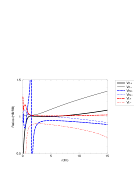
Figure 4: Ratios between the HB and RB components of the TPEP, in configuration space.

In Fig. 4 we plot the ratios of the HB over the RB components of the TPEP. Even though the distance considered is quite large for hadronic interactions, we will show latter in Sec. III that peripheral phase shifts at sufficiently small energies are sensitive to distances as large as 10fm. One can see that the pattern observed in the $1/m$ expansion of our loop functions nos2 reflects more on the isovector (–) channels, but produces deviations smaller than 10% on the isoscalar (+) ones. Note that in the isoscalar central potential it remains below 5% up to 10fm. We omit the ratios of the spin-spin components, which are almost the same as for the corresponding tensor ones. Before commenting further on these results, it is interesting to look how they manifest in the partial wave decomposition.

Figs. 5, 6, and 7 show, for $F$, $G$, and $H$ partial wave channels, respectively, the values of the RB and HB versions of the TPEP multiplied by a common factor $\exp(2\mu r)$, as well as their corresponding ratios. The notation is similar to the one used for phase shifts — for a given total and orbital angular momenta $J$ and $L$, the single channel potentials are identified by $J=L$ waves, while for coupled channels the $2\times 2$ matrix potential has diagonal components $\left[{}^{3}(J-1)_{J},{}^{3}(J+1)_{J}\right]$ and non-diagonal component $\epsilon_{J}$. A chiral TPEP in configuration space has the drawback of being divergent at the origin and, in order to avoid numerical complications while computing phase shifts, we multiply it by a phenomenological regulator,

$$V_{\rm TPEP,\;reg}=\left[1-e^{-cr^{2}}\right]^{4}\,V_{\rm TPEP,\;div}\,,$$ (39)

which is similar to the one used by the Urbana urb and Argonne av14 ; av18 potentials. For the regulator we adopted the value from AV14 av14 , $c=2.0$fm^-2. We will address this question with more details in Sec. V.

Besides the non-diagonal potentials, the ratios clearly show the failure of the HB in describing the correct asymptotic behavior of the TPEP. Such deviations get more dramatic for ${}^{1}F_{3}$, ${}^{3}G_{3}$, ${}^{3}G_{4}$, ${}^{3}G_{5}$, and ${}^{1}H_{5}$ waves (not by accident), being significant already at $r=5$fm. From Fig. 4 it seems strange that differences of the order of 35% turn into $\sim 50-100$% observed for these waves. The reason is that they are channels with total isospin $T=0$, leading to cancelations between isoscalar and isovector components. As an example, for total spin $S=0$ states the tensor and spin-orbit components don’t contribute and the potential is given by

$$V\left[{}^{1}L_{J}\right]=V_{C}^{+}+(4T-3)\,V_{C}^{-}-3\big{[}V_{SS}^{+}+(4T-3)\,V_{SS}^{-}\big{]}=V_{C}^{+}-3\,V_{C}^{-}-3\,\big{[}V_{SS}^{+}-3\,V_{SS}^{-}\big{]}\,.$$ (40)

At $r=6$fm one has, for the RB and HB cases,

$$V\left[{}^{1}L_{J}\right]_{RB}=\big{[}-150.0-3(-78.7)\big{]}-3\big{[}30.1-3(4.28)\big{]}\approx 86.1-51.8\approx 34.3$$ (41)

$$V\left[{}^{1}L_{J}\right]_{HB}=\big{[}-150.7-3(-88.8)\big{]}-3\big{[}30.4-3(3.78)\big{]}\approx 115.7-57.2\approx 58.5$$ (42)

(in units of $10^{-6}$MeV). From Eqs.(41) and (42) one can understand the mechanism that leads to a deviation of roughly 70% in the final result: it comes first from the structure [(isoscalar)-3(isovector)] (which generates more than 30% of deviation from the central component), and is further increased by the sum of central and spin-spin contributions.

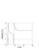
Figure 5: Values of the RB and HB potentials [multiplied by $\exp(2\mu r)$], as well as their ratios, for $F$ waves.

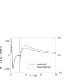
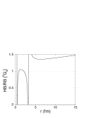
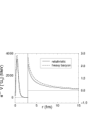
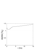
Figure 6: Same as in Fig. 5, for $G$ waves.

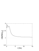
Figure 7: Same as in Fig. 5, for $H$ waves.

III the phase function method

In the calculation of phase shifts we employ the formalism of the variable phase, well studied by a couple of authors in the early sixties calog ; calogrev ; babikov ; babikovrev ; kynch ; coxperl but, surprisingly, not very popular in the nuclear physics community (in the last decade, from the best of our knowledge, only a few works took advantage of this method nalpha ; BRR ; BR ; va04 ). Due to its simplicity, here we outline the main steps to obtain the phase function equation, where its physical interpretation immediately arises. A more detailed description, including scattering with tensor forces, as well as extensions of these ideas to other processes, observables, and kinematics can be found in a review paper by Babikov babikovrev , as well as in the book from Calogero calogrev .

Here we consider the case of a central potential with a regular behavior, i. e., the ones which behave as $r^{-n}$ close to the origin, with $n<2$. The radial Scrödinger equation is written as

$$u^{\prime\prime}_{L}(r)+\big{[}k^{2}-L(L+1)/r^{2}-U(r)\big{]}\,u_{L}(r)=0\,,$$ (43)

with $U(r)=2m_{red}\,V(r)$, and $k=\sqrt{2m_{red}{\cal E}}$, $V(r)$ being the central potential, ${\cal E}$, the energy eigenvalue in the Schödinger equation, $m_{red}$, the reduced mass of the system, and $u_{L}(r)$, the radial wave function.

The basic idea of the phase function method consists in introducing the functions $\delta_{L}(r)$ and $A_{L}(r)$ in such a way that the radial wave function and its derivative are written as

$$u_{L}(r) = A_{L}(r)\big{[}\cos\delta_{L}(r)\,\hat{\jmath}_{L}(kr)-\sin\delta_{L}(r)\,\hat{n}_{L}(kr)\big{]}\,,$$ (44)

$$u^{\prime}_{L}(r) = A_{L}(r)\big{[}\cos\delta_{L}(r)\,\hat{\jmath}^{\prime}_{L}(kr)-\sin\delta_{L}(r)\,\hat{n}^{\prime}_{L}(kr)\big{]}\,,$$ (45)

where $\hat{\jmath}_{L}(x)$ and $\hat{n}_{L}(x)$ are the usual spherical Bessel functions, ${j}_{L}(x)$ and ${n}_{L}(x)$, multiplied by the argument (so called Riccati-Bessel functions). Eq.(44) is just a general parametrization of $u_{L}(r)$, while Eq.(45) imposes the condition

$$A^{\prime}_{L}(r)\big{[}\cos\delta_{L}(r)\,\hat{\jmath}_{L}(kr)-\sin\delta_{L}(r)\,\hat{n}_{L}(kr)\big{]}-\delta^{\prime}_{L}(r)\,A_{L}(r)\big{[}\sin\delta_{L}(r)\,\hat{\jmath}_{L}(kr)+\cos\delta_{L}(r)\,\hat{n}_{L}(kr)\big{]}=0\,.$$ (46)

Substituting Eq.(44) in Eq.(43), using the condition (46), and trigonometric relations we end up with a first order diffential equation for $\delta_{L}(r)$, the “phase function”:

$$\delta^{\prime}_{L}(r)=-\frac{U(r)}{k}\,\Big{[}\cos\delta_{L}(r)\,\hat{\jmath}_{L}(kr)-\sin\delta_{L}(r)\,\hat{n}_{L}(kr)\Big{]}^{2}\,.$$ (47)

Notice that beyond the point where it is assumed to be the range of the potential this function becomes a constant, and the form of Eq.(44) tells us that its value is precisely the phase shift. Furthermore, the condition (46) assures the continuity of the derivative of the wave function at this point. But the phase function means more than that — from Eq.(47) one can easily check that, for a given distance $R$, the quantity $\delta_{L}(R)$ indeed is the phase shift associated to a potential cut at this point, $V(r)\,\theta(R-r)$.

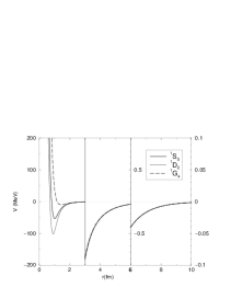
Figure 8: Projections of the AV14 $NN$ potential into ${}^{1}S_{0}$, ${}^{1}D_{2}$, and ${}^{1}G_{4}$ partial waves.

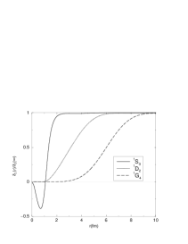
Figure 9: Normalized phase function at $E_{lab}=50$MeV associated to the partial waves from Fig. 9.

This property is particularly interesting to assess the importance of different regions of the potential. For example, in Fig. 9 we show the normalized phase function, $\delta_{L}(r)/\delta_{L}(\infty)$, for nucleon-nucleon scattering in ${}^{1}S_{0}$, ${}^{1}D_{2}$, and ${}^{1}G_{4}$ partial waves, with the laboratory energy at 50MeV. The corresponding potentials, displayed in Fig. 9, are partial wave projections of the Argonne V14 potential av14 . Note that, for ${}^{1}S_{0}$, the repulsive potential in the region $r\lesssim~{}0.8$fm is described by a decrease in the value of the phase function up to a minimum at this point. Beyond that the potential is attractive, resulting in positive increments to $\delta_{L}(r)$. For the other waves, the phase function also shows nicely the effect of the centrifugal barrier which, for sufficiently large $L$ and small energy, supress the dependence of the phase on the short range structure of the potential. In the next section we take advantage of this feature to determine the ranges of relevance when extracting the phase shifts.

IV LECs and phase shifts

In this section we present our studies for peripheral phase shifts. The calculations are performed in configuration space using the phase function method described in the previous section, which is fully equivalent to the Schrödinger equation. The final $NN$ potential is the sum of TPEP and OPEP and we disregard the exchange of three or more pions, which are much more weaker and smaller in range egm04-2 ; Kaiser4 ; joel . We use the Fourier transform of the same charge-dependent OPE for neutron-proton scattering used by Entem and Machleidt EM ,

$$V_{OPE}=-V_{\pi}(\mu_{\pi^{0}})+(-1)^{T+1}\,2\,V_{\pi}(\mu_{\pi^{\pm}})\,,$$ (48)

with $\mu_{\pi^{0}}=134.9766$ MeV, $\mu_{\pi^{\pm}}=139.5702$ MeV, and the function $V_{\pi}(\mu)$ defined as

$$V_{\pi}(\mu)=\frac{\mu^{2}g_{A}^{2}}{4f_{\pi}^{2}}\,\frac{e^{-\mu r}}{\mu r}\left\{\left[1+\frac{3}{\mu r}+\frac{3}{(\mu r)^{2}}\right]S_{12}+{\mbox{\boldmath$\sigma$}}^{(1)}\cdot{\mbox{\boldmath$\sigma$}}^{(2)}\right\}\,,$$ (49)

where $S_{12}$ is the usual tensor operator in configuration space. This is the same charge-dependent OPEP used in Refs. nij93 ; av18 , provided we set the scaling mass $m_{s}$ and the couplings as

$$m_{s}=\mu_{\pi^{\pm}}\,,\qquad\qquad\quad f_{pp}=-f_{nn}=\frac{1}{\sqrt{4\pi}}\,\frac{\mu_{\pi^{\pm}}\,g_{A}}{2f_{\pi}}\,.$$ (50)

For our TPEP we use the average nucleon and pion mass from the AV18 potential av18 , $m=938.9190$ MeV and $\mu=138.0363$ MeV. The remaining constants besides the LECs are $\hbar c=197.3270$ MeV.fm, $f_{\pi}=92.4$ MeV, and $g_{A}=1.3187$, the latter being higher than the experimental value in order to accommodate the Goldberger-Treiman discrepancy. In this work we did not consider the quadratic spin-orbit term, given by Eq.(26). Its effect on the phase shifts is expected to be insignificant for the waves we are considering as we could estimate, for instance, by switching on and off the $L^{2}$ and $(L\cdot S)^{2}$ components of the Argonne V14 potential and comparing the results.

Table 3: Values for the dimension two ($c_{i}$) and three ($\bar{d}_{i}$) LECs considered in this work, given respectively in GeV^-1 and GeV^-2.

LEC	Ref. moj98	Ref. fms98 (fit 1)	Ref. butik	Ref. nij03	Ref. EM
$c_{1}$	-0.94	-1.23	-0.81	-0.76	-0.81
$c_{2}$	3.20	3.28	8.43	3.20	3.28
$c_{3}$	-5.40	-5.94	-4.70	-4.78	-3.40
$c_{4}$	3.47	3.47	3.40	3.96	3.40
$\bar{d}_{1}+\bar{d}_{2}$	2.40	3.06	3.06	2.40	3.06
$\bar{d}_{3}$	-2.80	-3.27	-3.27	-2.80	-3.27
$\bar{d}_{5}$	1.40	0.45	0.45	1.40	0.45
$\bar{d}_{14}-\bar{d}_{15}$	-6.10	-5.65	-5.65	-6.10	-5.65

Concerning the LECs, in table 3 we display their values from five different studies. The first column was extracted from a work from Mojžiš moj98 where he presented the first complete $O(q^{3})$ expressions for $\pi N$ scattering amplitude and pinned down the LECs using the Karlsruhe-Helsinki kochpiet threshold parameters in combination with the pion-nucleon $\sigma$ term. The second column was determined by Fettes et.al. fms98 through a direct fit to $S$- and $P$- wave $\pi N$ phase shifts between 40 and 100 MeV pion lab momentum, using the Karlsruhe partial wave analysis ka84 (fit 1). The third column shows the results from Büttiker and Meißner butik , where the $\pi N$ amplitude was reconstructed inside the Mandelstam triangle via dispersion relations, then the LECs were obtained through a fit to this amplitude, in two different points (because their results for the dimension three LECs were not consistent, we adopt here the same values from the second column). These three works rely on old Karlsruhe dispersion analyses, which have presumably some inconsistent data included pinlett . Different from them, the dimension two LECs on the fourth column were determined by the Nijmegen group nij03 from their new partial wave analyses of 5109 proton-proton and 4786 neutron-proton scattering data below 500 MeV. As the dimension three LECs were not considered in their work, for this set we adopted the same values from Mojžiš. Finally, on the last column we have the values used by Entem and Machleidt in their calculations of neutron-proton phase shifts EM .

In the calculation of phase shifts we use the familiar nuclear-bar convention dbar , where the coupled $S$ matrix with total angular momentum $J$ is parametrized as

$$S_{J}=\pmatrix{e^{2i\delta_{J-1}}\,\cos 2\epsilon_{J}&i\,e^{2i(\delta_{J-1}+\delta_{J+1})}\,\sin 2\epsilon_{J}\cr i\,e^{2i(\delta_{J-1}+\delta_{J+1})}\,\sin 2\epsilon_{J}&e^{2i\delta_{J+1}}\,\cos 2\epsilon_{J}}\,.$$ (51)

Before addressing their dependence on different sets of LECs it is interesting to take advantage of the phase function formalism (Sec. III) to identify the most important ranges of the potential in the determination of these quantities. In Figs. 10, 11, and 12 we plot the distances where the phase function $\delta_{L}(r)$ reaches 10%, 20%, and so on, up to 90%, of the final value, $\delta_{L}(\infty)$, as functions of the laboratory energy, $E_{\rm LAB}$. As in Sec. II, we use here a potential with LECs from Entem and Machleidt (last column of table 3) and similar curves are obtained for the other sets. These figures show, quantitatively, the sensitivity of phase shifts on large distances at sufficiently low energies. We also notice that the range, delimited by the points where the phase function reaches 10% and 90% of the final value, gets narrower and closer to the inner region of the potential as we go higher in energies, but not smaller than 1fm (1.5fm) for $F$ ($G$ and $H$) waves, a clear manifestation of the centrifugal barrier.

Figure 10: Distances, for $F$ waves, where the phase shift (or mixing parameter) achieves $X$% of its value, as functions of the laboratory energy. The curves correspond, from bottom to top, to $X=$10, 20, $\cdots$, 90, respectively.

Figure 11: Same as Fig. 10, for $G$ waves.

Figure 12: Same as Fig. 10, for $H$ waves.

Figs. 13, 14, and 15 show, respectively, the phase shifts associated to $F$, $G$, and $H$ waves, as functions of the laboratory energy. The dotted lines correspond to LECs from Mojžiš (column 1), dot-dashed, from Fettes et.al. (column 2), dashed, from Büttiker and Meißner (column 3), solid, from the Nijmegen group (column 4), and thick solid, from Entem and Machleidt (column 5). The dark and light lines represent, respectively, calculations using the RB and HB formalism. As it is clear, from $NN$ scattering phase shifts one cannot observe any significant difference between RB and HB results — despite the contrast between them, shown in Sec. II.4, in $NN$ scattering one also has to add the OPEP, which gives a large contribution and makes such discrepancies harder to observe. Exeptions are the $F$ wave results using the LECs from Fettes et.al., but their predictions are not very close from what one should expect.

It is noticeable the large variations of the phase shifts with different sets of LECs, predominantly due to $c_{3}$ (the leading order term of the nucleon axial polarizability tarer ). As pointed out by Entem and Machleidt EM , consistency with the experimental analysis (Figs. 16, 17, and 18) favors a smaller value for this particular LEC, $c_{3}\sim-3.4$. We will discuss this issue later in Sec. V.

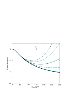
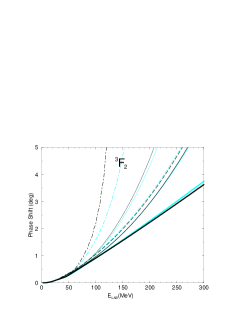
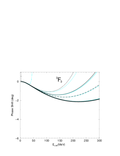
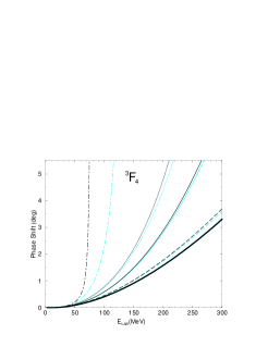
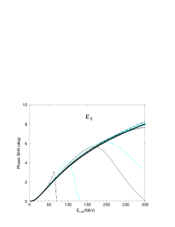
Figure 13: Phase shifts and mixing parameter for $F$ waves, as functions of the laboratory energy. The dotted, dot-dashed, dashed, solid, and thick-solid lines correspond to LECs from table 3: columns 1, 2, 3, 4, and 5, respectively. The dark curves are results from the RB formalism, while the light ones, from the HB expressions.

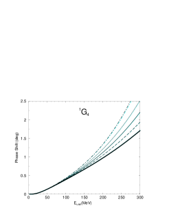
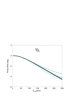
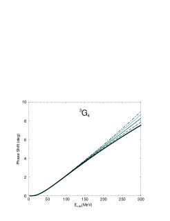
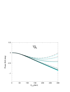
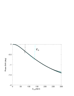
Figure 14: Phase shifts and mixing parameter for $G$ waves, as functions of the laboratory energy. Notation is the same used in Fig. 13.

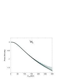
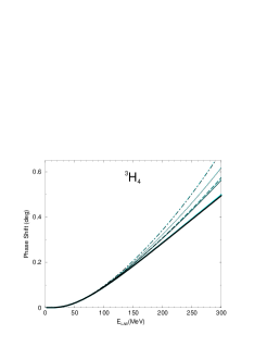
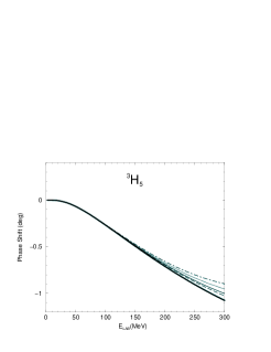
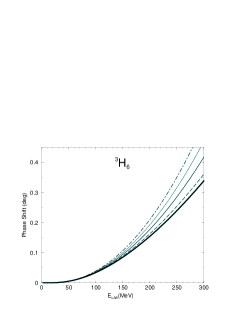
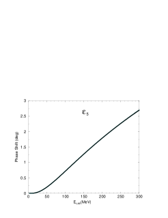
Figure 15: Phase shifts and mixing parameter for $H$ waves, as functions of the laboratory energy. Notation is the same used in Fig. 13.

In Figs. 16, 17, and 18 we compare the phase shifts associated to the LECs from column 4 (dark, dashed curves) and column 5 (dark, solid lines) of table 3 with the Nijmegen partial wave analysis (circled line) nnonline . It is important to emphasize that, in Refs. nij99 ; nij03 , the Nijmegen group employ the TPEP up to $O(q^{3})$ to determine the dimension two LECs $c_{1}$, $c_{3}$, and $c_{4}$. For this reason, we also plot the phase shifts using the TPEP up to this order with their LECs, indicated by the (light) dot-dashed curves.

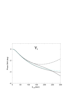
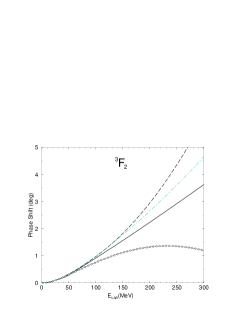
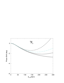
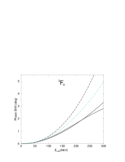
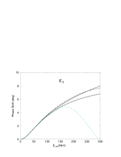
Figure 16: Phase shifts and mixing parameter for $F$ waves, as functions of the laboratory energy, compared with the Nijmegen partial wave analysis (circled line) nnonline . The solid and dashed (dark) lines correspond to OPE plus TPE up to $O(q^{4})$ using, respectively, the LECs from Nijmegen (column 4) and Entem and Machleidt (column 5), while the dot-dashed (light) curves are results from OPE+TPE up to $O(q^{3})$, using the LECs from Nijmegen.

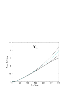
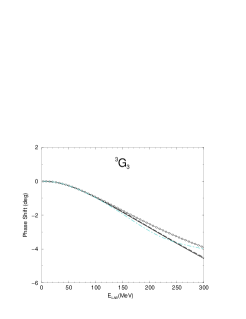
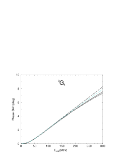
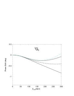
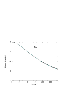
Figure 17: Phase shifts and mixing parameter for $G$ waves, as a function of the laboratory energy. Notation is the same used in Fig. 16.

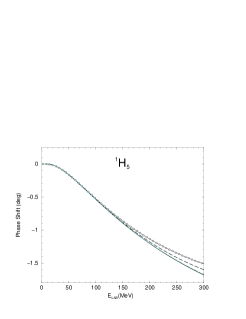
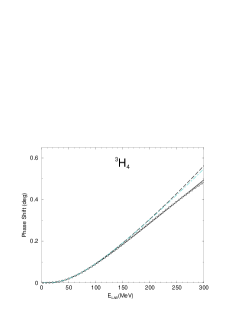
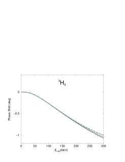
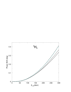
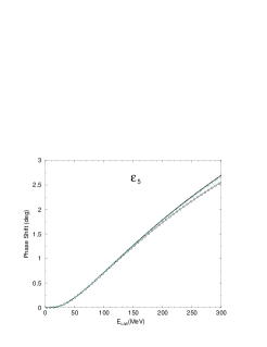
Figure 18: Phase shifts and mixing parameter for $H$ waves (as a function of the laboratory energy). Notation is the same used in Fig. 16.

V comments and summary

As mentioned in Sec. II.4, the calculation of phase shifts requires the regularization of the potential near the origin and, as a consequence, makes our calculation dependent on the value of the regulator. This procedure is analogous to, in momentum space, introduce a cutoff in the dynamical equation, and seems to be unavoidable when dealing with two or more nucleon systems. There are, though, attempts to reformulate the problem using dimensional regularization PAH or variants fuchs ; goity in the literature. One should emphasize that even if the chiral potential is finite in momentum space, its representation in configuration space shows a divergence at the origin of the type $r^{-n}$, where $n$ is some integer. It simply maps the fact that a chiral potential has a limited region of applicability, increasing as a polinomial in $q$ (in contrast, for instance, with phenomenological one-boson exchange potentials). The advantage to work in configuration space is that statements about ranges and nucleon sizes can be made more transparently, and also it is more suitable to be extended to few body calculations for nuclei up to $A=10$, e.g., by means of the Variational or Green Function Monte Carlo techniques gfmc .

We introduced a regulator given by Eq.(39), with $c=2.0$fm^-2, in our calculations. In principle there is not a real compelling justification to use such a value. With higher values, however, the phase shifts using the LECs from Fettes et.al., or from Mojžiš, become even more unrealistic. For lower values the situation interchanges, as ilustrated in Fig. 20, but at the expense of large modifications in the strength of the potential. For example, using $c=1.0\mbox{\rm fm}^{-2}$ one has a reduction of almost half of the “bare” value of the potential at $r=1.4$fm. With $c=2.0\mbox{\rm fm}^{-2}$ at the same point, it reduces roughly 8%. From the same figure we see that, even with this regulator, the sets with larger absolute values of $c_{3}$ are still far from PWA results (Figs. 16–18). There might be two explanations for this to happen. One, that $F$ waves are not peripheric enough to avoid the dependence on short distances of the potential, but we check that similar behavior holds for ${}^{1}G_{4}$ wave as well. Also, one can rule out this option by calculating the phase shifts in Born approximation, as shown in Fig. 20, where there is no need to regulate the potential near the origin.

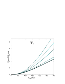
Figure 19: ${}^{3}F_{4}$ phase shifts, using $c=1.0\mbox{\rm fm}^{-2}$ for the regulator. Notation is the same used in Fig. 13.

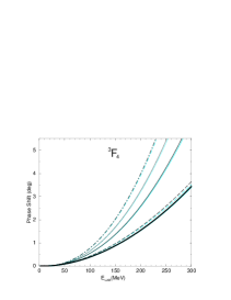
Figure 20: Born approximation for ${}^{3}F_{4}$ phase shifts. Notation is the same used in Fig. 13.

The other possible explanation rely on EFT ideas to deal with divergences in the dynamical equation, implemented by the introduction of a cutoff. To be consistent, the same cutoff should also regularize loop integrals for the irreducible two-nucleon diagrams that constitute the kernel (or the potential) of the dynamical equation . This procedure can weaken the contribution of pion loops at short and intermediate distances, enough to allow larger absolute values for $c_{3}$ egm04-1 . We do not address this alternative in the present work, as we keep the possibility of renormalize the dynamical equation by other means, as the ones mentioned before.

A further remark on the regulator is that our calculations, using the same LECs from Entem and Machleidt, are not very sensitive to its variations in the range $1.0\mbox{\rm fm}^{-2}\leq c\leq 3.0\mbox{\rm fm}^{-2}$, except for ${}^{3}F_{3}$ and ${}^{3}F_{4}$ waves. Using $c=2.5\mbox{\rm fm}^{-2}$, we have all of our results very close to theirs EM .

One comment on Figs. 16–18 is in order. We can see that using the LECs from the Nijmegen group on the expressions of the $O(q^{4})$ TPEP does not give a good description of results from PWA, but this procedure does not make sense, as these LECs were determined using a potential to $O(q^{3})$ nij99 ; nij03 . It is well known that the LECs pinned down by any particular process depend on the order one is working on. Formally the difference between using an $O(q^{3})$ and $O(q^{4})$ TPEP should be of higher order, but in practice it is sizeable (see, for instance, the $\pi N$ scattering analysis from Ref. fet04 ). We can check that the too strong attraction, which arises if one uses the LECs from the Nijmegen group in the $O(q^{4})$ potential (Nij⁴), is actually not that attractive if one considers it up to $O(q^{3})$ (Nij³), bringing their phase shifts closer to the ones from PWA. Fig. 21 ilustrates this point for ${}^{1}F_{3}$ wave. The thick-solid curve is the potential using the LECs from Entem and Machleidt, while the dashed and solid curves are the Nij³ and Nij⁴ potentials, respectively. For comparison purposes, we also include the OPEP (light, dotted curve) and the phenomenological Reid 93 potential nnonline ; reid93 (dot-dashed curve).

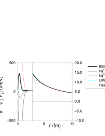
Figure 21: ${}^{1}F_{3}$ potential. Notation is given in the text.

From this figure and what we discussed above one can say that the argument given by Entem and Machleidt EM ; EMach-com , that the LEC $c_{3}$ from the Nijmegen group leads to a much stronger potential as a result of a cutoff in the potential at 1.4fm or 1.6fm (and set to zero until the origin) could have some meaning only if such a value were extracted from an $O(q^{4})$ TPEP. Evidently this is not the case, primarily because the energy-dependent boundary conditions of Nijmegen PWA at $r=1.6$fm does not mean that the potential is zero inside this range. Besides that, the Nij³ potential shows a repulsion beyond $r\sim 1.2$fm, as can be seen in Fig. 21. The (now, not too large) disagreement of Nij³ must have other explanations. From our point of view, the reason is that the LECs are parameters in the TPEP beyond 1.6fm which are determined when the fit to scattering data gives the best $\chi^{2}$ with a minimum number of boundary conditions. This involves sums also over lower partial waves, where the nonperturbative aspect of the nucleon-nucleon interaction is more pronounced. Therefore, the way short distances are parametrized can contaminate the actual value of these LECs, contributing as a systematic error. Moreover, contact terms can start contributing at $O(q^{5})$ or $O(q^{6})$ to $F$ waves, which can change the the behavior of phase shifts even at not so large energies comun . When fitting to data, these terms are inherently taken into account.

To summarize, in this work we address the discrepancies we found when comparing our $1/m$ expanded results with the expressions from the HB formalism. It forced us to revise not only our $1/m$ expansions, but also our two loop diagrams, and now we have a better understanding about the origin of the remaining discrepant terms. There are, however, two terms in the central isovector component, originated from two loop calculations, which could not be understood. It will be necessary to solve them if claims for higher order calculations of the chiral $NN$ potential becomes imminent. In a second stage we calculate the phase shifts for peripheral waves ($F$, $G$, and $H$), where short distances are supposed to play a minor role. This was shown in Figs. 10–12, where the ranges relevant to phase shifts where determined using the method of the phase function. Our results for phase shifts reveals that, due to the overwhelming contribution of the OPEP, any difference between the RB- and HB- TPEP is barely noticed. It is possible that these differences might be relevant in processes where the OPEP is cancelled, and the dominant tail of the interaction, given by the TPEP, for instance, in low-energy peripheral scattering of nucleons off isoscalar targets nisoscat . A more relevant question, there are large variations of the phase shifts with the existing values of LECs, predominantly due to $c_{3}$, which dictates the strength of the attraction of the potential. Consistency with PWA favors smaller values, in magnitude, than the existent ones in the literature. There are, however, conceptual details mentioned before which prevent, at the moment, to constrain these LECs with a satisfactory precision. They should be well understood and quantified if one aims to extract values with good precision from $NN$ scattering.

References

- (1) S. Weinberg, Physica 96 A, 327 (1979).
- (2) S. L. Adler and R. F. Dashen, Current Algebras and Applications to Particle Physics, Benjamin, New York (1968); V. de Alfaro, S. Fubini, G. Furlan, and C. Rosseti, Currents in Hadron Physics, North-Holland, Amsterdam (1973).
- (3) J. Gasser and H. Leutwyler, Ann. Phys. 158, 142 (1984); Nucl. Phys. B250, 465 (1985).
- (4) G. Ecker, Prog. Part. Nucl. Phys. 35, 1 (1995).
- (5) V. Bernard, N. Kaiser, and Ulf-G. Meißner, Int. J. Mod. Phys. E 4, 193 (1995).
- (6) S. Scherer, Advances in Nuclear Physics, Vol. 27, ed. J. W. Negele and E. W. Vogt (Kluwer Academic/Plenum Publishers, New York, 2002).
- (7) J. Gasser, M. E. Sainio, and A. Švarc, Nucl. Phys. B307, 779 (1988).
- (8) E. Jenkins and A. V. Manohar, Phys. Lett. 255, 558 (1991).
- (9) T. Becher and H. Leutwyler, Eur. Phys. Journal C 9, 643 (1999).
- (10) T. Becher and H. Leutwyler, JHEP 106, 17 (2001).
- (11) H.-B. Tang, hep-ph/9607436; P. J. Ellis and H.-B. Tang, Phys. Rev. C 57, 3356 (1998); K. Torikoshi and P. Ellis, Phys. Rev. C 67, 015208 (2003).
- (12) T. Fuchs, J. Gegelia, G. Japaridze, and S. Scherer, Phys.Rev. D 68, 056005 (2003); M. R. Schindler, J. Gegelia, and S. Scherer, Phys. Lett. B 586, 258 (2004); Nucl. Phys. B682, 367 (2004).
- (13) M. F. Lutz and E. E. Kolomeitsev, Nucl. Phys. A700, 193 (2002).
- (14) J.L. Goity, D. Lehmann, G. Prezeau, and J. Saez, Phys. Lett. B 504, 21-27 (2001); D. Lehmann, G. Prezeau, Phys. Rev. D 65, 016001 (2002).
- (15) R. Higa and M.R. Robilotta, Phys. Rev. C 68, 024004 (2003).
- (16) R. Higa, M. R. Robilotta, and C. A. da Rocha, Phys. Rev. C 69, 034009 (2004).
- (17) D. R. Entem and R. Machleidt, Phys. Rev. C 66, 014002 (2002).
- (18) V. Bernard, N. Kaiser, and U.-G. Meißner, Nucl. Phys. A615, 483 (1997).
- (19) G. Ecker, J. Gasser, H. Leutwyler, A. Pich, and E. de Rafael, Phys. Lett. B 223, 425 (1989); G. Ecker, J. Gasser, A. Pich, and E. de Rafael, Nucl. Phys. B321, 311 (1989).
- (20) R. Machleidt, K. Holinde, and Ch. Elster, Phys. Rep. C 149, 1 (1987).
- (21) M. Mojžiš, Eur. Phys. J. C 2, 181 (1998).
- (22) A. Datta and S. Paksava, Phys. Rev. D 56, 4322 (1997).
- (23) N. Fettes, U.-G. Meißner, and S. Steininger, Nucl. Phys. A640, 199 (1998).
- (24) P. Büttiker and U.-G. Meißner, Nucl. Phys. A668, 97 (2000).
- (25) E. Epelbaum, A. Nogga, W. Glöckle, H. Kamada, U.-G. Meißner, and H. Witala, Eur. Phys. J. A 15 (2002), 543.
- (26) R. Koch and E. Pietarinen, Nucl. Phys. A336, 331 (1980).
- (27) R. Koch and M. Hutt, Z. Phys. C 19, 119 (1983); R. Koch, Z. Phys. C 29, 597 (1985); Nucl. Phys. A448, 707 (1986).
- (28) M. C. M. Rentmeester, R. G. E. Timmermans, J. L. Friar, and J. J. de Swart, Phys. Rev. Lett. 82, 4992 (1999).
- (29) M. C. M. Rentmeester, R. G. E. Timmermans, and J. J. de Swart, Phys. Rev. C 67, 044001 (2003).
- (30) D. R. Entem e R. Machleidt, nucl-th/0303017 (2003).
- (31) S. Weinberg, Phys. Lett. B 251, 288 (1990); Nucl. Phys. B363, 3 (1991).
- (32) S. R. Beane, P. F. Bedaque, W. C. Haxton, D. R. Phillips, and M. J. Savage, in At the frontier of particle physics, ed. M. Shifman, Vol. 1, pp. 133 [arXiv: nucl-th/0008064].
- (33) T.-S. Park, K. Kubodera, D.-P. Min, and M. Rho, Nucl.Phys. A 646, 83 (1999).
- (34) U. van Kolck, Prog. Part. Nucl. Phys. 43, 337 (1999).
- (35) C. Ordoñez and U. van Kolck, Phys. Rev. Lett. 72, 1982 (1994); C. Ordoñez, L. Ray, and U. van Kolck, Phys. Rev. C 53, 2086 (1996).
- (36) G. P. Lepage, arXiv: nucl-th/9706029.
- (37) E. Epelbaum, W. Glöckle, and Ulf-G. Meißner, Nucl. Phys. A637, 107 (1998); ibid. A671, 295 (2000).
- (38) E. Epelbaum, W. Glöckle, and Ulf-G. Meißner, Eur. Phys. J. A 19, 125 (2004).
- (39) E. Epelbaum, W. Glöckle, and Ulf-G. Meißner, Eur. Phys. J. A 19, 401 (2004); arXiv: nucl-th/0405048.
- (40) M. C. Birse, J. A. McGovern, and K. G. Richardson, Phys. Lett. B 464, 169 (1999).
- (41) T. D. Cohen, B. A. Gelman, and U. van Kolck, Phys.Lett. B 588, 57 (2004).
- (42) M. P. Valderrama and E. R. Arriola, Phys. Lett. B 580, 149 (2004); arXiv: nucl-th/0407113.
- (43) D. B. Kaplan, M. J. Savage, and M. B. Wise, Nucl. Phys. B478, 629 (1996); Phys. Lett. B 424, 390 (1998); Nucl. Phys. B534, 329 (1998).
- (44) S. Fleming, T. Mehen, and I. W. Stewart, Nucl. Phys. A677, 313 (2000); Phys. Rev. C 61, 044005 (2000).
- (45) S. R. Beane, P. F. Bedaque, M. J. Savage, and U. van Kolck, Nucl. Phys. A700, 377 (2002); P. F. Bedaque and U. van Kolck, Ann. Rev. Nucl. Part. Sci. 52, 339 (2002).
- (46) J. Gegelia, J. Phys. G 25, 1681 (1999); Eur.Phys.J. A 19, 355 (2004); J. Gegelia and G. Japaridze, Phys. Lett. B 517, 476 (2001); J. Gegelia and S. Scherer, arXiv: nucl-th/0403052; D. Djukanovic, M.R. Schindler, J. Gegelia, and S. Scherer, arXiv: hep-ph/0407170.
- (47) J.-F. Yang, arXiv: nucl-th/0407090; J.-F. Yang and J.-H. Huang, arXiv: nucl-th/0409023.
- (48) N. Kaiser, R. Brockman, and W. Weise, Nucl. Phys. A625, 758 (1997).
- (49) N. Kaiser, Phys. Rev. C 64, 057001 (2001).
- (50) N. Kaiser, Phys. Rev. C 65, 017001 (2001).
- (51) J-L. Ballot, C. A. da Rocha, and M. R. Robilotta, Phys. Rev. C 57, 1574 (1998).
- (52) J-L. Ballot and M. R. Robilotta, J. Phys. G 20, 1599 (1994); Z. Phys. A 355, 81 (1996).
- (53) S. A. Coon and J. L. Friar, Phys. Rev. C 34, 1060 (1986).
- (54) J. L. Friar, Phys. Rev. C 60, 034002 (1999).
- (55) G. Ramalho, A. Arriaga, and M. T. Peña, Phys. Rev. C 60, 047001 (1999); Phys. Rev. C 65, 034008 (2002).
- (56) R. Blankenbecler and R. Sugar, Phys. Rev. 142, 1051 (1966).
- (57) S. J. Wallace and V. B. Mandelzweig, Nucl. Phys. A503, 673 (1989).
- (58) F. Gross, Phys. Rev. 186, 1448 (1969); F. Gross, J. W. Van Orden, and K. Holinde, Phys. Rev. C 45, 2094 (1992).
- (59) G. Höhler, group I, vol.9, subvol.b, part 2 de Landölt-Bornstein Numerical data and Functional Relationships in Science and Technology, ed. H.Schopper (1983); G. Höhler, H. P. Jacob e R. Strauss, Nucl. Phys. B39, 237 (1972).
- (60) M. R. Robilotta and C.A. da Rocha, Phys. Rev. C 49, 1818 (1994); Phys. Rev. C 52, 531 (1995); Nucl. Phys. A615,391 (1997).
- (61) Work in progress.
- (62) I. E. Lagaris and V. R. Pandharipande, Nucl. Phys. A359, 331 (1981).
- (63) R. B. Wiringa, R. A. Smith, and T. L. Ainsworth, Phys. Rev. C 29, 1207 (1984).
- (64) R. B. Wiringa, V. G. J. Stoks, and R. Schiavilla, Phys. Rev. C 51, 38 (1995).
- (65) F. Calogero, Nuovo Cimento 27, 261 (1963).
- (66) F. Calogero, Variable Phase Approach to Potential Scattering (Academic Press, New York, 1967).
- (67) V. V. Babikov, Sov. Phys.-Usp. 92, 271 (1967).
- (68) V. V. Babikov, Sov. J. Nucl. Phys. 1, 261 (1965).
- (69) G. J. Kynch, Proc. Phys. Soc. A 65 (London), 83; ibid., 94 (1952).
- (70) J. R. Cox and A. Perlmutter, Nuovo Cimento 37, 76 (1965).
- (71) L. A. Barreiro, R. Higa, C. L. Lima, and M. R. Robilotta, Phys. Rev. C 57, 2142 (1998); R. Higa and M. R. Robilotta, arXiv: nucl-th/9908062 (1999).
- (72) N. Kaiser, Phys. Rev. C 61, 014003 (2000); ibid C 62, 024001 (2000); ibid C 63, 044010 (2001).
- (73) J. C. Pupin and M. R. Robilotta, Phys. Rev. C 60, 014003 (1999).
- (74) V. G. J. Stoks, R. A. M. Klomp, M. C. M. Rentmeester, and J. J. de Swart, Phys. Rev. C 48, 792 (1993).
- (75) Proceedings of the Seventh International Symposium on Meson-Nucleon Physics and the Structure of the Nucleon, published in Newsletter 13, 1–398 (1997).
- (76) SAID on-line program, R. A. Arndt et. al., http://gwdac.phys.gwu.edu.
- (77) R. Tarrach and M. Ericson, Nucl. Phys. A294, 417 (1978).
- (78) H. P. Stapp, T. J. Ypsilantis, and N. Metropolis, Phys. Rev. 105, 302 (1957).
- (79) Nijmegen on-line program, http://nn-online.org.
- (80) D. R. Phillips, I. R. Afnan, and A. G. Henry-Edwards, Phys. Rev. C 61, 044002 (2000).
- (81) R. B. Wiringa, S. C. Pieper, J. Carlson, and V. R. Pandharipande, Phys. Rev. C 62, 014001 (2000); S. C. Pieper, K. Varga, and R. B. Wiringa, Phys. Rev. C 66, 044310 (2002).
- (82) V. G. J. Stoks, R. A. M. Klomp, C. P. F. Terheggen, and J. J. de Swart, Phys. Rev. C 49, 2950 (1993).
- (83) N. Fettes and U.-G. Meißner, Nucl.Phys. A676, 311 (2000).
- (84) L. A. Barreiro, R. Higa, C. L. Lima, and M. R. Robilotta, Phys. Rev. C 57, 2142 (1998); R. Higa and M. R. Robilotta, arXiv: nucl-th/9908062 (1999); R. Higa, in International Workshop on Hadron Physics 2000, editors F. S. Navarra, M. R. Robilotta, and G. Krein, World Scientific.
- (85) E. Epelbaum, private communication.