Signature of Granular Structures by Single-Event Intensity Interferometry

Abstract

The observation of a granular structure in high-energy heavy-ion collisions can be used as a signature for the quark-gluon plasma phase transition, if the phase transition is first order in nature. We propose methods to detect a granular structure by the single-event intensity interferometry. We find that the correlation function from a chaotic source of granular droplets exhibits large fluctuations, with maxima and minima at relative momenta which depend on the relative coordinates of the droplet centers. The presence of this type of maxima and minima of a single-event correlation function at many relative momenta is a signature for a granular structure and a first-order QCD phase transition. We further observe that the Fourier transform of the correlation function of a granular structure exhibits maxima at the relative spatial coordinates of the droplet centers, which can provide another signature of the granular structure.

I Introduction and Summary

Recently, much progress has been made in the experimental search for the quark-gluon plasma Gyu04 ; Rik04 . The occurrence of jet-quenching and collective flow suggests the presence of a very dense matter produced in high-energy heavy-ion collisions Gyu04 ; Rik04 . A very important question is whether the produced dense matter is a quark-gluon plasma. If it is a quark-gluon plasma, it will undergo a phase transition from the quark-gluon plasma phase to the hadronic phase. It is of great interest to search for the signature for the phase transition of the quark-gluon plasma.

The signature for the phase transition depends sensitively on the order of the transition. Previously, Witten and many other workers noted that a granular structure of droplets occurs in a first-order QCD phase transition, and the observation of the granular structure can be used as a signature for a first-order QCD phase transition Wit84 -Ran04a . In a recent spinodal analysis, Randrup found that the spinodal instability has a high degree of amplification and the instability of the most rapidly amplified wavelengths grow predominantly, leading to spinodal (granular) density patterns that may indeed be used as a diagnostic tool for a first-order QCD phase transition Ran04 . Assuming that the granular particles are arranged in regular rapidity intervals in momentum space, Randrup studied methods to identify the associated momentum clumping using N-particle momentum correlations Ran04a .

We would like to study the granular source in configuration space. Among the many different ways to study a quark-gluon plasma, intensity interferometry (HBT interferometry) is the best experimental tool to examine the space-time density distribution of the produced matter Won94 -Bro04a . It can be utilized to study the granular structure that occurs in a first-order phase transition of the plasma.

It should be pointed out that without a careful study of the phase-transition dynamics and post-transition evolution, it is not known at present how much the granular density pattern of the phase transition will remain and become detectable by HBT interferometry. It also remains a subject of current research how early a post-transition configuration the HBT interferometry really detects, as it was shown by quantum treatments of the multiple scattering process and the collective flow that HBT interferometry measures the density distribution at a configuration earlier than the thermal freeze-out configuration Won03 ; Won04 ; Zha04a ; Kap04 . To continue our progress in the search for the phase transition of a quark-gluon plasma, it is reasonable to start with the working hypothesis that the density fluctuations that occur during a first-order phase transition are so large that some remnants of the granular droplet distribution remain after the post-transition evolution, and these remnants form an initial chaotic source of granular droplets. The assumed chaoticity of the particle source then leads to the result that the correlation function of two identical bosons in HBT interferometry contains information on the space-time density of the source. A granular density distribution of the emitting chaotic source then distinguishes itself from other density distributions and should reveal its characteristics in HBT interferometry.

Suggestions to examine the granular structure in connection with the phase transition of the quark-gluon plasma have been presented previously Wit84 -Ran04a . Recent high-energy heavy-ion measurements give a ratio of $R_{\rm out}/R_{\rm side}\sim 1$ PHE02 ; STA01 , which is contrary to most theoretical expectations Pra03 -Mol04 . A granular emitting source of droplets was proposed to explain this HBT interferometry puzzle Zha04 . The suggestion was based on the observation that in the hydrodynamical model Ris96 , the particle emission time scales with the radius of the droplet. Particles will be emitted earlier if the radius of the droplet is smaller, as in a source of many droplets. An earlier emission time will lead to a smaller extracted HBT radius $R_{\rm out}$. On the other hand, $R_{\rm side}$ depends on the distribution of droplet centers and is relatively independent of the droplet size. It increases with an increase in the width of the droplet center distribution and the collective-expansion velocity of the droplets. As a result, the value of $R_{\rm out}$ can lie close to $R_{\rm side}$ for a granular quark-gluon plasma source. A direct investigation on the granular density structure of the emitting source is, however, needed to confirm the occurrence of a granular structure in high-energy heavy-ion collisions.

Previously, Pratt $et~{}al.$ Pra92 studied the granular density structure in HBT interferometry by considering pairs of identical bosons in a distributed source in which the centers of the droplets are distributed according to a spherical Gaussian distribution with a standard deviation $R_{0}/\sqrt{2}$. They calculated the correlation function $C(|{\bf q}|)$ for a pair of identical bosons of relative momentum ${\bf q}$ from such a distributed source with $R_{0}=4$ fm. They found that there are differences in the magnitudes of the correlation function $C(|{\bf q}|)$ at $|{\bf q}|$ greater than about 80 MeV/c in a granular structure. They also found that the correlation functions are relatively smooth functions of $|{\bf q}|$ even for small numbers of droplets (2 and 4).

The source considered by Pratt $et~{}al.$ in Ref. Pra92 corresponds to a source in which the centers of the droplets have been distributed first and identical bosons are then subsequently examined from such a distributed source. In actual dynamics with droplet formation in a first-order phase transition Wit84 , one envisages the formation of localized droplets in each single event following the phase transition, and particles are emitted and evolve from these localized granular droplets. Although there can be a distribution of the centers of the localized droplets over many different heavy-ion collision events (of similar other global characteristics), the centers of the droplets in each single collision event can be localized.

Noting that the centers of the droplets in each single event can be localized in space and time, we would like to consider a different way to study the granular structure in HBT interferometry. We propose experiments to look at HBT interferometry for each event individually, to study its associated density distribution. There are many advantages in the single-event HBT interferometry, if it can be carried out with sufficient accuracy. First, the granular structure is the result of a large fluctuation of the density distribution in space and time as it undergoes a first-order phase transition. The large fluctuation of the density in space and time is encoded into its corresponding Fourier transform, whose absolute square gives the correlation function of identical bosons. By considering the correlation function of all pairs of identical bosons from this single event, one can obtain pertinent information on the density distribution of the event. One can even invert the correlation function with an inverse Fourier transform to obtain an integral equation for the source density distribution of the event. Secondly, as a result of the large fluctuation in the dynamics of a first-order phase-transition, the granular structure of one event will be quite different from the granular structure of another event, even though many other global characteristics can be very similar. By examining the space-time structure of each event individually one can study the large fluctuation of different events in the phase transition, which is another characteristic of a first-order phase transition. In other words, there are both large fluctuations in a single event as well as large fluctuations among different events in a first-order QCD phase transition. Finally, any averaging over a set of collision events to obtain an average correlation function, as in the use of identical boson pairs from different collision events in a ‘multi-event’ analysis or in considering bosons from a ‘distributed source’, will wash out the large fluctuations in the single-event correlation function. As a consequence, the large fluctuations of the correlation function that are inherent in a first-order phase transition in single events do not become prominent. A single-event HBT analysis brings out the prominent features of large fluctuations of the correlation function.

At intermediate energies and the low-energy end of high-energy heavy-ion collisions, it is difficult to use the single-event HBT interferometry as the number of detected bosons is small in a single event. It becomes necessary to pick identical boson pairs from a large number of events with similar global characteristics in a ‘multi-event’ analysis in order to provide sufficient statistics so as to extract useful, but average, space-time characteristics concerning this group of collisions. As a large number of events are included in the sampling, the fluctuation of the correlation function that may be present in the single-event HBT interferometry is suppressed by the averaging procedure.

In a nearly head-on collision at very high energies, the number of identical pions is of the order of a few thousand. The number of observed identical pions $n_{\pi}$ is a small fraction of this number. For example, the number of identical pions detected in the STAR Collaboration in the most central Au-Au collisions at RHIC is of the order of a few hundred Ada04 . Although the number of pairs of identical pions in the event varies as $n_{\pi}(n_{\pi}-1)/2$, only a small fraction of these pairs have relative momentum small enough to be useful in a HBT analysis. Clearly, whether or not a single-event HBT measurement can be carried out remains to be tested. If the statistics of identical bosons turns out to be insufficient for such an analysis using the present detectors in heavy-ion collisions at RHIC, there remains the possibility of performing a single-event HBT analysis at RHIC with detector upgrades or with heavy-ion collisions at LHC. It will also be of great interest to carry out a few-event HBT analysis in future work both theoretically and experimentally to see how the degrees of fluctuation changes as the number of events increases. The rate of the change of the fluctuations will provide information on the underlying fluctuation in single-event and event-to-event fluctuations in HBT interferometry. The few-event analysis will require a good theoretical understanding of the single-event HBT interferometry.

We shall show that the correlation function of a granular density distribution has large fluctuations, with maxima and minima at locations which depend on the relative coordinates of the droplet centers. These local maxima and minima arise from the constructive and destructive interference of identical bosons originating from two different droplets. Their interference pattern therefore depends on the coordinates of the droplet centers. The occurrence of these maxima and minima in single-event correlation functions is a good signature for the granular structure and a first-order QCD phase transition.

It is desirable to take advantage of the relationship between the density distribution and the correlation function to invert the correlation function by Fourier transform to obtain an integral equation for the density function. Previously, using the Koonin-Pratt formalism Kon78 ; Pra90 , Brown, Danielewicz, and their collaborators studied methods to invert the correlation function by expanding the two-particle source function in spherical harmonics Bro97 ; Bro99 ; Bro04 ; Bro04a . For an irregular density distribution as one encounters in granular droplets, an expansion in terms of spherical harmonics is inadequate. We have developed a general three-dimensional Fast Fourier Transform method to invert the correlation function which will facilitate its application to HBT interferometry, should accurate experimental single-event correlation functions become available.

Using the property that the Fourier transform of the correlation function is the folding of the density with itself, we shall prove analytically that the Fourier transform of the correlation function of a granular density distribution has maxima at spatial locations governed by the spatial relative coordinates of the droplet centers. The presence of this type of maxima in the Fourier transform of the single-event correlation function provides another signature for the granular structure of the density distribution. We shall demonstrate the presence of these maxima numerically by inverting the correlation function with the three-dimensional Fast Fourier Transform (FFT) method. A comparison of these results with the exact analytical solution shows the feasibility and the high degrees of accuracy of our three-dimensional FFT method.

This paper is organized as follows. In Section II, we briefly summarize the basic relation between the density distribution and the correlation function. We give in Section III the correlation function for a simple periodic structure and show that it possesses many correlation function maxima. In Section IV, we study the correlation function of a general granular density distribution. We find that the correlation function exhibits large fluctuations. We show that the locations of the maxima and minima of the correlation function are determined by the relative coordinates of the droplet centers. In Section V, we show that the Fourier transform of the correlation function has maxima at locations which also depend on the relative coordinates of the droplets centers. The feasibility of the Fourier transform method is demonstrated by numerical examples. Section VI concludes our discussions. To facilitate the use of the Fourier transform method using experimental single-event correlation functions, (or functions that fit the experimental correlation function), the method to invert a correlation function using the 3-dimensional Fourier transform is given in Appendix A. The method to obtain the iterative solution of the density distribution from the Fourier transform of the correlation function is given in Appendix B.

II Density Distribution and Correlation Function

In a HBT interferometry measurement, one measures the correlation function $P(k_{1},k_{2})$, the probability for the detection of one boson of one 4-momentum $k_{1}=(k_{10},{\bf k}_{1})$ in coincidence with the detection of an identical boson of another 4-momentum $k_{2}$. An alternative representation of the correlation is given in terms of the correlation function $C(k_{1},k_{2})$ defined as the ratio $P(k_{1},k_{2})/P(k_{1})P(k_{2})$, where $P(k_{i})$ is the probability of detecting a boson of 4-momentum $k_{i}$.

Because of the symmetrization of the wave function of identical particles, there is an interference of the two histories for two identical bosons to propagate from two source points to two detection points. For a chaotic source, this interference leads to a relation between the two-boson correlation function and the Fourier transform of the source density $\rho(x;k_{1},k_{2})$ by Won94 -Bro04a

$$C(k_{1},k_{2})=1+\bigl{|}\int dxe^{i(k_{1}-k_{2})\cdot x}\rho(x;k_{1},k_{2})\bigr{|}^{2},$$ (1)

where

$$\rho(x;k_{1},k_{2})=\frac{\sqrt{f(k_{1},x)f(k_{2},x)}}{\sqrt{\int dx_{1}f(k_{1},x_{1})\int dx_{2}f(k_{1},x_{1})}},$$ (2)

$f(k,x)$ is the Wigner function, and $x=({t,{\bf r}})$. We shall assume that the source is indeed chaotic so that Eq. (1) holds.

The density function $\rho$ depends on the average momentum of the pair of particles $P=(k_{1}+k_{2})/2$ and the relative momentum $q=k_{1}-k_{2}$. We shall neglect final-state interactions and assume that the density function $\rho$ is independent of $q$. Then the average momentum $P$ becomes just a label for the correlation function and the density function,

$$C(q,P)=1+\bigl{|}\int dxe^{iq\cdot x}\rho(x,P)\bigr{|}^{2}.$$ (3)

For brevity of notation, we shall leave the label $P$ implicit so that the correlation function $C(q)$ and the density function $\rho(x)$ in fact refers to those with a pair momentum $P$. The label $P$ can be re-introduced when it is needed. In this implicit notation, the correlation function $C(q)$ is related to the source density function $\rho(x)$ by

$$C(q)=1+\bigl{|}\int dx~{}e^{iq\cdot x}\rho(x)\bigr{|}^{2}.$$ (4)

We normalized the density function according to

$$\int~{}dx~{}\rho(x)=1.$$ (5)

It is easy to show that the correlation function $C(q)$ is a real function greater than unity and possesses an inversion symmetry,

$$C(q)=C(-q).$$ (6)

Because of the simple relationship between $C(q)$ and $\rho(x)$ in Eq. (4), there is a one-to-one mapping between the density function $\rho(x)$ and the correlation function $C(q)$. The correlation function $C(q)$ will exhibit special properties associated with the density distribution $\rho(x)$. Conversely, information concerning $\rho(x)$, including its fine structure, is encoded in $C(q)$ so that direct information on $\rho(x)$ can, in principle, be obtained by decoding $C(q)$ (see discussions in Section V).

In single-event HBT interferometry experiments, one measures $P(k_{1},k_{2})$ in the same event and the correlation function $C(k_{1},k_{2})$ is obtained by dividing the joint probability $P(k_{1},k_{2})$ by $P(k_{1})$ and $P(k_{2})$. Ideally, in the single event, if the number of detected particles is large enough, the single-particle probability distribution $P(k)$ can be well determined using detected particles in the same event. However, when one is faced with low statistics in the total numbers of detected particles, it may be necessary to obtain $P(k)$ from a larger set of events (with similar global characteristics) to determine the correlation function $C(k_{1},k_{2})$.

III An Example of a Regular Granular Source

It is instructive to study many simple examples to find out the characteristics of the correlation function of granular sources in HBT interferometry. We shall begin by considering a regular granular structure. While we do not expect the QCD phase transition to lead to a completely regular granular structure, the remnants of the density amplifications of the most rapidly amplified wavelengths that grow predominantly during the first-order phase transition may remain, and these amplified wavelengths may show up in the underlying gross structure of an otherwise irregular granular pattern Ran04 . It is thus useful to study the correlation function of a regular periodic granular structure. The simplicity of the solution also provides interesting insight into the nature of the correlation function of granular density distributions.

Accordingly, we consider a spatially periodic granular source of the form

$$\rho(t,{\bf r})=f(t)\prod_{j=0}^{3}(\cos K_{j}x_{j}+1)\theta(R-r),$$ (7)

where the granular structure is characterized by an overall spatial dimension $R$, and the wave numbers $K_{j}$ (or wavelengths $d_{j}=2\pi/K_{j}$) with $j=1,2,3$. The function $f(t)$ contains a multiplicative normalization constant chosen to satisfy the normalization condition (5). The source is a periodic granular distribution contained in a sphere of radius $R$. The Fourier transform of $\rho(x)$ is

$$\tilde{\rho}(q_{0},{\bf q}) = \tilde{f}(q_{0})\int d{\bf r}~{}e^{-i{\bf q}\cdot{\bf r}}a({\bf r})b({\bf r}),$$ (8)

where

$$\tilde{f}(q_{0})=\int dt~{}e^{iq_{0}t}f(t),$$ (9)

$$a({\bf r})=\prod_{j=1}^{3}(\cos K_{j}x_{j}+1),$$ (10)

$$b({\bf r})=\theta(R-r).$$ (11)

Using the folding theorem of Fourier transforms, we obtain

$$\int d{\bf r}~{}e^{-i{\bf q}\cdot{\bf r}}a({\bf r})b({\bf r})=\int\frac{d{\bf q}^{\prime}}{(2\pi)^{3}}\tilde{a}({\bf q}^{\prime})\tilde{b}({\bf q}-{\bf q}^{\prime}),$$ (12)

where $\{\tilde{a}({\bf q}),\tilde{b}({\bf q})\}$ are the Fourier transforms of $\{a({\bf r}),b({\bf r})\}$ respectively. They are given explicitly by

$$\tilde{a}({\bf q})=(2\pi)^{3}\prod_{j=1}^{3}\left[\delta(q_{j})+\delta(q_{j}-K_{j})/2+\delta(q_{j}+K_{j})/2\right],$$ (13)

$$\tilde{b}({\bf q})=4\pi R^{3}\frac{j_{1}(qR)}{qR}.$$ (14)

From these results, we obtain

$$\tilde{\rho}(q)=\tilde{f}(q_{0})\sum_{\lambda_{1},\lambda_{2},\lambda_{3}=-1}^{1}c(\lambda_{1})c(\lambda_{2})c(\lambda_{3})\frac{j_{1}(|{\bf q}-{\bf Q}_{\lambda_{1}\lambda_{2}\lambda_{3}}|R)}{|{\bf q}-{\bf Q}_{\lambda_{1}\lambda_{2}\lambda_{3}}|R},$$ (15)

where

$$c(\lambda)=(1-|\lambda|/2),~{}~{}~{}~{}~{}~{}~{}\lambda=-1,0,1,$$ (16)

$${\bf Q}_{\lambda_{1}\lambda_{2}\lambda_{3}}=\lambda_{1}K_{1}{\bf e}_{1}+\lambda_{2}K_{2}{\bf e}_{2}+\lambda_{3}K_{3}{\bf e}_{3},$$ (17)

and $\{{\bf e}_{1},{\bf e}_{2},{\bf e}_{3}\}$ are the unit vectors along the $x$, $y$, and $z$ axes. The Fourier transform of the periodic density has maxima at

$$(q_{1},q_{1},q_{3})=(\lambda_{1}K_{1},\lambda_{2}K_{1},\lambda_{3}K_{3}),$$ (18)

and each maximum can be labeled by the corresponding set of integers, $\{\lambda_{1}\lambda_{2}\lambda_{3}\}$. In units of $\tilde{\rho}(0)$, the maximum of $\tilde{\rho}({\bf q})$ at ${\bf q}=0$ is 1 (by definition), and the maximum of $\tilde{\rho}({\bf q})$ at ${\bf q}=(\lambda_{1}K_{1},\lambda_{2}K_{2},\lambda_{3}K_{3})$ is approximately $c(\lambda_{1})c(\lambda_{2})c(\lambda_{3})$. The correlation function is

$$C(q)=1+|\tilde{f}(q_{0})|^{2}\left[\sum_{\lambda_{1},\lambda_{2},\lambda_{3}=-1}^{1}c(\lambda_{1})c(\lambda_{2})c(\lambda_{3})\frac{j_{1}(|{\bf q}-{\bf Q}_{\lambda_{1}\lambda_{2}\lambda_{3}}|R)}{|{\bf q}-{\bf Q}_{\lambda_{1}\lambda_{2}\lambda_{3}}|R}\right]^{2}.$$ (19)

In this case, $[C(q)-1]$ factorizes, and we can introduce a three-dimensional correlation function $C({\bf q})$ defined by

$$C(q)-1=|\tilde{f}(q_{0})|^{2}[C({\bf q})-1].$$ (20)

For brevity of notation, we have used the same symbol $C$ for both the three-dimensional and the four-dimensional correlation functions in the above equation. The ambiguity of the meaning of $C$ can be easily resolved by context and by its argument.

The three-dimensional correlation function $C({\bf q})$ has maxima values at the same locations as $\tilde{\rho}({\bf q})$: at the origin ${\bf q}=0$ and at locations $q_{j}=\pm 2\pi|\lambda_{j}|/d_{j}$. When $R>>d$, the overlap of the individual distribution at various maxima is small and we have approximately

$$C({\bf q})\sim 1+\sum_{\lambda_{1},\lambda_{2},\lambda_{3}=-1}^{1}\left[c(\lambda_{1})c(\lambda_{2})c(\lambda_{3})\frac{j_{1}(|{\bf q}-{\bf Q}_{\lambda_{1}\lambda_{2}\lambda_{3}}|R)}{|{\bf q}-{\bf Q}_{\lambda_{1}\lambda_{2}\lambda_{3}}|R}\right]^{2}.$$ (21)

The presence of this type of maxima in the three-dimensional correlation function $C({\bf q})$ indicates that prominent fluctuations are expected for a spatially periodic granular structure.

IV General Granular Structure

The occurrence of a first-order phase transition in the high temperature environment of a high-energy heavy-ion collision will generally lead to granular density distributions that are more general than those discussed in the last section. One can consider a general granular density distribution of $N$ droplets of the type

$$\rho(x)=A\sum_{j=1}^{N}\rho_{j}(x-X_{j}),$$ (22)

where $\rho_{j}$ is the density distribution of the $j$-th droplet, $X_{j}=(T_{j},{\bf R}_{j})$ is the localized space-time coordinate of the center of the $j$-th droplet, and $A$ is a normalization constant such that the total density $\rho(x)$ is normalized to unity as in Eq. (5).

We again assume that the source is chaotic in nature. The two-boson correlation function $C(q)$ is then related simply to the Fourier transform of the source density. The latter quantity can be easily evaluated and found to be

$$\tilde{\rho}(q) = \int dx~{}e^{iq\cdot x}\rho(x)$$ (23)

$$= A\sum_{j=1}^{N}e^{iq\cdot X_{j}}\tilde{\rho}_{j}(q),$$

where $\tilde{\rho}_{j}(q)$ is the Fourier transform of the density distribution of the $j$-th droplet,

$$\tilde{\rho}_{j}(q) = \int dx~{}e^{iq\cdot x}\rho_{j}(x).$$ (24)

The correlation function is then

$$C(q)=1+\left|A\sum_{j=1}^{N}e^{iq\cdot X_{j}}\tilde{\rho}_{j}(q)\right|^{2}.$$ (25)

Thus, the correlation function of a granular source is related to the absolute square of the coherent sum of the Fourier transforms of the droplets modulated by the phase $e^{iq\cdot X_{j}}$, which depends on the droplet center coordinate $X_{j}$.

We study the case where the space-time density distribution of a droplet is given by a normalized Gaussian distribution with standard deviations $\sigma_{j}$ and $\tau_{j}$,

$$\rho_{j}(t,{\bf r})=\frac{e^{-{\bf r}^{2}/2\sigma_{j}^{2}}}{(\sqrt{2\pi}\sigma_{j})^{3}}\frac{e^{-t^{2}/2\tau_{j}^{2}}}{\sqrt{2\pi}\tau_{j}}.$$ (26)

The Fourier transform of the density of a single droplet is

$$\tilde{\rho}_{j}(q)=\int dt\,d{\bf r}\,e^{iq_{0}t-i{\bf q}\cdot{\bf r}}\rho_{j}(t,{\bf r})=e^{-\sigma_{j}^{2}{\bf q}^{2}/2}e^{-\tau_{j}^{2}q_{0}^{2}/2}.$$ (27)

The total density of the granular source is the sum of the density of the droplets,

$$\rho(x)=A\sum_{j=1}^{N}\frac{1}{(\sqrt{2\pi}\sigma_{j})^{3}\sqrt{2\pi}\tau_{j}}{\exp\left\{-\frac{({\bf r}-{\bf R}_{j})^{2}}{2\sigma_{j}^{2}}-\frac{(t-{T}_{j})^{2}}{2\tau_{j}^{2}}\right\}}.$$ (28)

The correlation function for the Gaussian granular droplets is then

$$C(q)=1+\left|A\sum_{j=1}^{N}e^{iq\cdot X_{j}}e^{-\sigma_{j}^{2}{\bf q}^{2}/2}e^{-\tau_{j}^{2}q_{0}^{2}/2}\right|^{2}.$$ (29)

In general, the droplet lifetime $\tau_{j}$ may depend on the droplet size parameter $\sigma_{j}$ (as in the hydrodynamical model Ris96 ), and $\sigma_{j}$ can be different for different droplets.

In order to get a clear insight into the most important features of the correlation function of a granular structure, we consider the simple case where the density distributions of all droplets are the same so that $\sigma_{j}=\sigma_{d}$ and $\tau_{j}$=$\tau_{d}$ for all $j$. In this simple case, $A=1/N$ and the correlation function can be easily evaluated in terms of the positions of the droplet centers,

$$C(q)=1+\frac{e^{-\sigma_{d}^{2}{\bf q}^{2}-\tau_{d}^{2}q_{0}^{2}}}{N^{2}}\left|\sum_{j=1}^{N}e^{iq_{0}T_{j}-i{\bf q}\cdot{\bf R}_{j}}\right|^{2}.$$ (30)

This leads to the simple result

$$C(q)=1+\frac{e^{-\sigma_{d}^{2}{\bf q}^{2}-\tau_{d}^{2}q_{0}^{2}}}{N^{2}}\left[N+2\sum_{j,k=1,j>k}^{N}\cos\{q\cdot(X_{j}-X_{k})\}\right].$$ (31)

Thus, the correlation function $C(q)$ has maxima at $q=0$ and $q_{\rm max}\cdot{(X_{j}-X_{k})}\sim 2n\pi$, with $n=1,2,3,...$. It has minima at $q_{\rm min}\cdot{(X_{j}-X_{k})}\sim(2n-1)\pi$.

We shall consider further the simplified case in which the droplet emission times $T_{j}$ are the same, then we have

$$C(q)=1+\frac{e^{-\sigma_{d}^{2}{\bf q}^{2}-\tau_{d}^{2}q_{0}^{2}}}{N^{2}}\left|\sum_{j=1}^{N}e^{-i{\bf q}\cdot{\bf R}_{j}}\right|^{2}.$$ (32)

The function $[C(q)-1]$ factorizes and we can introduce a three-dimensional correlation function $C({\bf q})$ defined by

$$C(q)-1=e^{-\tau_{d}^{2}q_{0}^{2}}[C({\bf q})-1].$$ (33)

We have again used the same symbol $C$ for both the three-dimensional and the four-dimensional correlation function in the above equation. From Eq. (30), the three-dimensional correlation function $C({\bf q})$ is given by

$$C({\bf q})=1+\frac{e^{-\sigma_{d}^{2}{\bf q}^{2}}}{N^{2}}\left|\sum_{j=1}^{N}e^{-i{\bf q}\cdot{\bf R}_{j}}\right|^{2}.$$ (34)

This leads to the simple result

$$C({\bf q})=1+\frac{e^{-\sigma_{d}^{2}{\bf q}^{2}}}{N^{2}}\left[N+2\sum_{j,k=1,j>k}^{N}\cos\{{\bf q}\cdot({\bf R}_{j}-{\bf R}_{k})\}\right].$$ (35)

The correlation function $C({\bf q})$ has a maximum at ${\bf q}=0$, and $C({\bf q})|_{{\bf q}=0}=2$. This maximum at ${\bf q}=0$ is a common maximum as it occurs in all correlation functions of two identical bosons. From Eq. (35) (and if correlation function near the maxima and minima does not overlap), the correlation function $C({\bf q})$ will have maxima approximately at

$${\bf q}_{\rm max}(jk,n)\sim\left\{2n\pi-\sin^{-1}\left[\frac{(N+2)\sigma_{d}^{2}}{R_{jk}^{2}}\right]\right\}\frac{{\bf R}_{jk}}{R_{jk}^{2}},{\rm~{}~{}~{}~{}~{}for~{}~{}}j,k=1,...N,{\rm~{}~{}and~{}~{}}j\neq k,$$ (36)

and $C({\bf q})$ will have minima approximately at

$${\bf q}_{\rm min}(jk,n)\sim\left\{(2n-1)\pi-\sin^{-1}\left[\frac{(N-2)\sigma_{d}^{2}}{R_{jk}^{2}}\right]\right\}\frac{{\bf R}_{jk}}{R_{jk}^{2}},{\rm~{}~{}for~{}~{}}j,k=1,...N,{\rm~{}~{}and~{}~{}}j\neq k,$$ (37)

where $n=1,2,...$, ${\bf R}_{jk}={\bf R}_{j}-{\bf R}_{k}$, and $R_{jk}=|{\bf R}_{jk}|$. These maxima and minima correspond to locations where the cosine function in Eq. (35) has the values close to +1 and $-1$ respectively.

It is easy to understand how these local maxima and minima of the correlation function of a granular structure arise. The interference of the histories of two bosons having a relative momentum ${\bf q}$ and originating from droplets $j$ and $k$ leads to a phase difference of ${\bf q}\cdot({\bf R}_{j}-{\bf R}_{k})$. This phase interference gives rise to the cosine function in Eq. (35) and a local maximum of the correlation function when the interference is constructive, with a phase difference close to $2n\pi$. It gives rise to a local minimum when the interference is destructive, with a phase difference close to $(2n-1)\pi$.

For each value of $n$, there are $N(N-1)$ maxima and $N(N-1)$ minima of the correlation function $C({\bf q})$ of a granular structure, one for each permutation of the pairs of droplets. For each maximum located at ${\bf q}_{\rm max}(jk,n)$, there is another maximum located in the opposite direction at ${\bf q}_{\rm max}(kj,n)=-{\bf q}_{\rm max}(jk,n).$ Similarly, ${\bf q}_{\rm min}(kj,n)=-{\bf q}_{\rm min}(jk,n).$ The vectors ${\bf q}_{\rm max}(kj,n)$ and ${\bf q}_{\rm min}(jk,n)$ are along the direction of the relative coordinate ${\bf R}_{j}-{\bf R}_{k}$, and their magnitudes are inversely proportional to the magnitudes of the relative coordinates. The magnitude of the maximum of the correlation function $[C({\bf q})-1]$, corresponding to the pair of droplet centers $j$ and $k$, is approximately $e^{-\sigma_{d}^{2}{\bf q}_{\rm max}^{2}(jk,n)}(N+2)/N^{2}$, and the magnitude of the minimum is approximately $e^{-\sigma_{d}^{2}{\bf q}_{\rm min}^{2}(jk,n)}(N-2)/N^{2}$.

The maxima and minima of the correlation function $C({\bf q})$ of a granular structure, as given approximately by Eq. (36) and (37), will maintain its distinct characteristics if they are well separated. However, these maxima and minima associated with different pairs of droplets may be located in the vicinity of each other. They will merge to give rise to a more complicated pattern. When the relative coordinates of many pairs of droplet centers are approximately the same (as in the example of the periodic granular structure discussed in Section III), the corresponding maximum of the correlation function will be enhanced. The shape of the correlation function will be modified in the presence of overlapping maxima and minima, to make the individual maximum and minimum less distinct. It is of interest to study some numerical examples to see whether these interesting features of maxima and minima in the correlation function manifest themselves.

If the coordinates of the droplet centers $\{{\bf R}_{j},~{}~{}j=1,...N\}$ are known, then the correlation function $C({\bf q})$ can be evaluated numerically. We consider the center of a droplet ( $j$-th droplet, say) in many different events to be distributed according to a probability distribution $P({\bf R}_{j})$,

$$dP=P({\bf R}_{j})\,d{\bf R}_{j},$$ (38)

and assume $P({\bf R}_{j})$ to be a normalized Gaussian distribution with a standard deviation $\sigma_{R}$,

$$dP=\frac{e^{-{\bf R}_{j}^{2}/2\sigma_{R}^{2}}}{(\sqrt{2\pi}\sigma_{R})^{3}}d{\bf R}_{j}.$$ (39)

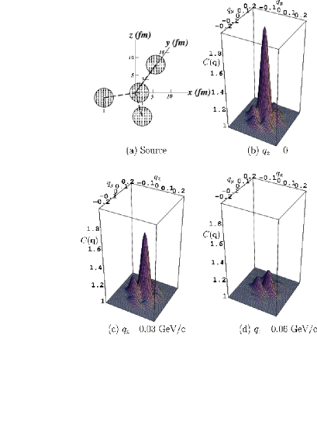
Figure 1: (a) A sample spatial configuration of four droplets. We use dashed lines to join the droplet centers and the origin to show the locations of the droplets. We use vertical dashed lines to indicate the projection of the droplet centers onto the $x-y$ plane. (b) Two-boson correlation function $C(q_{x},q_{y},q_{z})$ for $q_{z}=0,$ (c) for $q_{z}=0.030$ GeV/c, and (d) $q_{z}=0.06$ GeV/c. The quantities $q_{x}$ and $q_{y}$ are in units of GeV/c.

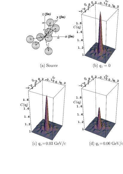
Figure 2: (a) A sample configuration of eight droplets. We use dashed lines to join the droplet centers and the origin to show the locations of the droplets. We use vertical dashed lines to indicate the projection of the droplet centers onto the $x-y$ plane. (b) Two-boson correlation function $C(q_{x},q_{y},q_{z})$ as a function of $q_{x}$ and $q_{y}$ at $q_{z}=0,$ (c) $q_{z}=0.03$ GeV/c, and (d) $q_{z}=0.06$ GeV/c. The quantities $q_{x}$ and $q_{y}$ are in units of GeV/c.

In our numerical example, we randomly select the localized droplet centers according to the distribution of Eq. (39) with $\sigma_{R}=4$ fm and take $\sigma_{d}=1.5$ fm for the standard deviation of the droplet. To avoid overlapping droplets, we require the droplets be separated by a distance greater than the sum of their root-mean-square radii, $2\sqrt{3}\sigma_{d}$. After the positions of the centers of the droplets are selected, we evaluate the correlation function $C({\bf q})$ with Eq. (35). A sample result for $N=4$ droplets is shown in Fig. 1, and another sample result for $N=8$ droplets is shown in Fig. 2. Figs. (1a) and (2a) show the spatial configurations of the droplets; Figs. (1b) and (2b) give the correlation functions $C({\bf q})$ as a function of $q_{x}$ and $q_{y}$ for $q_{z}=0$, Figs. (1c) and (2c) for $q_{z}=0.03$ GeV/c, and Figs. (1d) and (2d) for $q_{z}=0.06$ GeV/c. The momenta $q_{x}$ and $q_{z}$ in Figs. 1 and 2 are in units of GeV/c.

One observes from Figs. 1 and 2 that there are prominent fluctuations of the correlation function for a density distribution of localized droplets. The inversion symmetry $C(q_{x},q_{y},q_{z})=C(-q_{x},-q_{y},-qz)$ is present for $q_{z}=0$ (Figs. (1b) and (2b)). In addition to the maximum of $C(|{\bf q}|)$ at ${\bf q=0}$, there are maxima and minima at various locations of ${\bf q}$. The number of maxima for 8 droplets is greater than the number of maxima for 4 droplets.

The correlation functions for other configurations of 4 and 8 localized droplets exhibit similarly large fluctuations. On the average, the smaller the number of droplets, the greater will be the fluctuation. The magnitude of the fluctuation decreases as the number of droplets increases, as can be easily deduced from Eq. (35). The presence of this type of maxima and minima of a single-event correlation function at many relative momenta is a signature for a granular structure and a first-order QCD phase transition.

Because of the large fluctuations in a first-order phase transition, one expects that the locations of the centers of the droplets will be quite different from event to event. The large differences in the locations of the droplet centers in different events lead to large differences in the locations of the maxima and minima and large differences in the shapes of correlation functions (except for the maximum at ${\bf q}$=0).

It is interesting to examine the correlation function when we average over many events. The correlation function $C({\bf q})$ depends on the coordinates of the droplet centers, and the centers have a distribution $P({\bf R}_{j})$ in different events. The average of the correlation function over the different events, $\langle C({\bf q})\rangle$, is defined as

$$\langle C({\bf q})\rangle=\int\prod_{j=1}^{N}d{\bf R}_{j}P({\bf R_{j}})C({\bf q})\Biggr{/}\int\prod_{j=1}^{N}d{\bf R}_{j}P({\bf R_{j}}).$$ (40)

From Eq. (34) and the Gaussian distribution of the droplet centers (39), we obtain

$$\langle C({\bf q})\rangle=1+\frac{e^{-\sigma_{d}^{2}{\bf q}^{2}}}{N}+\frac{e^{-\sigma_{d}^{2}{\bf q}^{2}}}{N^{2}}\sum_{j=1}^{N}\sum_{k=1,k\neq j}^{N}\int\frac{d{\bf R}_{j}d{\bf R}_{k}}{(\sqrt{2\pi}\sigma_{R})^{6}}\exp\left\{-\frac{{\bf R}_{j}^{2}+{\bf R}_{k}^{2}}{2\sigma_{R}^{2}}+i{\bf q}\cdot({\bf R}_{j}-{\bf R}_{k})\right\},$$ (41)

and we get

$$\langle C({\bf q})\rangle=1+\frac{1}{N}e^{-\sigma_{d}^{2}{\bf q}^{2}}+\frac{N-1}{N}e^{-(\sigma_{d}^{2}+\sigma_{R}^{2}){\bf q}^{2}},$$ (42)

which is identical to the results of Pratt $et~{}al.$ for a pair of bosons from a distributed source Pra92 . Thus, the results of Pratt $et~{}al.$ Pra92 for a distributed source is the same as the results of averaging the correlation function over many different events. The average correlation function is now a relatively smooth function of $|{\bf q}|$, with only minor fluctuations even for only two and four droplets. The prominent fluctuations that are inherent in single-event correlation functions involving the term $\cos{\bf q}\cdot({\bf R}_{j}-{\bf R}_{k})$ in Eq. (35) are not present. The large fluctuations are now greatly suppressed by the averaging procedure.

In order to bring out the salient features of the correlation function, we have assumed in Eq. (31) that the source emission times $\{T_{j}\}$ for all droplets are the same. This is a reasonable assumption when the phase transition occurs over a short duration of time. The source function in Eq. (28) then factorizes in spatial and temporal coordinates. The correlation function $[C(q)-1]$ in Eq. (33) also factorizes in $q_{0}$ and ${\bf q}$, with $C({\bf q})$ given by Eq. (35).

On the other hand, if the phase transition occurs over a long duration, then the emission times $\{T_{j}\}$ can be different for different droplets. The source function Eq. (28) cannot be factorized as a product of spatial and temporal functions. Consequently, the correlation function $[C(q)-1]$ cannot be factorized and is given by the general result of Eq. (31). The correlation function $C(q)$ has maxima at $q=0$ and $q_{\rm max}\cdot{(X_{j}-X_{k})}\sim 2n\pi$, with $n=1,2,3,...$. It has minima at $q_{\rm min}\cdot{(X_{j}-X_{k})}\sim(2n-1)\pi$. The maxima and minima of the correlation function occur at relative momenta $q_{0}$ related to the relative emission time coordinates, $T_{j}-T_{k}$. The signature for the granular structure remains distinct, if one can make accurate measurements of the correlation function for different cuts in the relative momenta $q_{0}$.

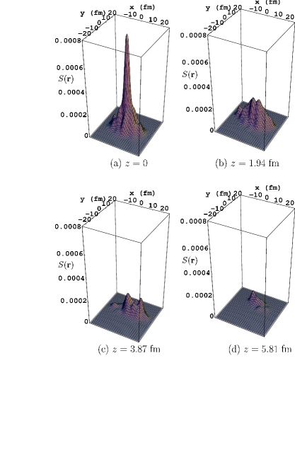
Figure 4: (a) The function $S(x,y,z)$ for 8 droplets in units of fm^-3 for the droplet distributions of Fig. 2. Fig. (4a) is for $S({\bf r})$ at $z=0$, (4b) for $S({\bf r})$ at $z=1.94$ fm, (4c) for $S({\bf r})$ at $z=3.87$ fm, and (4d) for $S({\bf r})$ at $z=5.81$ fm.

There are additional complications when one considers the internal hydrodynamical motion and the collective motion of the droplets relative to the center of mass. The hydrodynamics of a QGP droplet shows that the freeze-out radial coordinate in a QGP droplet is nearly independent of time in a first-order phase transition, when the initial energy density of the droplet is only slightly greater than $\epsilon_{c}$, the QGP energy density at the critical temperature $T_{c}$ (see Fig. 4(b) of Ref. [32]). As a droplet is presumably formed at temperatures near the critical temperature with an energy densities close to $\epsilon_{c}$, the assumption of the factorization of each droplet source as a product of spatial and temporal functions is reasonable for the case of a quark-gluon plasma with an initial temperature slightly above $T_{c}$.

For the case of a quark-gluon plasma with a high initial temperature much above $T_{c}$, the quark-gluon plasma will expand and cool. It will make a phase transition when it cools down to the critical temperature with the subsequent formation of granular droplets, if the phase transition is first-order in nature. At the moment of phase transition at $T_{c}$, the newly-formed droplets will acquire an expansion velocity moving away from the center of mass of the system. The factorization of the source function as a product of spatial and temporal functions is not possible, and the magnitude of the fluctuations of the correlation function may decrease. We shall investigate these effects on the correlation function in our future work.

V How to infer the density distribution from $C(q)$

The correlation function $C(q)$ is related to the Fourier transform of the density, $\tilde{\rho}(q)$. Information on $\rho(x)$ is encoded in $C(q)$. If the correlation function $C(q)$ has been measured experimentally as a function of its relative momentum coordinate $q$, then a proper Fourier transform of the correlation function will provide pertinent information on the density distribution $\rho(x)$.

We can obtain direct information on the density distribution $\rho(x)$ by decoding $C(q)$ in the following way. From the correlation function $C(q)$, one calculates $[C(q)-1]$, and one constructs the Fourier transform of $[C(q)-1]$,

$$S(x)=\int\frac{dq}{(2\pi)^{4}}e^{-iq\cdot x}[C(q)-1].$$ (43)

In the discussion of the Fourier transform (or the inversion) of the correlation function, the combination of the two terms in $[C(q)-1]$ always comes together. For simplicity, we shall often use the term ‘the Fourier transform (or the inversion) of the correlation function’ to mean ‘the Fourier transform (or the inversion) of $[C(q)-1]$’.

The function $S(x)$ is the two-particle ‘source function’ in the Koonin-Pratt formalismKon78 ; Pra90 and the imaging method of Brown, Danielewicz and their collaborators Bro97 ; Bro99 ; Bro04 ; Bro04a , for the special case for bosons without final-state interactions. Much progress has been made in obtaining a representation of this two-particle source function $S(x)$ in terms of spherical harmonics Bro97 ; Bro99 ; Bro04 ; Bro04a . For an irregular density distribution and correlation function as one encounters in granular droplets, an expansion of $S(x)$ in terms of spherical harmonics will not be adequate. The irregularity of the shape of the correlation function as shown in Figs. 1 and 2 calls for a more general method. The best method for inverting a general correlation function without symmetry is to use Cartesian coordinates in a three-dimensional Fourier transform. We have developed successfully a general three-dimensional Fast Fourier Transform method to invert highly irregular three-dimensional correlation functions. As described in details in Appendix A, our three-dimensional FFT method consists of performing a sequence of one-dimensional cosine and sine transforms in the three coordinate directions. In each of the cosine or sine transforms, we re-arrange the integral so that the limits of the integration go from zero to infinity and the integrand possesses the proper symmetric or antisymmetric reflectional symmetry, for cosine or sine transform respectively. We test our numerical three-dimensional FFT method by applying it to invert a correlation function of granular droplets for which results for the Fourier inversion can be easily obtained analytically.

In our analysis, we focus our attention on the source density function $\rho(x)$ itself as it directly gives the space-time configuration of the source. From the relation between $C(q)$ and $\rho(x)$ as given by Eq. (4), we get the integral equation for the source density function $\rho(x)$,

$${S}(x)=\int dx^{\prime}~{}\rho(x^{\prime})~{}\rho(x^{\prime}+x).$$ (44)

We can prove that $S(x)$ possesses inversion symmetry

$${S}(x)=S(-x).$$ (45)

The function ${S}(x)$ is not the source density but is the folding of the source density with itself. To focus our attention on the source density $\rho(x)$ and to emphasize the property of $S(x)$ as the folding of $\rho(x)$ with $\rho(x)$, we can call the function $S(x)$ alternatively as ‘the folding function’ of $\rho(x)$ in the discussion of the source density $\rho(x)$, in addition to the name of ‘the source function’ in the Koonin-Pratt formalism Kon78 ; Pra90 and imaging methods Bro97 ; Bro99 ; Bro04 ; Bro04a . The folding function $S(x)$ is real and positive definite. The same folding function $S(x)$ is obtained whether one uses $e^{-iq\cdot x}$ or its complex conjugate $e^{iq\cdot x}$ in the Fourier transform expression in Eq. (43).

We can illustrate the application of the folding function $S(x)$ with the example of the chaotic source of $N$ Gaussian density droplets, Eq. (28), studied in the last section. For such a granular source density $\rho(x)$, the folding function $S(x)$ can be obtained analytically. By carrying out the folding integration using Eq. (44), the folding function $S(x)$ can be easily found to be

$${S}(x)=A^{2}\sum_{j,\,k=1}^{N}\frac{1}{(\sqrt{2\pi}\sigma_{jk})^{3}\sqrt{2\pi}\tau_{jk}}\exp\left\{-\frac{[{\bf r}-({\bf R}_{j}-{\bf R}_{k})]^{2}}{2\sigma_{jk}^{2}}-\frac{[t-(T_{j}-T_{k})]^{2}}{4\tau_{jk}^{2}}\right\}.$$ (46)

where $\sigma_{jk}^{2}=\sigma_{j}^{2}+\sigma_{k}^{2}$ and $\tau_{jk}^{2}=\tau_{j}^{2}+\tau_{k}^{2}$. The function $S(x)$ has maxima at ${\bf r}=({\bf R}_{j}-{\bf R}_{k})$ and $t=(\tau_{j}-\tau_{k})$, in addition to the maxima at $x=0$. For simplicity, we again assume that $\sigma_{j}=\sigma_{d}$ and $\tau_{j}=\tau_{d}$ for all $j$. The function $S(x)$ for the granular droplets is simplified to be

$${S}(x)=\frac{1}{N^{2}(\sqrt{4\pi}\sigma_{d})^{3}\sqrt{4\pi}\tau_{d}}\sum_{j,\,k=1}^{N}\exp\left\{-\frac{[{\bf r}-({\bf R}_{j}-{\bf R}_{k})]^{2}}{4\sigma_{d}^{2}}-\frac{[t-(T_{j}-T_{k})]^{2}}{4\tau_{d}^{2}}\right\}.$$ (47)

Thus, if the folding function near the maxima does not overlap, the folding function $S(x)$ has maxima at locations governed by the relative coordinates of the droplet centers.

We can consider the case when the droplets are all produced at the same time, as for example when the droplets are produced at the moment of phase transition. Then the time $T_{j}$ can be taken to be the same for all $j$. The four-dimensional folding function $S(x)$ factorizes into a three-dimensional part $S({\bf r})$ and a normalized Gaussian distribution in time,

$$S(x)=S({\bf r})\frac{e^{-t^{2}/4\tau_{d}^{2}}}{\sqrt{4\pi}\tau_{d}},$$ (48)

where we use the same symbol $S$ for the three- and four-dimensional folding function. The ambiguity of the meaning of $S$ can be easily resolved by context and by its argument. The three-dimensional folding function $S({\bf r})$ is

$$S({\bf r})=\frac{1}{N^{2}(\sqrt{4\pi}\sigma_{d})^{3}}\sum_{j,\,k=1}^{N}\exp\left\{-\frac{[{\bf r}-({\bf R}_{j}-{\bf R}_{k})]^{2}}{4\sigma_{d}^{2}}\right\}.$$ (49)

If the folding function near the maxima does not overlap, the maxima of the three-dimensional function $S({\bf r})$ are located at

$${\bf r}={\bf R}_{j}-{\bf R}_{k},~{}~{}~{}~{}~{}~{}~{}~{}~{}~{}~{}~{}j,k=1,2,...N.$$ (50)

In Eq. (49) for $S({\bf r})$, there are $N$ terms with $j=k$, and these terms contribute additively to the maxima at ${\bf r}=0$. The height at the maxima at ${\bf r}=0$ is therefore $N$ times higher than the maximum with $j\neq k$ located at the the relative coordinates ${\bf R}_{j}-{\bf R}_{k}$. The occurrence of this type of maxima in $S({\bf r})$, in addition to the maxima at ${\bf r}=0$, provides another signature for a granular structure of the source and a first-order phase transition of the quark-gluon plasma.

The density distribution we have considered, with both $\tau_{j}$ and $T_{j}$ separately the same for all $j$, is a special case of those density distributions whose spatial and time distributions can be factorized: $\rho(x)=f(t)\rho({\bf r})$, where we use the same symbol $\rho$ for the three-dimensional and the four-dimensional density function. For these factorizable density distributions,

$$C(q)-1=|\tilde{f}(q_{0})|^{2}[C({\bf q})-1],$$ (51)

and

$$C({\bf q})-1=|\tilde{\rho}({\bf q})|^{2},$$ (52)

where $\tilde{f}(q_{0})$ and $\tilde{\rho}({\bf q})$ are the Fourier transforms of $f(t)$ and $\rho({\bf r})$, respectively. Consequently, the function $S(x)$ also factorizes and is given by

$$S(x)=S({\bf r})\int\frac{dq_{0}}{2\pi}e^{-iq_{0}t}|\tilde{f}(q_{0})|^{2},$$ (53)

where the three-dimensional function $S({\bf r})$ is equal to

$$S({\bf r})=\int\frac{d{\bf q}}{(2\pi)^{3}}e^{i{\bf q}\cdot{\bf r}}[C({\bf q})-1].$$ (54)

It is of interest to demonstrate the feasibility and the accuracy of the FFT method by using it to invert a correlation function and comparing the inversion result with the analytical result. We use the numerical correlation function $C({\bf q})$ obtained in our previous examples in Section IV (results as shown in Fig. 1 and 2) as input, and carry out the three-dimensional FFT of the correlation function $[C({\bf q})-1]$ to obtain $S({\bf r})$, as given in Eq. (54). The input correlation functions correspond to those of the localized configurations of Figs. (1a) and (2a).

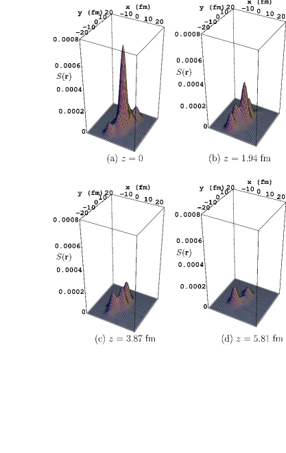
Figure 3: (a) The folding function $S(x,y,z)$ for 4 droplets in units of fm^-3 for the droplet configuration of Fig. 1. Fig. (3a) is for $S({\bf r})$ at $z=0$, (3b) for $S({\bf r})$ at $z=1.94$ fm, (3c) for $S({\bf r})$ at $z=3.87$ fm, and (3d) for $S({\bf r})$ at $z=5.81$ fm.

We show in Figs. 3 and 4 the results of the function $S({\bf r})$ at $z=0,1.94,3.87,$ and 5.81 fm obtained by inverting the correlation functions using the FFT method. Fig. 3 gives $S({\bf r})$ for the example of 4 droplets of Fig. 1. Fig. 4 gives $S({\bf r})$ for the example of 8 droplets of Fig. 2. One observes that besides the maxima at ${\bf r}=0$, the folding function $S({\bf r})$ has many maxima at ${\bf r}={\bf R}_{j}-{\bf R}_{k}$ where $j,k=1,...N$ and $j\neq k$. A granular structure shows up as having many maxima in the Fourier transform of $[C({\bf q})-1]$, in addition to the maxima at ${\bf r}=0$. For the case with 4 droplets in Fig. 3, the maxima of $S({\bf r})$ are quite distinctly exhibited. For the case with 8 droplets, the number of maxima increases and many maxima merge. However, some individual maxima remain distinctly separated as in Figs. (4b) and (4c).

To study the shape of the function $S(x)$ in more detail, we consider a cut at the plot of Fig. 3 at $x=0$, and plot $S(x=0,y,z)$ as a function of $y$ for different values of $z$ in Fig. 5. The results in Fig. (5a) and (5b) have been obtained by using the Fast Fourier Transform method for the example of 4 droplets of Fig. 1. Fig. (5a) gives $S(0,y,z)$ in linear scale and (5b) in logarithmic scale. One sees clearly oscillations of the folding function $S(x)$ due to the maxima at various ${\bf R}_{j}-{\bf R}_{k}$ locations. A signature for granular droplets is the presence of this type of maxima of the Fourier transform of $[C({\bf q})-1]$ at various spatial locations.

We can assess the accuracy of inverting a numerical correlation function with our Fast Fourier Transform method by comparing its results with the exact analytical result as given by Eq. (49). The exact analytical results of $S({\bf r})$ versus $y$ for $x=0$ and different $z$ values are shown in linear scale in Fig. (5c) and in logarithmic scale in Fig. (5d). The results from the FFT method match the exact analytical results with a very high degree of accuracy, including the detailed shapes of the oscillations and the values of $S({\bf r})$ down to the low density region of $y\sim\pm 30$ fm where $S({\bf r})$ is down by 6 orders of magnitude from its maximum value at ${\bf r}=0$. We have successfully developed an accurate three-dimensional FFT method to invert a correlation function $[C({\bf r})-1]$ to obtain its three-dimensional Fourier transform $S({\bf r})$.

The folding function $S({\bf r})$ will be distorted as noises are introduces into the correlation function. The degree of distortion will depend on the magnitude of the noise and it would be of interest to see how well the folding function can be determined with noises associated with experimental measurements. The high degree of accuracy in the FFT method makes it encouraging to apply it to determine the folding function $S({\bf r})$ for the investigation of the source density distribution $\rho({\bf r})$.

In order to facilitate the application of the three-dimensional Fourier transform using the experimental single-event correlation function $[C({\bf q})-1]$ (or perhaps functions that fit the experimental correlation function), we give the detailed steps of how the three-dimensional Fourier transform can be evaluated in Appendix A. The computer program to carry out the three-dimensional Fast Fourier Transform to obtain $S({\bf r})$ from $[C({\bf q})-1]$ can also be obtained from the authors upon request. Brown $et~{}al.$ have pointed out that in practical applications, when the experimental errors are large, it is important to include the error uncertainties into the equation for the inversion of the correlation function Bro97 ; Bro99 ; Bro04 ; Bro04a . Brown Bro99 also pointed out that when one applies the FFT transform to experimental correlation functions, one should take care to treat the experimental error in the measurement by filtering out the noise, and the best method is one in which the errors of the measurement are included in the inversion method.

It is worth emphasizing that Eq. (44), which connects the Fourier transform of the correlation function $[C(q)-1]$ to the density function $\rho(x)$, is a general result. It can be used to obtain other density distributions, in addition to the granular density distribution discussed here. Thus, if the correlation function $C(q)$ is experimentally determined, one can first evaluate the Fourier transform of $[C(q)-1]$, which gives the function $S(x)$. The integral equation Eq. (44) can then be used to determine the density distribution $\rho(x)$ by algebraic methods. In the three-dimensional case, one can discretize the integral equation Eq. (44) as

$${S}(i,j,k)=\Delta x\Delta y\Delta z\sum_{i^{\prime},j^{\prime},k^{\prime}=1}^{N}\rho(i+i^{\prime},j+j^{\prime},k+k^{\prime})\rho(i^{\prime},j^{\prime},k^{\prime}),$$ (55)

where $x=i\Delta x$, $y=j\Delta y$, and $z=k\Delta z$. We consider only the region of $S(x)$ and $\rho(x)$ inside the box of $i,j,k=1$ to $N$ and assume that they are zero outside the box.

With the determination of $S({\bf r})$ from a given experimental correlation function by the FFT method, one can in principle solved the above equation to obtain the source density distribution $\rho({\bf r})$. One can for example solve the above equation by iteration. In the first iterative step, one uses a initial guessed density distribution $\rho^{(0)}({\bf r})$ as one of the two density functions in Eq. (55). The equation is then a linear equation of $\rho({\bf r})$ and can be easily solved. The steps to obtain the solution is described in Appendix B. The solution $\rho({\bf r})$ can then be substituted into Eq. (55) to replace one of the two $\rho$ functions and to continue the iteration. Clearly, the iterative solution $\rho({\bf r})$ will be the solution of Eq. (44) or (55) if the iteration converges. The successes of the iterative solution will probably depend on a good initial guessed solution. It will be of great interest to test how this iterative procedure may be used to find a density distribution $\rho({\bf r})$ for a given experimental correlation function $C({\bf q})$. It is necessary to investigate how one can guarantee positive-definite solutions of $\rho({\bf r})$ in such procedure. Future development to search for methods to solve the integral equation Eq. (44) [or (55)] for $\rho(x)$ from a given $S(x)$ will be of great interest.

VI Conclusions and Discussions

Recent experiments at RHIC provide ample evidence for a dense matter produced in high-energy heavy ion collisions. Is the produced dense matter the quark-gluon plasma? An unambiguous identification of the produced matter as a quark-gluon plasma requires the observation of the phase transition from the new form of matter to known hadronic matter.

The signature for a phase transition depends on the order of the phase transition. Witten and many workers noted previously that a granular structure of droplets occurs in a first-order QCD phase transition, and the observation of the granular structure can be used as a signature for a first-order QCD phase transition Wit84 -Ran04a . HBT interferometry is the best experimental tool to examine the space-time density distribution of the produced matter. It can therefore be utilized to study the granular structure that occurs in a first-order phase transition of the plasma.

In the dynamics following a first-order QCD phase transition, the evolved matter will react chemically and thermally. It is not known how much the granular density pattern of the phase transition will remain to make it detectable by HBT interferometry. It has been argued in conventional theory that HBT interferometry measures the density distribution of the hadron matter at thermal freeze-out, as the re-scattering of bosons is assumed to lead to a chaotic configuration. This traditional assumption is subject to question as it was, however, pointed out recently that the propagation of bosons in the re-scattering process should be investigated in a quantum description Won03 ; Won04 ; Zha04a ; Kap04 . Upon using the Glauber theory to describe the scattering process, it was found that HBT interferometry measures the initial chaotic density distribution modified by absorption and collective flow Won03 ; Won04 . The HBT interferometry may be sensitive to the density distribution that occurs earlier than the thermal freeze-out configuration. If the initial density fluctuation is large, a substantial density fluctuation of the granular pattern may remain to make it detectable by HBT interferometry.

Whatever the theoretical predictions on the possible evolution of the produced matter may be, it is ultimately an experimental question whether a granular density distribution that occurs at the moment of the phase transition may subsequently render itself detectable by the available experimental tool of HBT interferometry.

We propose new ways to detect a granular density structure using the single-event HBT interferometry. If it can be carried out with sufficient accuracy, the single-event HBT interferometry can reveal the density distribution in each single event. It can also reveal large fluctuations in the density distribution from event to event, as is expected in a first-order phase transition.

We carry out our analysis with many examples of granular sources. We found that a granular structure is characterized by large fluctuations of the single-event correlation function. A single-event correlation function has maxima and minima at relative momenta that depend on the relative coordinates of the droplet centers. The presence of this type of maxima and minima of the single-event correlation function can be used as the signature for a granular structure and the first-order QCD phase transition of the quark-gluon plasma.

If an experimental single-event correlation function is complete and accurate enough, another very simple method to search for a granular structure is to take the Fourier transform of the correlation function. The Fourier transform of the correlation function leads to the folding of the source density with itself. This Fourier transform possesses maxima at spatial coordinates governed by the relative coordinates of the droplet centers. The occurrence of this type of maxima in the Fourier transform, in addition to the maxima at ${\bf r}=0$, is another signature for granular droplets and a first-order quark-gluon plasma phase transition.

In the present analysis, we have focused our attention on the single-event HBT interferometry to emphasize the maximum fluctuations in the correlation function of a granular structure. It will be of great interest to study a few-event HBT analysis both theoretically and experimentally. The few-event HBT analysis will be necessary for practical reasons, if the number of boson pairs in a single event is not large enough to provide sufficient statistics. The few-event HBT analysis will also be needed to understand the degrees of fluctuation from event to event. One wishes to find out whether the fluctuations in few-event HBT correlation measurements contain a single-event component that is beyond statistical fluctuations. The rate of the change of the degrees of fluctuation as the number of events increases will provide information on the underlying fluctuations in the single-event and event-to-event HBT interferometry. The successful development of the single-event or few-event HBT interferometry in high-energy heavy-ion collisions will open up a vast vista for future exploration.

In the present investigation, we have considered idealized situations in order to bring out the most important features of the signature for a granular structure. It will be of great interest to examine in future work how the signature discussed here may be affected when some of our simplifying assumptions are modified. The determining factor for the occurrence of maxima and minima in the correlation function $C({\bf q})$ is the interference of two histories for two bosons to propagate from two source points in different droplets to the detecting points. This interference involves a phase difference which depends on the radius vector joining the two droplets. If this underlying factor of interference leading to large fluctuations of the correlation function remains important even after modifying our simplifying assumptions, then many of the gross features obtained here will not be greatly modified.

The fluctuations arising from a granular structure described in the present idealized theoretical investigation will be blurred by experimental statistical fluctuations due to the limited number of experimental counts. Whether or not the relevant signal can be recovered in the presence of experimental statistical fluctuations remains to be tested. Clearly, the smaller the number of droplets, the greater is the signal and the greater will be the probability of its observation in the presence of statistical fluctuations. It will be of great interest to carry out a theoretical simulation to see what are the minimum droplet size and the largest droplet number a given experimental arrangement may be able to detect.

Much work remains to be done both experimentally and theoretically to investigate this interesting topic on the signature of the phase transition of the quark-gluon plasma. It will be of interest to study theoretically effects of the collective expansion of the sources and the droplets, effects of fluctuations of the size of the droplets, effects of absorption of the bosons on its way to the detector, effects of the momentum dependences of the density distributions, and other interesting questions in connection with the signature of the granular structure.

Appendix A Evaluation of the three-dimensional Fourier transform of the correlation function $[C({\bf q})-1)]$

From Eq. (54), we have

$$S({\bf r}) = \int\frac{d{\bf q}}{(2\pi)^{3}}e^{-i{\bf q}\cdot{\bf r}}[C({\bf q})-1]$$ (56)

$$= \int\frac{d{\bf q}}{(2\pi)^{3}}\{\cos({\bf q}\cdot{\bf r})+i\sin({\bf q}\cdot{\bf r})\}[C({\bf q})-1].$$

The imaginary part in the above integration vanishes as $C(-{\bf q})=C({\bf q})$. It is only necessary to evaluate the real part of the Fourier transform. The folding function $S({\bf r})$ is therefore

$$S({\bf r})=\int\frac{d{\bf q}}{(2\pi)^{3}} \cos(q_{x}x+q_{y}y+q_{z}z)~{}R({\bf q}),$$ (57)

where $R({\bf q})=C({\bf q})-1$. Expanding the cosine function, we obtain

$$S({\bf r})=\int\frac{d{\bf q}}{(2\pi)^{3}} [\cos q_{x}x\cos q_{y}y\cos q_{z}z-\cos q_{x}x\sin q_{y}y\sin q_{z}z$$ (58)

$$~{}~{}-\sin q_{x}x\cos q_{y}y\sin q_{z}z-\sin q_{x}x\sin q_{y}y\cos q_{z}z]~{}R({\bf q}).$$

In the standard numerical subroutines such as those in the Fast Fourier Transform package of DFFTPACK FFT , the cosine transform of an even function of $G(q)$ is usually approximated by

$$\tilde{G}(x)=\int_{0}^{\infty}dq~{}\cos(qr)G(q)=\Delta q\sum_{j=1}^{N}\cos\{(j-1)(k-1)\pi/N\}G(q),$$ (59)

where $x=(k-1)\Delta x$, $q=(j-1)\Delta q$, and $(\Delta x)(\Delta q)=\pi/N$ . The right-hand side quantities are then calculated by the one-dimensional cosine Fast Fourier Transform subroutine of the package. Similarly, the sine transform of an odd function is usually approximated by

$$\tilde{G}(x)=\int_{0}^{\infty}dq~{}\sin(qr)G(q)=\Delta q\sum_{j=1}^{N}\sin\{jk\pi/(N+1)\}G(q),$$ (60)

with $x=k\Delta x$ and $q=j\Delta q$ and $\Delta x\Delta q=\pi/(N+1)$.

The Fourier integral of the sine and cosine function in Eq. (58) can be cast into the standard form of Eqs. (59) and (60) in the FFT package of DFFTPACK by noting that

$$\int_{-\infty}^{\infty}dq_{x}~{}\cos q_{x}x~{}g(q_{x},q_{y},q_{z})=\int_{0}^{\infty}dq_{x}~{}\cos q_{x}x\,[g(q_{x},q_{y},q_{z})+g(-q_{x},q_{y},q_{z})],$$ (61)

and similarly

$$\int_{-\infty}^{\infty}dq_{x}~{}\sin q_{x}x~{}g(q_{x},q_{y},q_{z})=\int_{0}^{\infty}dq_{x}~{}\sin q_{x}x\,[g(q_{x},q_{y},q_{z})-g(-q_{x},q_{y},q_{z})].$$ (62)

Using the above results, the four terms inside the square bracket in Eq. (58) lead to four contributions to $S({\bf r})$,

$$S({\bf r})=[A_{1}({\bf r})-A_{2}({\bf r})-A_{3}({\bf r})-A_{4}({\bf r})]/(2\pi)^{3},$$ (63)

where

$$A_{1}(x,y,z)=\int_{0}^{\infty}dq_{z}~{}\cos{q_{z}z}[F_{1}(x,y,q_{z})+F_{1}(x,y,-q_{z})],$$ (64)

$$F_{1}(x,y,q_{z})=\int_{0}^{\infty}dq_{y}~{}\cos{q_{y}y}[E_{1}(x,q_{y},q_{z})+E_{1}(x,-q_{y},q_{z})],$$ (65)

and

$$E_{1}(x,q_{y},q_{z})=\int_{0}^{\infty}dq_{x}~{}\cos{q_{x}x}\left[R(q_{x},q_{y},q_{z})+R(-q_{x},q_{y},q_{z})\right].$$ (66)

The term $A_{2}$ that contributes to $S(x)$ can be obtained similarly as

$$A_{2}(x,y,z)=\int_{0}^{\infty}dq_{z}~{}\sin{q_{z}z}[F_{2}(x,y,q_{z})-F_{2}(x,y,-q_{z})],$$ (67)

$$F_{2}(x,y,q_{z})=\int_{0}^{\infty}dq_{y}~{}\sin{q_{y}y}[E_{2}(x,q_{y},q_{z})-E_{2}(x,-q_{y},q_{z})],$$ (68)

and

$$E_{2}(x,q_{y},q_{z})=\int_{0}^{\infty}dq_{x}~{}\cos{q_{x}x}\left[R(q_{x},q_{y},q_{z})+R(-q_{x},q_{y},q_{z})\right].$$ (69)

In a similar way, the term $A_{3}(x,y,z)$ is given by

$$A_{3}(x,y,z)=\int_{0}^{\infty}dq_{z}~{}\sin{q_{z}z}[F_{3}(x,y,q_{z})-F_{3}(x,y,-q_{z})],$$ (70)

$$F_{3}(x,y,q_{z})=\int_{0}^{\infty}dq_{y}~{}\cos{q_{y}y}[E_{3}(x,q_{y},q_{z})+E_{3}(x,-q_{y},q_{z})],$$ (71)

and

$$E_{3}(x,q_{y},q_{z})=\int_{0}^{\infty}dq_{x}~{}\sin({q_{x}x})\left[R(q_{x},q_{y},q_{z})-R(-q_{x},q_{y},q_{z})\right].$$ (72)

Finally, $A_{4}(x,y,z)$ is given by

$$A_{4}(x,y,z)=\int_{0}^{\infty}dq_{z}~{}\cos{q_{z}z}[F_{4}(x,y,q_{z})+F_{4}(x,y,-q_{z})],$$ (73)

$$F_{4}(x,y,q_{z})=\int_{0}^{\infty}dq_{y}~{}\sin{q_{y}y}[E_{4}(x,q_{y},q_{z})-E_{4}(x,-q_{y},q_{z})],$$ (74)

and

$$E_{4}(x,q_{y},q_{z})=\int_{0}^{\infty}dq_{x}~{}\sin{q_{x}x}\left[R(q_{x},q_{y},q_{z})-R(-q_{x},q_{y},q_{z})\right].$$ (75)

The right-hand sides of the above equations (64)-(75) are now in the form of the sine and cosine integrals of Eqs. (59) and (60), for which standard FFT subroutines can be applied. With the above relations, the folding function $S({\bf r})$ can be easily evaluated using subroutines in standard Fast Fourier Transform packages.

Incidentally, we have shown how we can obtain the 3-dimensional Fourier transform for a function that is symmetric with respect to the inversion of its coordinates, for which the imaginary part of the Fourier transform vanishes. For other general functions without such a symmetry, the imaginary Fourier component involving $\sin({\bf q}\cdot{\bf r})$ does not vanish. We can expand the function $\sin(q_{x}x+q_{y}y+q_{z}z)$ as in Eq. (58) and use techniques similar to those in Eqs. (63)-(75) to get the imaginary part of the Fourier transform.

Appendix B Solution of the discretized integral equation

We wish to obtain an iterative solution of the discretized integral equation (55) for $\rho({\bf r})$, with a given $S({\bf r})$. As the density function $\rho({\bf r})$ is zero outside the box of $\{i,j,k=1$ to $N\}$. the summation in Eq. (55) can be limited to density functions inside the box. Consequently, Eq. (55) contains fewer and fewer numbers of unknown variables of $\rho$ as the indices $i$, $j$, or $k$ of $S(i,j,k)$ increases. We can choose our starting point to be the linear equation containing only one variable. The equation can be easily solved. The variables in the subsequent set of linear equation can be solved in sequence. Similar procedures can be carried out in two and three dimensions. We shall give the detail procedures below for the one-dimensional case to indicate how the iterative solution can be obtained.

We seek an iterative solution of $\rho(i)$ satisfying

$$S(i)/\Delta x=\sum_{i^{\prime}=1}^{N}\rho(i+i^{\prime})\rho^{(0)}(i^{\prime}),$$ (76)

where $\rho^{(0)}(i^{\prime})$ is either a guessed solution or the solution of the previous iteration.

Because the density function is zero outside the region of $i<1$ and $i>N$, the set of equations of (76) are

$$S(N)=0,$$ (77)

$$S(N-1)/\Delta x=\rho(N)\rho^{(0)}(1),$$ (78)

$$S(N-2)/\Delta x=\rho(N-1)\rho^{(0)}(1)+\rho(N)\rho^{(0)}(2),$$ (79)

$$S(N-3)/\Delta x=\rho(N-2)\rho^{(0)}(1)+\rho(N-1)\rho^{(0)}(2)+\rho(N)\rho^{(0)}(3),....$$ (80)

$$S(1)/\Delta x=\rho(1)\rho^{(0)}(1)+\rho(2)\rho^{(0)}(2)+...+\rho(N)\rho^{(0)}(N).$$ (81)

Eq. (78) contains only a single unknown, $\rho(N)$, and can be solved in terms of the other known quantities. Knowing the value of $\rho(N)$, Eq. (79) can be solved for $\rho(N-1)$, and so on. In this way, the whole array of $\rho(i)$ can be determined. The above method can be easily generalized to calculate the iterative solution of the 3-dimensional density function $\rho({\bf r})$ from $S({\bf r})$. It will be necessary to normalize the density solution $\rho({\bf r})$ after each iterative step to ensure that the final solution has the proper normalization.

Appendix C Figures

Figure 5: The function $S(x=0,y,z)$ versus y for various values of $z$ for the 4 droplets examples of Figs. 1 and 3. The results from the FFT Method are given in linear scale in Fig. (5a) and in logarithmic scale in Fig. (5b). The results from the exact analytical solution of Eq. (49) are given in linear scale in Fig. (5c) and in logarithmic scale in Fig. (5d).

References

- (1) M. Gyulassy and L. McLerran, nucl-th/0405013.
- (2) See also New Discoveries at RHIC: the current case for the strongly interactive QGP, RIKEN Scientific Articles, Volume 9, BNL, May 14-15, 2004.
- (3) E. Witten, Phys. Rev. D30, 272 (1984).
- (4) D. Seibert, Phys. Rev. Lett. 63, 136 (1989).
- (5) T. Kajino, Phys. Rev. Lett. 66, 125 (1991).
- (6) S. Pratt, P. J. Siemens, and A. P. Vischer, Phys. Rev. Lett. 68, 1109 (1992).
- (7) L. P. Csernai and J. I. Kapusta, Phys. Rev. D46, 1379 (1992); L. P. Csernai and J. I. Kapusta, Phys. Rev. Lett. 69, 737 (1992).
- (8) R. Venugopalan and A. P. Vischer, Phys. Rev. E49, 5849 (1994).
- (9) W. N. Zhang, Y. M. Liu, L. Huo, Y. Z. Jiang, D. Keane, and S. Y. Fung, Phys. Rev. C51, 922 (1995).
- (10) S. Alamoudi , Phys. Rev. D60, 125003 (1999).
- (11) W. N. Zhang, G. X. Tang, X. J. Chen, L. Huo, Y. M. Liu, and Z. Zhang, Phys. Rev. C62, 044903 (2000).
- (12) L. P. Csernai, J. I. Kapusta, and E. Osnes, Phys. Rev. D67, 045003 (2003).
- (13) J. Randrup, Phys. Rev. Lett. 92, 122301 (2004).
- (14) W. N. Zhang, M. J. Efaaf, C. Y. Wong, Phys. Rev. C70, 024903 (2004).
- (15) J. Randrup, nucl-th/0406031.
- (16) For a general review of the Hanbury-Brown-Twiss intensity interferometry, see Chapter 17 of C. Y. Wong, Introduction to High-Energy Heavy-Ion Collisions, World Scientific Publishing Company, 1994.
- (17) R. Hanbury-Brown and R. Q. Twiss, Phil. Mag. 45, 633 (1954); R. Hanbury-Brown and R. Q. Twiss, Phil. Mag. Nature 177, 27 (1956); R. Hanbury-Brown and R. Q. Twiss, Phil. Mag. Nature 178, 1046, (1956).
- (18) R. J. Glauber, Phys. Rev. Lett. 10, 84 (1963); R. J. Glauber, Phys. Rev. 130, 2529 (1963); R. J. Glauber, Phys. Rev. 130, 2766 (1963).
- (19) S. E. Koonin, Phys. Lett. B70, 43 (1977); F. B. Yano and S. E. Koonin, Phys. Lett. B78, 556 (1978).
- (20) S. Y. Fung, W. Gorn, G. P. Kiernan, J. J. Lu, Y. T. Oh, and R. T. Poe, Phys. Rev. Lett. 41, 1592 (1978).
- (21) M. Gyulassy, S. K. Kauffman, and L. W. Wilson, Phys. Rev. C20, 2267 (1979).
- (22) S. Pratt, Phys. Rev. Lett. 53, 1219 (1984).
- (23) S. Pratt, Phys. Rev. D33, 72 (1986); S. Pratt, Phys. Rev. D33, 1314 (1986).
- (24) Y. Hama and S. S. Padula, Phys. Rev. D37, 3237 (1988).
- (25) G. F. Bertsch, Nucl. Phys. A498, 173c (1989).
- (26) Yu. M. Sinyukov, Nucl. Phys. A498, 151c (1989).
- (27) S. Pratt, T. Csörgö and T. Zimányi, Phys. Rev. C42, 2646 (1990).
- (28) D. Boal, C.-K. Gelbke, and B. K. Jennings, Rev. Mod. Phys. 62, 553 (1990).
- (29) W. Bauer, C. K. Gelke, and S. Pratt, Ann. Rev. Nucl. Part. Sci. 42, 77 (1992).
- (30) W. A. Zajc, in Particle Production in Highly Excited Matter, Edited by H. H. Gutbrod and J. Rafelski, Plenum Press, New York, 1993, page 435.
- (31) V. Cianciolo, Ph. D. Thesis, M.I.T., 1994.
- (32) D. H. Rischke and M. Gyulassy, Nucl. Phys. A608, 479 (1996).
- (33) D. A. Brown and P. Danielewicz, Phy. Lett. B398, 252 (1977); D. A. Brown and P. Danielewicz, Phy. Rev. C57, 2474 (1998); D. A. Brown and P. Danielewicz, Phy. Rev. C64, 014902 (2001).
- (34) U. Heinz and B. Jacak, Ann. Rev. Nucl. Part. Sci. 49, 529 (1992).
- (35) U. A. Wiedemann, U. Heinz, Phys. Rept. 319, 145-230 (1999).
- (36) D. Teaney and E. Shuryak, Phys. Rev. Lett. 83, 4951 (1999).
- (37) D. A. Brown, nucl-th/9904063.
- (38) R. M. Weiner, Phys. Rept. 327, 249 (2002).
- (39) C. Y. Wong, J. Phys. G29, 2151 (2003).
- (40) C. Y. Wong, J. Phys. G30, S1053 (2004).
- (41) W. N. Zhang, M. J. Efaaf, C. Y. Wong, and M. Khalilisr, Chin. Phys. Lett. 21, 1918 (2004), nucl-th/0404047.
- (42) J. Kapusta and Y. Li, J. Phys. G30, S1069 (2004).
- (43) D. A. Brown and P. Danielewicz, H. Heffner, and R. Stolz, Proc. 20th Winter Workshop on Nuclear Dynamics, nucl-th/0404067;
- (44) P. Danielewicz, D. A. Brown, H. Heffner, S. Pratt, and R. Stolz, nucl-th/0407022;
- (45) PHENIX Collaboration, K. Adcox et al., Phys. Rev. Lett. 88, 192302 (2002).
- (46) STAR Collaboration, C. Adler et al., Phys. Rev. Lett. 87, 082301 (2001).
- (47) S. Pratt, Nucl. Phys. A715, 389c (2003).
- (48) S. Soff, S. A. Bass, and A. Dumitru, Phys. Rev. Lett. 86, 3981 (2001).
- (49) S. Soff, S. A. Bass, D. H. Hardtke, and S. Y. Panitkin, J. Phys. G28, 1885 (2002).
- (50) S. Soff, S. A. Bass, D. H. Hardtke, and S. Y. Panitkin, Phys. Rev. Lett. 88, 072301 (2002).
- (51) U. Heinz and P. Kolb, Nucl. Phys. A702, 269 (2002).
- (52) D. Molnár and M. Gyulassy, in Proceedings of Budapest ’02 Workshop on Quark Hadron Dynamics, published in Heavy Ion Phys. 18, 69 (2003), nucl-th/0204062.
- (53) Zi-wei Lin, C. M. Ko, and S. Pal, Phys. Rev. Lett. 89, 152301 (2002).
- (54) D. Teaney, Nucl. Phys. A715, 817 (2003).
- (55) T. Csörgö and J. Zimányi, Acta Phys. Hung. New Series, Heavy-Ion Physics 17, 281 (2003), nucl-th/0206051.
- (56) D. Molnár and M. Gyulassy, Phys. Rev. Lett. 92, 052301 (2004).
- (57) J. Adams , the STAR Collaboration, nucl-ex/0311017.
- (58) G. Roland , (NA49 Collaboration), Nucl. Phys. A638, 91c (1998).
- (59) H. Applehäuser , (NA49 Collaboration), Phys. Lett. B459, 679 (1999).
- (60) S. V. Afasiev , (NA49 Collaboration), Phys. Rev. Lett. 86, 1965 (2001).
- (61) G. Baym and H. Heiselberg, Phys. Lett. B469, 7 (1999).
- (62) A. Bialas and V. Koch, Phys. Lett. B456, 1 (1999).
- (63) H. Heiselberg and A. D. Jackson, Phys. Rev. C63, 064904 (2001).
- (64) V. Koch, M. Bleicher, and S. Jeon, Nucl. Phys. A698, 261c (2002).
- (65) J. Schukraft, Nucl. Phys. A698, 287 (2002).
- (66) H. C. Pumphrey and P N Swarztrauber, DFFTPACK Package, available from the fftpack site in www.netlib.org.