Model Calculation of Effective Three-Body Forces

Abstract

We propose a scheme for extracting an effective three-body interaction originating from a two-nucleon interaction. This is based on the $\hat{Q}$-box method of Kuo and collaborators, where folded diagrams are obtained by differentiating a sum of non-folded diagrams with respect to the starting energy. To gain insight we have studied several examples using the Lipkin model where the perturbative approach can be compared with exact results. Numerically the three-body interactions can be significant and in a matrix example good accuracy was not obtained simultaneously for both eigenvalues with two-body interactions alone.

I Introduction

The role of effective three-body forces in shell-model and nuclear structure calculations of medium-heavy and heavy nuclei is still an unsettled question. The question has received scattered attention over the years, but there has been no decisive study yet yielding a unique answer, see for example Refs. herbert1 ; herbert2 ; herbert3 ; dehmo04 . Most of the studies seem to indicate that effective three-body forces play a rather modest role for nuclear spectra, although there is a possibility that binding energies may be more substantially affected. As pointed out by Zuker zuker1 , one is not able to obtain simultaneously a good reproduction of both the excitation spectra and the binding energy with effective interactions based on two-body nucleon-nucleon interactions only, unless one fits an effective interaction to reproduce selected data, see for example the recent work of Otsuka et al. in Refs. taka1 ; taka2 . To give an example, effective interactions derived from two-body nucleon-nucleon interactions which fit nucleon-nucleon scattering data, are not able to reproduce the well-known shell closure in ⁴⁸Ca nor the excitation spectra of ⁴⁷Ca and ⁴⁹Ca zuker1 ; alex ; oslo . For the chain of oxygen isotopes one may even reach the conclusion that ²⁸O is a bound nuclear system, unless the interaction is fitted to reproduce selected properties such as binding energies and spectra of known and stable nuclei in the $1s0d$ shell alex .

On the other hand, theoretical interactions which have not been fitted do rather well in reproducing nuclear properties other than binding energies and shell closures. Examples are nuclear spectra around $A\sim 100$ and $A\sim 132$ matej1 ; matej2 ; matej3 ; torgeir ; jo ; anne , which come out surprisingly well in view of the complexity of the many-body problem. It has therefore been speculated that some of the abovementioned deficiencies could be ascribed to the lack of three-body interactions, as seen in recent Monte Carlo and no-core shell-model calculations of light nuclei with $A\leq 16$ bob1 ; bob2 ; bob3 ; petr_erich2002 ; petr_erich2003 .

In light nuclei the role of three-body forces seems rather well established. To reproduce the binding energy of the triton, for example, it is necessary to include a three-nucleon interaction in addition to the two-nucleon interaction. The situation in medium-heavy and heavy nuclei is however unclear, although similar arguments, based on an analysis of $0p$, $1s0d$ and $1p0f$ nuclei by Zuker zuker1 lend support to the need for three-body interactions in heavier nuclei as well.

In contrast to the case for light nuclei, none of the present calculations of effective interactions for medium and heavy nuclei are sufficiently complete, however, to enable one to draw definite conclusions. For nuclei with $A>16$, one relies on shell-model analyses combined with appropriate effective interactions for a selected model space. Such interactions are typically based on perturbative many-body methods and because high-order calculations of the effective three-body contribution are prohibitively complicated, one is forced to limit oneself to low-order calculations. There are however classes of diagrams which can be summed to infinite order. One of these classes is the set of folded diagrams. The latter arise due to the removal of the dependence on the exact model-space energy in the Brillouin-Wigner perturbation expansion. Through the $\hat{Q}$-box formulation and its derivatives oslo ; ko , this set of diagrams can easily be summed up. With few exceptions herbert2 , three-body folded diagrams have not been included. There are indications, however, that folded three-body diagrams may be important, even if non-folded ones are small.

There is obviously a need to obtain a clearer picture of the role of effective three-body forces in heavier nuclei. Part of our motivation for studying the contribution of effective three-body forces comes from large-scale shell-model calculation of the entire range of Sn isotopes from A = 100 to A = 132, where the spectra are well reproduced whereas the binding energies are strongly overestimated. In fact, it was found that a small repulsive monopole contribution to the effective two-body interaction could cure this problem. The origin of such a term is unknown, but it is speculated that it might be simulating an effective three-body interaction. Indeed Talmi igal has shown that the binding energies of the entire range of Sn isotopes could be well fitted by an effective two-body plus an effective three-body interaction. In spite of the fact that both the Green’s function Monte Carlo and no-core shell-model approaches offer benchmark calculations of light nuclei with $A\leq 16$ bob1 ; bob2 ; bob3 ; petr_erich2002 ; petr_erich2003 , and that coupled cluster approaches can presently extend the region of ab initio calculations to $A\sim 40-56$ cc1 , features of heavier nuclei will most likely be studied within the framework of the shell model and appropriately defined effective interactions. Thus we need to have a controlled approach which allows us to discern contributions from various many-body terms, such as effective three-body forces. Effective three-body forces may originate from three-nucleon forces as well as from two-nucleon forces. In order to be able to draw definite conclusions, we believe that it is necessary to study one effect at a time. Thus, before introducing a three-nucleon interaction, we would study the contribution from effective three-body forces originating from the two-nucleon interaction. This is the topic of the present work.

The paper is organized as follows. In Sec. II we propose an algorithm for evaluating the effective three-body interaction in the convenient $\hat{Q}$-box formalism introduced by Kuo and collaborators ko ; oslo . We prepare ourselves for this procedure by briefly summarizing the method for obtaining the effective two-body interaction. Because the method can be rather involved in realistic cases, we apply it in Sec. III to a simple model, namely the Lipkin model LMG65 , for which exact results can easily be obtained, see for example Ref. vary04 . This is instructive both as regards the formalism and the numerical results. In the final Sec. IV we draw conclusions and point to the need for more realistic calculations.

II The Effective One-, Two- and Three-Body Interactions

The Hamiltonian acting in the complete Hilbert space (usually infinite) consists of an unperturbed one-body part, $H_{0}$, and a perturbation ${\cal V}$, namely $H=H_{0}+{\cal V}$. The goal is to obtain an effective interaction, $V$, such that $H=H_{0}+V$ acting in a chosen model or valence space yields a set of eigenvalues which are identical to (a subset of) those of the complete problem. To this end Kuo and collaborators introduced the $\hat{Q}$-box, see Refs. oslo ; ko , which, in principle, contains all non-folded diagrams which are attached to the valence particle lines. Unlinked pieces which refer to excitations of a closed-shell core are absent since the energy is calculated relative to the closed-shell ground state bran . The effective interaction also requires that folded diagrams be included to all orders and this can be formally written

$$V=\lim_{n\rightarrow\infty}V(n)\;,$$ (1)

where

$$V(n)=\hat{Q}(\omega)+\sum_{m=1}^{\infty}\frac{1}{m!}\frac{d^{m}\hat{Q}}{d\omega^{m}}\bigl{\{}V(n-1)\bigr{\}}^{m}\;,$$ (2)

with $V(0)\equiv\hat{Q}$ and matrix multiplication implied. Here $\omega$ is the unperturbed energy of the initial state. In order to perform calculations with $N$ particles in the model space it is necessary to separate the effective interaction $V$ into its one-, two- and three-body components (in principle up to $N$-body interactions are needed, but we shall not go beyond three-body). This brief sketch establishes our notation; a complete discussion is to be found in Refs. oslo ; ko ; bran ; usrev .

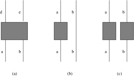
Figure 1: Two-body diagrams discussed in the text.

Consider first the case where our model space consists of a single particle, $N=1$; we assume that a given total angular momentum $j$ is represented only once. Then Eq. (1) can be solved for each state separately, yielding the complete folded series for the one-body effective interaction $V\equiv V^{(1)}$. The one-body effective Hamiltonian is thus $H_{0}+V^{(1)}$.

Now consider the case where we have two particles in the model space, $N=2$. The $\hat{Q}$-box again consists of all non-folded diagrams. It will include diagrams such that the interactions link the two valence lines together as indicated schematically in Fig. 1(a), diagrams where one line is non-interacting as in Fig. 1(b) and also diagrams where the interactions on each line are separate so that the diagram is valence unlinked as in Fig. 1(c). All of these components need to be included so as to generate the cross terms in the full folded effective interaction of Eqs. (1) and (2). Valence unlinked diagrams are removed by the folding process so that the effective interaction is completely linked bran . Now because of the one- plus two-body nature of the $\hat{Q}$-box, the result for $V$ from Eq. (1) will contain linked, folded two-body components which are schematically of the form of Fig. 1(a) plus linked, folded one-body components where one line is non-interacting, as in Fig. 1(b). The one-body piece $V^{(1)}$ is already determined, as indicated above, so the purely two-body interaction $V^{(2)}$ can be obtained from

$$\langle de|V|ab\rangle_{2}=\langle de|V^{(2)}|ab\rangle+\delta_{da}\delta_{eb}\Bigl{(}\!\langle a|V^{(1)}|a\rangle+\langle b|V^{(1)}|b\rangle\!\Bigr{)}.$$ (3)

The subscript on the left indicates the value of $N$ for which Eq. (1) is solved. We assume here that the initial and final states in Fig. 1(a) are in a standard order so that $e=a$ implies $d\neq b$. Here the two-body matrix elements are “antisymmetrized”, i.e $\langle de|V|ab\rangle$ implies $\langle de|V|ab-ba\rangle$. They are not coupled to a total angular momentum or isospin since our shell model calculations are carried out in the $m$-scheme.

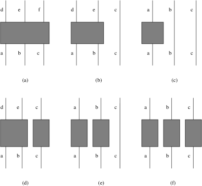
Figure 2: Three-body diagrams discussed in the text.

Turning to the more interesting three-body case ($N=3$), consider the $\hat{Q}$-box. It contains diagrams such that the interactions link the three valence lines together as indicated schematically in Fig. 2(a), diagrams where two of the lines are linked (Fig. 2(b)) or where only one line is interacting as in Fig. 2(c). The valence unlinked diagrams can involve a two-body and a one-body piece (Fig. 2(d)) or two or three one-body pieces (Figs. 2(e) and (f)). Notice that there are no valence unlinked diagrams if, as is often the case, one-body interactions are excluded. In general all of the components illustrated in Fig. 2 need to be included in generating the full folded, valence-linked effective interaction of Eqs. (1) and (2). The interaction has a three-body contribution where the three lines are linked together, schematically in the form of Fig. 2(a), two-body interactions acting on all possible pairs of lines (Fig. 2(b)) and one-body interactions acting each line separately (Fig. 2(c)). Using Eq. (3) we can disentangle the desired $V^{(3)}$ from

$$\langle def|V|abc\rangle_{3} = \langle def|V^{(3)}|abc\rangle+\delta_{fc}\langle de|V|ab\rangle_{2}-\delta_{fb}\langle de|V|ac\rangle_{2}+\delta_{fa}\langle de|V|bc\rangle_{2}+\delta_{eb}\langle df|V|ac\rangle_{2}$$ (4)

$$-\delta_{ec}\langle df|V|ab\rangle_{2}-\delta_{ea}\langle df|V|bc\rangle_{2}+\delta_{da}\langle ef|V|bc\rangle_{2}-\delta_{db}\langle ef|V|ac\rangle_{2}+\delta_{dc}\langle ef|V|ab\rangle_{2}$$

$$-\delta_{da}\delta_{eb}\delta_{fc}\Bigl{(}\langle a|V^{(1)}|a\rangle+\langle b|V^{(1)}|b\rangle+\langle c|V^{(1)}|c\rangle\Bigr{)}\;.$$

Again the subscript on the left indicates the value of $N$ for which Eq. (1) is solved. Of course for a given matrix element only a few of the delta functions will be nonzero. Since the inital and final states are in a chosen standard order the one-body term only contributes when $d=a$, $e=b$ and $f=c$. Here the uncoupled three-body matrix elements are “antisymmetrized”, i.e $\langle def|V|abc\rangle$ implies

$$\langle def|V|abc-acb+cab-bac+bca-cba\rangle\;,$$

labelling in order for particle numbers 1, 2 and 3. Equation (4) has one-body components in $\langle V\rangle_{2}$ as well as a compensating explicit term. By using Eq. (3) the equation can be cast just in terms of one-, two-, and three-body effective interactions:

$$\langle def|V|abc\rangle_{3} = \langle def|V^{(3)}|abc\rangle+\delta_{fc}\langle de|V^{(2)}|ab\rangle-\delta_{fb}\langle de|V^{(2)}|ac\rangle+\delta_{fa}\langle de|V^{(2)}|bc\rangle+\delta_{eb}\langle df|V^{(2)}|ac\rangle$$ (5)

$$-\delta_{ec}\langle df|V^{(2)}|ab\rangle-\delta_{ea}\langle df|V^{(2)}|bc\rangle+\delta_{da}\langle ef|V^{(2)}|bc\rangle-\delta_{db}\langle ef|V^{(2)}|ac\rangle+\delta_{dc}\langle ef|V^{(2)}|ab\rangle$$

$$+\delta_{da}\delta_{eb}\delta_{fc}\Bigl{(}\langle a|V^{(1)}|a\rangle+\langle b|V^{(1)}|b\rangle+\langle c|V^{(1)}|c\rangle\Bigr{)}\;.$$

This just spells out explicitly the fact that the complete effective interaction requires all possible valence-linked contributions.

Thus, given the $\hat{Q}$-box in the one, two and three particle systems we can obtain the one-, two- and three-body effective interactions. Obviously it would be possible to generalize this procedure to obtain four-body and higher interactions. However, since almost all calculations have stopped at the two-body level, it is sensible to investigate just three-body interactions. Here we attempt to get a feel for their impact in a simple model situation.

III Application to the two-level Lipkin model

The Lipkin model LMG65 consists of two single-particle levels labelled by $\sigma=-$ and $+$, each of which has a degeneracy $p$. We write the Hamiltonian

$$H = H_{0}+{\cal V}\;,\quad{\rm where}$$

$$H_{0} = {\textstyle{\frac{1}{2}}}\xi\sum_{p\sigma}{\sigma}a_{p\sigma}^{\dagger}a_{p\sigma}\;,\quad{\rm and}$$

$${\cal V} = {\textstyle{\frac{1}{2}}}V\sum_{pp^{\prime}\sigma}a^{\dagger}_{p\sigma}a^{\dagger}_{p^{\prime}\sigma}a_{p^{\prime}-\sigma}a_{p-\sigma}+{\textstyle{\frac{1}{2}}}W\sum_{pp^{\prime}\sigma}a^{\dagger}_{p\sigma}a_{p^{\prime}-\sigma}^{\dagger}a_{p^{\prime}\sigma}a_{p-\sigma}+{\textstyle{\frac{1}{2}}}U\sum_{pp^{\prime}\sigma}\left[a^{\dagger}_{p\sigma}a_{p^{\prime}\sigma}^{\dagger}a_{p^{\prime}-\sigma}a_{p\sigma}+a^{\dagger}_{p\sigma}a_{p^{\prime}-\sigma}^{\dagger}a_{p^{\prime}\sigma}a_{p\sigma}\right].$$ (6)

Here $H_{0}$ is the unperturbed Hamiltonian with single particle energies $\pm{\textstyle{\frac{1}{2}}}\xi$. The two-body interaction, ${\cal V}$, has three terms. The interaction $V$ acts between a pair of particles with parallel spins and changes the spins from $++$ to $--$, or vice versa. The interaction $W$ is a spin-exchange interaction and $U$, which was not present in the original model LMG65 , flips the spin of one particle. It is of interest to note that the interaction does not change the value of the degeneracy labels $pp^{\prime}$.

Since each particle has only two possible states, the use of the quasi-spin formulation was suggested by Lipkin et al. LMG65 . The quasi-spin operators obey angular momentum commutation relations and are defined by

$$J_{z}={\textstyle{\frac{1}{2}}}\sum_{p\sigma}\!{\sigma}a^{\dagger}_{p\sigma}a_{p\sigma}\,,\,J_{+}=\sum_{p}\!a_{p+}^{\dagger}a_{p-}\,,\,J_{-}=\sum_{p}\!a_{p-}^{\dagger}a_{p+}\,.$$ (7)

The Hamiltonian can then be compactly expressed in the form

$$H = {\xi}J_{z}+{\textstyle{\frac{1}{2}}}V(J_{+}^{2}+J_{-}^{2})+{\textstyle{\frac{1}{2}}}W(J_{+}J_{-}+J_{-}J_{+}-n)$$ (8)

$$+{\textstyle{\frac{1}{2}}}U(J_{+}+J_{-})(n-1)\;,$$

where the number operator $n=\sum_{p\sigma}a^{\dagger}_{p\sigma}a_{p\sigma}$. The operator $J^{2}=\frac{1}{2}(J_{+}J_{-}+J_{-}J_{+})+J_{z}^{2}$ commutes with the Hamiltonian so the Hamiltonian matrix breaks up into submatrices of dimension $2J+1$, each associated with different values of $J$; for a given number of particles $N$ the largest angular momentum corresponds to $J={\textstyle{\frac{1}{2}}}N$.

Here we need the case $N=3$ and for our purposes it is sufficient to consider $J={\textstyle{\frac{3}{2}}}$. We denote the basis state for three particles by

$$|p_{1}\pm,p_{2}\pm,p_{3}\pm\rangle=a^{\dagger}_{p_{1}\pm}a^{\dagger}_{p_{2}\pm}a^{\dagger}_{p_{3}\pm}|0\rangle\;,$$ (9)

where $p_{i}$ refers to the degeneracy label and $|0\rangle$ is the vacuum state. Then the basis states for the $J={\textstyle{\frac{3}{2}}}$ matrix are:

$$|1\rangle\equiv|J={\textstyle{\frac{3}{2}}}J_{z}=-{\textstyle{\frac{3}{2}}}\rangle = |p_{1}-,p_{2}-,p_{3}-\rangle\;,$$

$$|2\rangle\equiv|J={\textstyle{\frac{3}{2}}}J_{z}=-{\textstyle{\frac{1}{2}}}\rangle = \bigl{\{}|p_{1}-,p_{2}-,p_{3}+\rangle+|p_{1}-,p_{2}+,p_{3}-\rangle+|p_{1}+,p_{2}-,p_{3}-\rangle\bigr{\}}/\sqrt{3}\;,$$

$$|3\rangle\equiv|J={\textstyle{\frac{3}{2}}}J_{z}=+{\textstyle{\frac{1}{2}}}\rangle = \bigl{\{}|p_{1}-,p_{2}+,p_{3}+\rangle+|p_{1}+,p_{2}-,p_{3}+\rangle+|p_{1}+,p_{2}+,p_{3}-\rangle\bigr{\}}/\sqrt{3}\;,$$

$$|4\rangle\equiv|J={\textstyle{\frac{3}{2}}}J_{z}=+{\textstyle{\frac{3}{2}}}\rangle = |p_{1}+,p_{2}+,p_{3}+\rangle\;.$$ (10)

In this basis the Hamiltonian matrix is

$$\left(\begin{array}[]{cccc}-{\textstyle{\frac{3}{2}}}\xi&\sqrt{3}U&\sqrt{3}V&0\\[1.42262pt] \sqrt{3}U&-{\textstyle{\frac{1}{2}}}\xi+2W&2U&\sqrt{3}V\\ \sqrt{3}V&2U&{\textstyle{\frac{1}{2}}}\xi+2W&\sqrt{3}U\\ 0&\sqrt{3}V&\sqrt{3}U&{\textstyle{\frac{3}{2}}}\xi\end{array}\right)\;.$$ (11)

III.1 The Case $U=0$

We consider first the simplest case where $U=0$ so that the matrix (11) splits into two $2\times 2$ matrices. Consider the matrix formed by states $|1\rangle$ and $|3\rangle$:

$$\left(\begin{array}[]{cc}-{\textstyle{\frac{3}{2}}}\xi&\sqrt{3}V\\[1.42262pt] \sqrt{3}V&{\textstyle{\frac{1}{2}}}\xi+2W\end{array}\right)\;,$$ (12)

whose eigenvalues are

$$\lambda_{\pm}^{(3)}=-{\textstyle{\frac{3}{2}}}\xi+(\xi+W)\left[1\pm\sqrt{1+\frac{3V^{2}}{(\xi+W)^{2}}}\;\right]\;.$$ (13)

In principle both eigenvalues are given by an exact treatment of the perturbation series suz since Eq. (1) is simply a rearrangement of the exact eigenvalue equation. In practice approximations imply that only one eigenvalue is obtained and we will focus on $\lambda_{-}^{(3)}$ using the model space state $|1\rangle$.

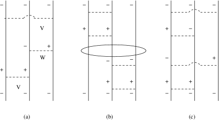
Figure 3: Third-order (a) and fourth-order ((b) and (c)) three-body diagrams discussed in the text. Diagram (b) is a folded diagram drawn in unfolded form for clarity.

Now directly from the matrix (12), or by explicitly drawing diagrams, the second order $\hat{Q}$-box is $3V^{2}/(-2\xi)$. Clearly the $W$ interaction can be incorporated to all orders yielding an exact $\hat{Q}$-box of $3V^{2}/(-2\xi-2W)$. The folded diagrams can then be included by differentiation as indicated in Eq. (2). In the approximation that we stop at order $V^{6}$ the interaction is

$$\langle V\rangle_{3} = -\frac{3V^{2}}{2(\xi+W)}+\frac{9V^{4}}{8(\xi+W)^{3}}-\frac{27V^{6}}{16(\xi+W)^{5}}$$ (14)

$$\equiv f_{3}(\xi)\;.$$

In order to disentangle the three-body interaction we need the two-body interaction for the state $|p_{1}-,p_{2}-\rangle$. Since this is only coupled to $|p_{1}+,p_{2}+\rangle$ by the Hamiltonian, the necessary matrix is $\left(\begin{array}[]{cc}-\xi&V\\ V&\xi\end{array}\right)$. For later use we note that the exact lowest eigenvalue is $\lambda_{-}^{(2)}=-\xi\sqrt{1+\frac{V^{2}}{\xi^{2}}}$. Now the exact $\hat{Q}$-box is $V^{2}/(-2\xi)$ and carrying out the folding to order $V^{6}$ as before

$$\langle V\rangle_{2}=-\frac{V^{2}}{2\xi}+\frac{V^{4}}{8\xi^{3}}-\frac{V^{6}}{16\xi^{5}}\equiv f_{2}(\xi)\;.$$ (15)

The one particle wavefunction is $a^{\dagger}_{p-}|0\rangle$ with energy $-{\textstyle{\frac{1}{2}}}\xi$ given by the unperturbed Hamiltonian $H_{0}$, so that the one-body interaction $V^{(1)}$ is zero. Thus, using Eq. (4) or (5), and noting that because of the degeneracy label $p$ there will only be three contributions from the two-body terms

$$\langle V^{(3)}\rangle=\langle V\rangle_{3}-3\langle V\rangle_{2}=\frac{3V^{2}W}{2\xi^{2}}+\frac{3V^{2}}{4\xi^{3}}(V^{2}-2W^{2})+\frac{3V^{2}W}{8\xi^{4}}(4W^{2}-9V^{2})-\frac{3V^{2}}{4\xi^{5}}(2V^{4}-9V^{2}W^{2}+2W^{4})\;.$$ (16)

Here we have expanded to sixth order in the interaction. Notice that there is no second-order contribution. This result can also be obtained by evaluating diagrams, for brevity we do not go beyond fourth order. In third order the diagram of Fig. 3(a) is required, while in fourth order the folded diagram of Fig. 3(b), drawn in unfolded form, and the non-folded diagram (c) are needed; by counting the number of independent diagrams of each type the numerical factors in Eq. (16) are obtained. If $W$ is set to zero in Eq. (16) the remaining three-body contributions come from folded diagrams, Fig. 3(b) and higher orders. The coefficients of the order $V^{4}$ and $V^{6}$ terms in Eq. (16) are larger than three times the corresponding values in Eq. (15). This supports the suggestion that even if non-folded three-body diagrams are small, three-body contributions arising from folding could be important.

We can, of course, obtain the exact three-body interaction for this simple Hamiltonian using the exact eigenvalues given. As we have remarked, the one-body interaction $V^{(1)}$ is zero. Then, subtracting the unperturbed energy, the two-body effective interaction is

$$\langle V^{(2)}\rangle=\xi\left(1-\sqrt{1+\frac{V^{2}}{\xi^{2}}}\right)\;.$$ (17)

The desired exact three-body interaction is therefore

$$\langle V^{(3)}\rangle=\lambda_{-}^{(3)}-3\langle V^{(2)}\rangle+{\textstyle{\frac{3}{2}}}\xi\;,$$ (18)

where the last term removes the contribution from $H_{0}$ in $\lambda_{-}^{(3)}$. Expanding this expression to sixth order of course yields Eq. (16) again. Notice that since $V^{(3)}$ depends on $W$ while $V^{(2)}$ does not, suitable adjustment of this parameter could yield a three-body interaction of magnitude comparable to the two-body interaction. For instance, in the limit $W\rightarrow\infty$ we have $V^{(3)}\rightarrow-3V^{(2)}$ since the eigenvalue is simply $-{\textstyle{\frac{3}{2}}}\xi$ in this case.

It is instructive to make the model a little more elaborate by changing the parameter $\xi$ of the one-body Hamiltonian to $\xi+\epsilon$. The first term is included in $H_{0}$ as before and $\epsilon$ is treated as a perturbation. The matrix (12) then becomes

$$\left(\begin{array}[]{cc}-{\textstyle{\frac{3}{2}}}\xi-{\textstyle{\frac{3}{2}}}\epsilon&\sqrt{3}V\\ \sqrt{3}V&{\textstyle{\frac{1}{2}}}\xi+{\textstyle{\frac{1}{2}}}\epsilon+2W\end{array}\right)\;.$$ (19)

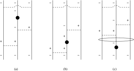
Figure 4: Fourth-order three-body diagrams discussed in the text. Diagram (c) is a folded diagram drawn in unfolded form for clarity and the dot represents a one-body insertion.

From the matrix directly, or by drawing diagrams, the $\hat{Q}$-box through second order contains both one- and two-body parts, namely $-{\textstyle{\frac{3}{2}}}\epsilon-3V^{2}/(2\xi)$. Starting in third order there will be diagrams with $\epsilon$ insertions. Since the intermediate state always involves two $+$ particles and one $-$ particle, the net insertion is $+{\textstyle{\frac{1}{2}}}\epsilon$ (note that valence unlinked contributions of the form of Fig. 2(d) occur here). If these insertions, together with the $W$ interactions are summed to all orders one obtains $-{\textstyle{\frac{3}{2}}}\epsilon-3V^{2}/(2\xi+2W+{\textstyle{\frac{1}{2}}}\epsilon)$, a result that can be obtained immediately from the matrix (19). Now an $\epsilon$ insertion on each of the three $-$ particles of the model space state $|1\rangle$ gives a net contribution of $-{\textstyle{\frac{3}{2}}}\epsilon$. If these insertions are folded out to all orders one obtains $-{\textstyle{\frac{3}{2}}}\epsilon-3V^{2}/(2\xi+2W+2\epsilon)$, in the process removing valence-unlinked diagrams. This result again follows immediately from the matrix (19). If this modified $\hat{Q}$-box is used in Eq. (2) to generate all the additional folded diagrams required we obtain $\langle V\rangle_{3}=-{\textstyle{\frac{3}{2}}}\epsilon+f_{3}(\xi+\epsilon)$. A similar procedure in the two-body case gives $\langle V\rangle_{2}=-\epsilon+f_{2}(\xi+\epsilon)$. In the one-body case $\langle V^{(1)}\rangle=-{\textstyle{\frac{1}{2}}}\epsilon$. Then using Eq. (4)

$$\langle V^{(3)}\rangle = \langle V\rangle_{3}-3\langle V\rangle_{2}+3\langle V^{(1)}\rangle$$ (20)

$$= \frac{3V^{2}W}{2\xi^{2}}+\frac{3V^{2}}{4\xi^{3}}(V^{2}-2W^{2}-4\epsilon W)+\frac{3V^{2}}{8\xi^{4}}(4W^{3}-9V^{2}W-6V^{2}\epsilon+12W^{2}\epsilon+12W\epsilon^{2})$$

$$-\frac{3V^{2}}{4\xi^{5}}(2V^{4}-9V^{2}W^{2}+2W^{4}-18V^{2}W\epsilon+8W^{3}\epsilon-6V^{2}\epsilon^{2}+12W^{2}\epsilon^{2}+8W\epsilon^{3})\;,$$

to sixth order in the interaction. Obviously the terms which do not involve $\epsilon$ are the same as in Eq. (16). Notice that terms of the form $V^{2}\epsilon^{n}/\xi^{n+1}$ necessarily belong to the two-body interaction and do not occur here. The fourth order term involving $\epsilon$ is generated from the diagrams of Fig. 4(a) and (b), as well as the folded diagram (c). Here $V^{(1)}$ is represented by a dot. Each diagram stands for several different diagrams of the same general structure and the coefficient in Eq. (20) is obtained by accounting for all of them. The result in Eq. (20) can also be obtained by a power series expansion of the exact result which is the analogue of Eq. (18), namely

$$\langle V^{(3)}\rangle=\lambda_{-}^{(3)}-3\langle V^{(2)}\rangle-3\langle V^{(1)}\rangle+{\textstyle{\frac{3}{2}}}\xi\;,$$ (21)

with the replacement $\xi\rightarrow\xi+\epsilon$ being made in the first two terms on the right.

III.2 The Case $U\neq 0$

Here we take the model space to consist of states $|1\rangle$ and $|2\rangle$ of Eq. (10) and require our effective interaction to reproduce two of the eigenvalues of the matrix (11). It is simplest to work with a degenerate model space and we choose the unperturbed energy to be $-{\textstyle{\frac{3}{2}}}\xi$. The remainder of the diagonal $(2,2)$ contribution in (11) is then included as a perturbation. The lowest order $\hat{Q}$-box of a given type is easily written down as discussed in Sec. III.1. Here we also need to account for multiple scatterings back and forth between states $|3\rangle$ and $|4\rangle$ which is easily done by summing the infinite series. Thus we can obtain the exact $\hat{Q}$-box:

$$\langle 1|\hat{Q}|1\rangle=\frac{3V^{2}}{-2\xi-2W+U^{2}/\xi}\;,$$

$$\langle 2|\hat{Q}|1\rangle=\langle 1|\hat{Q}|2\rangle=\sqrt{3}U+\frac{2\sqrt{3}UV}{-2\xi-2W+U^{2}/\xi}$$

$$\qquad\qquad\qquad\qquad\ \ +\frac{\sqrt{3}UV^{2}}{2\xi(\xi+W)-U^{2}}\;,$$

$$\langle 2|\hat{Q}|2\rangle=\xi+2W+\frac{4U^{2}}{-2\xi-2W+U^{2}/\xi}$$

$$\quad+\frac{V^{2}}{-\xi+U^{2}/(2\xi+2W)}+\frac{4VU^{2}}{2\xi(\xi+W)-U^{2}}\;.$$ (22)

Insertion of this in Eq. (2) will yield an effective interaction which reproduces two of the exact eigenvalues. This is illustrated by the solid lines in Fig. 5. We work in units of $\xi$ and have chosen the dimensionless ratios $V/\xi=W/\xi=-0.4$ and $U/\xi=-0.15$. The label 0 fold in Fig. 5 implies that the solid lines are obtained from the $\hat{Q}$-box alone, while the labelling $n$ fold implies that the summation over $m$ in Eq. (2) extends to $m=n$. As $n$ is increased so that more folded diagrams are included the eigenvalues of the effective interaction converge to the exact result. The deviations are less than 0.2% by the time $n=5$.

Figure 5: Comparison of the eigenvalues (in units of $\xi$) of the effective interaction with $n$ folds to the exact result. For the solid lines two- and three-body interactions are included, while for the dashed lines only two-body interactions are considered.

This analysis necessarily includes effective three-body interactions and we would like to assess the effect of their removal. To that end consider first the two-body problem. We only need to consider the $J=1$ matrix which is

$$\left(\begin{array}[]{ccc}-\xi&U/\sqrt{2}&V\\ U/\sqrt{2}&W&U/\sqrt{2}\\ V&U/\sqrt{2}&\xi\end{array}\right)\;,$$ (23)

in the basis

$$|a\rangle \equiv |J=1J_{z}=-1\rangle=|p_{1}-,p_{2}-\rangle\;,$$

$$|b\rangle \equiv |J=1J_{z}=0\rangle=\bigl{\{}|p_{1}-,p_{2}+\rangle+|p_{1}+,p_{2}-\rangle\bigr{\}}/\sqrt{2}\;,$$

$$|c\rangle \equiv |J=1J_{z}=+1\rangle=|p_{1}+,p_{2}+\rangle\;.$$ (24)

Taking the model space to comprise states $|a\rangle$ and $|b\rangle$ and choosing degenerate unperturbed energies of $-\xi$, the exact $\hat{Q}$-box is

$$\langle a|\hat{Q}|a\rangle = -\frac{V^{2}}{2\xi}\;,$$

$$\langle b|\hat{Q}|a\rangle = \langle a|\hat{Q}|b\rangle=\frac{U}{\sqrt{2}}-\frac{VU}{2\sqrt{2}\xi}\;,$$

$$\langle b|\hat{Q}|b\rangle = \xi+W-\frac{U^{2}}{4\xi}\;.$$ (25)

Figure 6: A three-body diagram discussed in the text.

When used in Eq. (2) this will give an effective interaction which yields two of the exact two-body eigenvalues. However our interest is in using this in the three particle case. The $(a,a)$ element will contribute thrice to the $(1,1)$ component of the three body $\hat{Q}$-box and once to the $(2,2)$ case. Note that for the latter the use of $-{\textstyle{\frac{3}{2}}}\xi$ for the unperturbed energies requires that the energy denominator be modified to $3\xi$. This can be viewed as arising from diagrams with a one-body insertions of $-\xi$ folded out to all orders to correct the energy of the model space $+$ state. The two-body part of the $(b,b)$ element contributes twice to the $(2,2)$ component; the one-body part is associated with the single $+$ state and therefore only contributes once. Finally the $(b,a)$ element contributes thrice to the $(2,1)$ component multiplied by a factor $\sqrt{{\textstyle{\frac{2}{3}}}}$ due to the normalization in Eqs. (10) and (24). In this way the one- plus two-body contribution to the three-body $\hat{Q}$-box is found to be

$$\langle 1|\hat{Q}|1\rangle = -\frac{3V^{2}}{2\xi}\;,$$

$$\langle 2|\hat{Q}|1\rangle = \langle 1|\hat{Q}|2\rangle=\sqrt{3}U-\frac{\sqrt{3}VU}{2\xi}\;,$$

$$\langle 2|\hat{Q}|2\rangle = \xi+2W-\frac{U^{2}}{2\xi}-\frac{V^{2}}{3\xi}\;.$$ (26)

Note a subtlety here. A diagram of the type shown in Fig. 6 might appear to be a two-body contribution to the three-particle interaction. However if the non-interacting line is erased the remainder cannot contribute to the two-body interaction because the intermediate state is in the model space. This is no longer the case with three particles present where the intermediate state lies outside the model space, thus it is properly counted as a three-body interaction. Comparing Eq. (26) to Eq. (22) we see that here the three-body interactions begin at second order due to the presence of state $|2\rangle$. Using the two-body approximation of Eq. (26) for the $\hat{Q}$-box in Eq. (2) yields the eigenvalues denoted by dashed lines in Fig. 5. Comparison with the exact result shows that the two-body approximation converges more rapidly in terms of the number of folds, but the converged result has a lower (upper) eigenvalue which is in error by 9% (4%); this is not insignificant. The point is also made in Fig. 7 where the same values of $V/\xi$ and $U/\xi$ are used, but the parameter $W/\xi$ is allowed to vary. Again the solid line employs an effective interaction with one-, two- and three-body terms, while the dashed line is obtained when the three-body contributions are omitted. Clearly the accuracy of the two-body approximation is dependent on the precise values of the parameters used. In this example it can be quite accurate for one of the eigenvalues for particular values of $W/\xi$, but then it is inaccurate for the other eigenvalue.

Figure 7: Eigenvalues (in units of $\xi$) obtained with the two-body effective interaction (dashed curves) compared with the exact values (solid curves), as a function of $w/\xi$.

IV Concluding remarks

We have shown how the effective three-body interaction may be isolated from the nonfolded and folded diagrams generated from a $\hat{Q}$-box which contains one-, two- and three-body terms. In order to gain some insight this was applied to the Lipkin model where exact results can easily be obtained. Even for this simple example subtle points arose. Numerically we showed that for a system of three particles the three-body components of the effective interaction cannot be assumed to be negligible. Interestingly in our effective $2\times 2$ matrix example the two-body interaction alone sometimes gave quite an accurate result for one of the eigenvalues, but then the other was rather inaccurate.

This suggests that the role of three-body interactions in realistic situations deserves further study, in particular in medium-heavy and heavy nuclei. As mentioned in the Introduction we hope to carry out such a study for the entire range of Sn isotopes using the formalism discussed here. The difficulty in explaining the trend of the binding energies is a particular motivation, but more important is the fact that three-body effects scale with the number of valence particles cubed, while two-body contributions scale with the square. Thus an examination of some thirty Sn isotopes should allow a rather definitive assessment of the role of three-body interactions to be made.

- (1) A. Polls, H. Müther, A. Faessler, T. T. S. Kuo, and E. Osnes, Nucl. Phys. A401, 124 (1983).
- (2) H. Müther, A. Polls, and T. T. S. Kuo, Nucl. Phys. A435, 548 (1985).
- (3) P. K. Rath, A. Faessler, H. Müther, and A. Watt, Nucl. Phys. A492, 127 (1989).
- (4) D. J. Dean, T. Engeland, M. Hjorth-Jensen, M. P. Kartamyshev, and E. Osnes, Prog. Part. Nucl. Phys. 53, 419 (2004).
- (5) A. P. Zuker, Phys. Rev. Lett. 90, 042502 (2003).
- (6) M. Homna, T. Otsuka, B. A. Brown, and T. Mizusaki, Phys. Rev. C 69, 034335 (2004).
- (7) T. Otsuka, M. Homna, T. Mizusaki, N. Shimizu, and Y. Utsuno, Prog. Part. Nucl. Phys. 47, 319 (2001).
- (8) B. A. Brown, Prog. Part. Nucl. Phys. 47, 517 (2001), and references therein.
- (9) M. Hjorth-Jensen, T. T. S. Kuo, and E. Osnes, Phys. Rep. 261, 125 (1995).
- (10) M. Lipoglavšek et al., Phys. Rev. C 65, 021302(R) (2002).
- (11) M. Lipoglavšek et al., Phys. Rev. C 65, 051307(R) (2002).
- (12) M. Lipoglavšek et al., Phys. Rev. C 66, 011302(R) (2002).
- (13) T. Engeland, M. Hjorth-Jensen, and E. Osnes, Phys. Rev. C 61, 021302(R) (2000).
- (14) J. J. Ressler, W. B. Walters, C. N. Davids, D. J. Dean, A. Heinz, M. Hjorth-Jensen, D. Seweryniak, and J. Shergur, Phys. Rev. C 66, 024308 (2002).
- (15) A. Holt, T. Engeland, M. Hjorth-Jensen, and E. Osnes, Nucl. Phys. A634, 41 (1998).
- (16) S. C. Pieper, V. R. Pandharipande, R. B. Wiringa, and J. Carlson, Phys. Rev. C 64, 014001 (2001).
- (17) S. C. Pieper, K. Varga, and R. B. Wiringa, Phys. Rev. C 66, 0044310 (2002).
- (18) R. B. Wiringa and S. C. Pieper, Phys. Rev. Lett. 89, 182501 (2002).
- (19) P. Navrátil and W. E. Ormand, Phys. Rev. Lett. 88, 152502 (2002).
- (20) P. Navrátil and W. E. Ormand, Phys. Rev. C 68, 034305 (2003).
- (21) T. T. S. Kuo and E. Osnes, Folded-diagram Theory of the Effective Interaction in Atomic Nuclei, Springer Lecture Notes in Physics (Springer, Berlin, 1990) Vol. 364; T. T. S. Kuo, Lecture notes in Physics; Topics in Nuclear Physics, eds. T. T. S. Kuo and S. S. M. Wong, (Springer, Berlin, 1981) Vol. 144, p. 248.
- (22) I. Talmi, Simple Models of Complex Nuclei, Contemporary Concepts in Physics (Harwood Academic Publishers, Chur, Switzerland, 1993) Vol. 7.
- (23) K. Kowalski, D. J. Dean, M. Hjorth-Jensen, T. Papenbrock, and P. Piecuch, Phys. Rev. Lett. 92, 132501 (2004).
- (24) H. J. Lipkin, N. Meshkov, and A. J. Glick, Nucl. Phys. 62, 188 (1965).
- (25) K. J. Abraham and J. P. Vary, preprint nucl-th/0410037.
- (26) B. H. Brandow, Rev. Mod. Phys. 39, 771 (1967).
- (27) P. J. Ellis and E. Osnes, Rev. Mod. Phys. 49, 777 (1977).
- (28) K. Suzuki, R. Okamoto, P. J. Ellis, and T. T. S. Kuo, Nucl. Phys. A567, 576 (1994).