Exotic dark matter together with dark energy or cosmological constant seem to dominate in the Universe. An even higher density of such matter seems to be gravitationally trapped in our Galaxy. The nature of dark matter can be unveiled only, if it is detected in the laboratory. Thus the accomplishment of this task is central to physics and cosmology. Current fashionable supersymmetric models provide a natural dark matter candidate, which is the lightest supersymmetric particle (LSP). Such models combined with fairly well understood physics like the quark substructure of the nucleon can yield the effective transition operator at the nucleon level. We know, however, that the LSP is much heavier than the proton, while its average energy is in the keV region. Thus the most likely possibility for its direct detection is via its elastic scattering with a nuclear target by observing the recoiling nucleus. In order to evaluate the event rate one needs the nuclear structure (form factor and/or spin response function) for the special nuclear targets of experimental interest. Since the expected rates for neutralino-nucleus scattering are expected to be small, one should exploit all the characteristic signatures of this reaction. Such are: (i) In the standard recoil measurements the modulation of the event rate due to the Earth’s motion. (ii) In directional recoil experiments the correlation of the event rate with the sun’s motion. One now has both modulation, which is much larger and depends not only on time, but on the direction of observation as well, and a large forward-backward asymmetry. (iii) In non recoil experiments gamma rays following the decay of excited states populated during the Nucleus-LSP collision. Branching ratios of about 6 percent are possible. (iv) novel experiments in which one observes the electrons prod used during the collision of the LSP with the nucleus. Branching ratios of about 10 per cent are possible.

1 Introduction

One of the greatest discoveries of the last couple of decays is the realization that the matter, which can shine, constitutes a very small fraction of the universe. The universe is composed primarily of dark matter and dark energy, which are incapable of emitting light. If one defines $\Omega_{i}=\frac{\rho_{i}}{\rho_{c}}$ for the species $i$, where $\rho_{c}$ the critical density (see sec. 2), the recent cosmological observations [1], when combined, lead to:

$$\Omega_{b}=0.05,\Omega_{CDM}=0.30,\Omega_{\Lambda}=0.65$$

for ordinary matter, dark matter and dark energy respectively. Their sum is [1] $\Omega=1.11\pm 0.07$, i.e. unity within the experimental errors , which means that the universe is flat.

Additional indirect information comes from the rotational curves [2]. The rotational velocity of an object increases so long is surrounded but matter. Once outside matter the velocity of rotation drops as the square root of the distance. Such observations are not possible in our own galaxy. The observations of other galaxies, similar to our own, indicate that the rotational velocities of objects outside the luminous matter do not drop (see Fig. 1). So there must be a halo of dark matter out there.

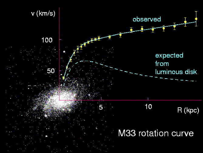
Figure 1.  : The rotational velocity distance. Clearly it does not fall outside the luminous matter. This is suggestive of the presence of a dark matter halo outside the M33 galaxy.

As we have already mentioned, however, it is only the direct detection of dark matter in the laboratory, which will unravel the nature of the constituents of dark matter. In fact one such experiment, the DAMA, has claimed the observation of such signals, which with better statistics has subsequently been interpreted as modulation signals [3]. These data, however, if they are due to the coherent process, are not consistent with other recent experiments, see e.g. EDELWEISS and CDMS [4].
Supersymmetry naturally provides candidates for the dark matter constituents. In the most favored scenario of supersymmetry the LSP can be simply described as a Majorana fermion (LSP or neutralino), a linear combination of the neutral components of the gauginos and higgsinos [6]-[9]. We are not going to address issues related to SUSY in this paper. Most SUSY models predict nucleon cross sections much smaller the the present experimental limit $\sigma_{S}\leq 10^{-5}pb$ for the coherent process. As we shall see below the constraint on the spin cross-sections is less stringent.

Since the neutralino is expected to be non relativistic with average kinetic energy $<T>\approx 40KeV(m_{\chi}/100GeV)$, it can be directly detected mainly via the recoiling of a nucleus (A,Z) in elastic scattering.

In some rare instances the low lying excited states may also be populated [11]. In this case one may observe the emitted $\gamma$ rays. Finally it has also recently been suggested [23] that one may be able to detect the neutralino by observing the ionization electrons produced during its collision with the nucleus.

In every case to extract from the data information about SUSY from the relevant nucleon cross section, one must know the relevant nuclear matrix elements [12]-[13]. The static spin matrix elements used in the present work have been obtained from the literature [11].

Anyway since in all types of experiments the obtained rates are very low, one would like to be able to exploit the modulation of the event rates due to the earth’s revolution around the sun [14],[15]. In order to accomplish this one adopts a folding procedure, i.e one has to assume some velocity distribution [14, 15, 17, 18] for the LSP. One also would like to exploit other signatures expected to show up in directional experiments [19]. This is possible, since the sun is moving with relatively high velocity with respect to the center of the galaxy.

2 Matter Density Versus Cosmological Constant (Dark Energy).

As we have mentioned in the previous section the universe is primarily made of dark matter and dark energy. The nature of each one of them is not presently known. We hope the future experiments to shed light on this. The future of the universe depends on the composition and the nature of these two constituents. In the present case we will briefly explore the possibility that the dark energy density is constant, independent of the size of the universe, i.e. it coincides with Einstein’s cosmological constant.

The evolution of the Universe is governed by the General Theory of Relativity. The most commonly used model is that of Friedman, which utilizes the Robertson- Walker metric

$$(ds)^{2}=(dt)^{2}-a^{2}(t)[\frac{(dr)^{2}}{1-\kappa r^{2}}+r^{2}((d\theta)^{2}+\sin^{2}\theta(d\phi)^{2})]$$ (1)

, where $a(t)$ is the scale factor. The resulting Einstein equations are:

$$R_{\mu\nu}-\frac{1}{2}g_{\mu\nu}R=-8\pi G_{N}T_{\mu\nu}+\Lambda g_{\mu\nu}$$ (2)

where $G_{N}$ is Newton’s constant and $\Lambda$ is the cosmological constant. The equation for the scale factor $a(t)$ becomes:

$$\frac{d^{2}a}{dt^{2}}=-\frac{4\pi}{3}G_{N}(\rho+3p)a=-\frac{4\pi G_{N}\rho}{3}a+\frac{\Lambda}{3}$$ (3)

where $\rho$ is the mass density. Then the energy is

$$E=\frac{1}{2}m(\frac{ar}{dt})^{2}-G_{N}\frac{m}{a}(4\pi\rho a^{3})+\frac{\Lambda}{6}ma^{2}=constant=-\frac{\kappa}{2}m$$ (4)

This can be equivalently be written as

$$H^{2}+\frac{\kappa}{a^{2}}=\frac{8\pi}{3}G_{N}\rho+\frac{\Lambda}{3}$$ (5)

where the quantity $H$ is Hubble’s constant defined by

$$H=\frac{1}{a}\frac{da}{dt}$$ (6)

Hubble’s constant is perhaps the most important parameter of cosmology. In fact it is not a constant but it changes with time. Its present day value is given by

$$H_{0}=(65\pm 15)~{}km/s~{}M_{pc}^{-1}$$ (7)

In other words $H_{0}^{-1}=(1.50\pm).35)\times 10^{10}~{}y$, which is roughly equal to the age of the Universe. Astrophysicists conventionally write it as

$$H_{0}=100~{}h~{}km/s~{}M_{pc}^{-1}~{}~{}~{}~{},~{}~{}~{}~{}~{}0.5<h<0.8$$ (8)

Equations 3-5 coincide with those of the Newtonian theory with the following two types of forces: An attractive force decreasing in absolute value with the scale factor (Newton) and a repulsive force increasing with the scale factor (Einstein):

$$F=-G_{N}\frac{mM}{a^{2}}~{}~{}(Newton)~{}~{},~{}~{}F=\frac{1}{3}\Lambda ma~{}~{}(Einstein)$$ (9)

Historically the cosmological constant was introduced by Einstein so that General Relativity yields a stationary Universe, i.e. one which satisfies the conditions:

$$\frac{da}{dt}=0~{}~{}~{}~{}\frac{d^{2}a}{dt^{2}}=0$$ (10)

Indeed for $\kappa>0$, the above equations lead to $a=a_{c}$=constant provided that

$$\frac{1}{3}\Lambda a_{c}-\frac{4\pi}{3}G_{N}\rho a{c}=0~{}~{},~{}~{}\frac{1}{3}\Lambda a^{2}_{c}-\frac{4\pi}{3}G_{N}\rho a^{2}_{c}=\kappa$$ (11)

These equations have a non trivial solution provided that the density $\rho$ and the cosmological constant $\Lambda$ are related, i.e.

$$\Lambda=4\pi G_{N}\rho$$ (12)

The radius of the Universe then is given by

$$a_{c}=[\frac{\kappa}{4\pi G_{N}\rho}]^{1/2}$$ (13)

In our days we do not believe that the universe is static. So the two parameters, density and cosmological constant, need not be related. Define now

$$\Omega_{m}=\frac{\rho}{\rho_{c}}~{}~{},~{}~{}\Omega_{\Lambda}=\frac{\rho_{v}}{\rho_{c}}~{}~{},~{}~{}\rho_{v}=\frac{\Lambda}{8\pi G_{N}}~{}~{}("vacuum"density)$$ (14)

The critical density is

$$\rho_{c}=1.8\times 10^{-23}h^{2}\frac{g}{cm^{3}}=10h^{2}\frac{nucleons}{m^{3}}$$ (15)

With these definitions Friedman’s equation $E=-\kappa\frac{m}{2}$ takes the form

$$\frac{\kappa}{a^{2}}=(\Omega_{m}+\Omega_{\Lambda}-1)H^{2}$$ (16)

Thus we distinguish the following special cases:

$$\kappa>0~{}~{}~{}~{}\Leftrightarrow~{}~{}~{}~{}\Omega_{m}+\Omega_{\Lambda}>1~{}~{}~{}~{}\Leftrightarrow Closed~{}curved~{}Universe$$ (17)

$$\kappa=0~{}~{}~{}~{}\Leftrightarrow~{}~{}~{}~{}\Omega_{m}+\Omega_{\Lambda}=1~{}~{}~{}~{}\Leftrightarrow Open~{}Flat~{}Universe$$ (18)

$$\kappa<0~{}~{}~{}~{}\Leftrightarrow~{}~{}~{}~{}\Omega_{m}+\Omega_{\Lambda}<1~{}~{}~{}~{}\Leftrightarrow Open~{}Curved~{}Universe$$ (19)

In other words it is the combination of matter and ”vacuum” energy, which determines the fate of the our Universe.

To proceed further and obtain $a(t)$ we need an equation of state, which relates the pressure and the density. This of the form:

$$p=w\rho c^{2}$$

the one finds

$$a(t)=const~{}t^{2/(3(1+w))}~{}~{},~{}~{}\frac{\ddot{a}(t)}{a(t)}=-\frac{4\pi G_{N}}{3}(1+3w)\rho$$ (20)

We thus see that we have acceleration if $w<-1/3$ and deceleration otherwise. The following cases are of interest:

• $w=1/3$. This corresponds to a universe dominated by radiation

• $w=0$. This corresponds to a universe dominated by non relativistic matter.

• $w=-1$. This means that the cosmological constant is dominant. In this case the Hubble parameter is a constant and $a(t)=a_{0}e^{H_{0}t}$.

• $-1<w<-1/3$. This corresponds to dark energy.

We are not going to elaborate further on this issue. The observational situation at present is summarized in Fig. 2.

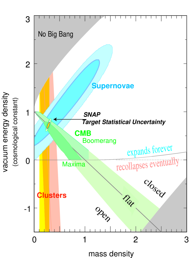
Figure 2.  : The allowed region in the $\Omega_{m}$, $\Omega_{DE}$, with $m$ indicating all matter and $DE$ the dark energy, for the various experiments indicated on the plot.

3 Rates

The differential non directional rate can be written as

$$dR_{undir}=\frac{\rho(0)}{m_{\chi}}\frac{m}{Am_{N}}d\sigma(u,\upsilon)|{\boldmath\upsilon}|$$ (21)

where $d\sigma(u,\upsilon)$ was given above, $\rho(0)=0.3GeV/cm^{3}$ is the LSP density in our vicinity, m is the detector mass and $m_{\chi}$ is the LSP mass

The directional differential rate, in the direction $\hat{e}$ of the recoiling nucleus, is:

$$dR_{dir}=\frac{\rho(0)}{m_{\chi}}\frac{m}{Am_{N}}|\upsilon|\hat{\upsilon}.\hat{e}~{}\Theta(\hat{\upsilon}.\hat{e})~{}\frac{1}{2\pi}~{}d\sigma(u,\upsilon\ \delta(\frac{\sqrt{u}}{\mu_{r}\upsilon\sqrt{2}}-\hat{\upsilon}.\hat{e})$$

where $\Theta(x)$ is the Heaviside function and:

$$d\sigma(u,\upsilon)==\frac{du}{2(\mu_{r}b\upsilon)^{2}}[(\bar{\Sigma}_{S}F(u)^{2}+\bar{\Sigma}_{spin}F_{11}(u)]$$ (22)

where $u$ the energy transfer $Q$ in dimensionless units given by

$$u=\frac{Q}{Q_{0}}~{}~{},~{}~{}Q_{0}=[m_{p}Ab]^{-2}=40A^{-4/3}~{}MeV$$ (23)

with $b$ is the nuclear (harmonic oscillator) size parameter. $F(u)$ is the nuclear form factor and $F_{11}(u)$ is the spin response function associated with the isovector channel. It is the area of constructing such form factors and momentum distributions that Professor M. Grypeos, honored in this volume, has made a great contribution [20].

The scalar cross section is given by:

$$\bar{\Sigma}_{S}=(\frac{\mu_{r}}{\mu_{r}(p)})^{2}\sigma^{S}_{p,\chi^{0}}A^{2}\left[\frac{1+\frac{f^{1}_{S}}{f^{0}_{S}}\frac{2Z-A}{A}}{1+\frac{f^{1}_{S}}{f^{0}_{S}}}\right]^{2}\approx\sigma^{S}_{N,\chi^{0}}(\frac{\mu_{r}}{\mu_{r}(p)})^{2}A^{2}$$ (24)

(since the heavy quarks dominate the isovector contribution is negligible). $\sigma^{S}_{N,\chi^{0}}$ is the LSP-nucleon scalar cross section. The spin Cross section is given by:

$$\bar{\Sigma}_{spin}=(\frac{\mu_{r}}{\mu_{r}(p)})^{2}\sigma^{spin}_{p,\chi^{0}}~{}\zeta_{spin},\zeta_{spin}=\frac{1}{3(1+\frac{f^{0}_{A}}{f^{1}_{A}})^{2}}S(u)$$ (25)

$$S(u)\approx S(0)=[(\frac{f^{0}_{A}}{f^{1}_{A}}\Omega_{0}(0))^{2}+2\frac{f^{0}_{A}}{f^{1}_{A}}\Omega_{0}(0)\Omega_{1}(0)+\Omega_{1}(0))^{2}\,]$$ (26)

Some static of interest to the planned experiments are given in table 1. The shown results are obtained from DIVARI [13], Ressel and Dean (*) [12], the Finish group (**) [16] and the Ioannina team (+) [5], [10].

TABLE 1.  : The static spin matrix elements for various nuclei. For light nuclei the calculations are from DIVARI. For ${}^{127}I$ the results presented are from Ressel and Dean (*) and the Finish group (**). For ${}^{207}Pb$ they were obtained by the Ioannina team (+).

	19F	29Si	23Na	${}^{127}I^{*}$	${}^{127}I^{**}$	${}^{207}Pb^{+}$
$[\Omega_{0}(0)]^{2}$	2.610	0.207	0.477	3.293	1.488	0.305
$[\Omega_{1}(0)]^{2}$	2.807	0.219	0.346	1.220	1.513	0.231
$\Omega_{0}(0)\Omega_{1}(0)$	2.707	-0.213	0.406	2.008	1.501	-0.266
$\mu_{th}$	2.91	-0.50	2.22
$\mu_{exp}$	2.62	-0.56	2.22
$\frac{\mu_{th}(spin)}{\mu_{exp}}$	0.91	0.99	0.57

$f^{0}_{A}$, $f^{1}_{A}$ are the isoscalar and the isovector axial current couplings at the nucleon level obtained from the corresponding ones given by the SUSY models at the quark level, $f^{0}_{A}(q)$, $f^{1}_{A}(q)$, via renormalization coefficients $g^{0}_{A}$, $g_{A}^{1}$, i.e. $f^{0}_{A}=g_{A}^{0}f^{0}_{A}(q),f^{1}_{A}=g_{A}^{1}f^{1}_{A}(q).$ These couplings and the associated nuclear matrix elements are normalized so that, for the proton at $u=0$, yield $\zeta_{spin}=1$. If the nuclear contribution comes predominantly from protons ($\Omega_{1}=\Omega_{0}=\Omega_{p}$), $S(u)\approx\Omega_{p}^{2}$ and one can extract from the data the proton cross section. If the nuclear contribution comes predominantly from neutrons (($\Omega_{0}=-\Omega_{1}=\Omega_{n}$) one can extract the neutron cross section. In many cases, however, one can have contributions from both protons and neutrons. The situation is then complicated, but it turns out that $g^{0}_{A}=0.1~{}~{},~{}~{}g^{1}_{A}=1.2$ Thus the isoscalar amplitude is suppressed, i.e $S(0)\approx\Omega^{2}_{1}$. Then the proton and the neutron spin cross sections are the same.

4 Results

To obtain the total rates one must fold with LSP velocity and integrate the above expressions over the energy transfer from $Q_{min}$ determined by the detector energy cutoff to $Q_{max}$ determined by the maximum LSP velocity (escape velocity, put in by hand in the Maxwellian distribution), i.e. $\upsilon_{esc}=2.84~{}\upsilon_{0}$ with $\upsilon_{0}$ the velocity of the sun around the center of the galaxy($229~{}Km/s$).

4.1 Non directional rates

Ignoring the motion of the Earth the total non directional rate is given by

$$R=\bar{K}\left[c_{coh}(A,\mu_{r}(A))\sigma_{p,\chi^{0}}^{S}+c_{spin}(A,\mu_{r}(A))\sigma_{p,\chi^{0}}^{spin}~{}\zeta_{spin}\right]$$ (27)

where $\bar{K}=\frac{\rho(0)}{m_{\chi^{0}}}\frac{m}{m_{p}}~{}\sqrt{\langle v^{2}\rangle}$ and

$$c_{coh}(A,\mu_{r}(A))=\left[\frac{\mu_{r}(A)}{\mu_{r}(p)}\right]^{2}A~{}t_{coh}(A)~{},c_{spin}(A,\mu_{r}(A))=\left[\frac{\mu_{r}(A)}{\mu_{r}(p)}\right]^{2}\frac{t_{spin}(A)}{A}$$ (28)

where $t$ is the modification of the total rate due to the folding and nuclear structure effects. It depends on $Q_{min}$, i.e. the energy transfer cutoff imposed by the detector and $a=[\mu_{r}b\upsilon_{0}\sqrt{2}]^{-1}$ The parameters $c_{coh}(A,\mu_{r}(A))$, $c_{spin}(A,\mu_{r}(A))$, which give the relative merit for the coherent and the spin contributions in the case of a nuclear target compared to those of the proton, are tabulated in table 2 for energy cutoff $Q_{min}=0,~{}10$ keV. Via Eq. (27) we can extract the nucleon cross section from the data.

Using $\Omega^{2}_{1}=1.22$ and $\Omega^{2}_{1}=2.8$ for ¹²⁷I and ¹⁹F respectively the extracted nucleon cross sections satisfy:

$$\frac{\sigma^{spin}_{p,\chi^{0}}}{\sigma^{S}_{p,\chi^{0}}}=\left[\frac{c_{coh}(A,\mu_{r}(A))}{c_{spin}(A,\mu_{r}(A))}\right]\frac{3}{\Omega^{2}_{1}}\Rightarrow\approx\times 10^{4}~{}(A=127)~{},~{}\approx\times 10^{2}~{}(A=19)$$ (29)

It is for this reason that the limit on the spin proton cross section extracted from both targets is much poorer. For heavy LSP, $\geq 100$ GeV, due to the nuclear form factor, $t_{spin}(127)<t_{spin}(19)$. This disadvantage cannot be overcome by the larger reduced mass. It even becomes worse, if the effect of the spin ME is included. For the coherent process, however, the light nucleus is no match (see Table 2).

TABLE 2.  : The factors $c19=c_{coh}(19,\mu_{r}(19))$, $s19=c_{spin}(19,\mu_{r}(19))$ and $c127=c_{coh}(127,\mu_{r}(127))$, $s127=c_{spin}(127,\mu_{r}(127))$ for two values of $Q_{min}$.

$Q_{min}$		$m_{\chi}$ (GeV)
keV		20	30	40	50	60	80	100	200
0	c19	2080	2943	3589	4083	4471	5037	5428	6360
0	s19	5.7	8.0	9.7	10.9	11.9	13.4	14.4	16.7
0	c127	37294	63142	84764	101539	114295	131580	142290	162945
0	s127	2.2	3.7	4.9	5.8	6.5	7.6	8.4	10.4
10	c19	636	1314	1865	2302	2639	3181	3487	4419
10	s19	1.7	3.5	4.9	6.0	6.9	8.3	9.1	11.4
10	c127	0	11660	24080	36243	45648	58534	69545	83823
10	s127	0	0.6	1.3	1.9	2.5	3.3	4.0	5.8

If the effects of the motion of the Earth around the sun are included, the total non directional rate is given by

$$R=\bar{K}\left[c_{coh}(A,\mu_{r}(A))\sigma_{p,\chi^{0}}^{S}(1+h(a,Q_{min})cos{\alpha})\right]$$ (30)

and an analogous one for the spin contribution. $h$ is the modulation amplitude and $\alpha$ is the phase of the Earth, which is zero around June 2nd, see Fig 3.

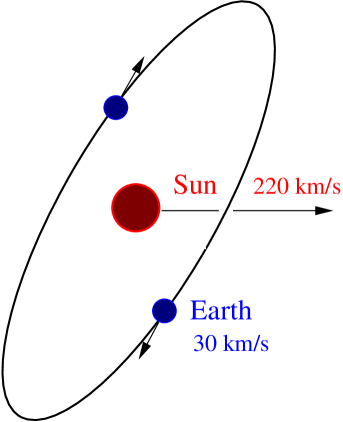
Figure 3.  : The motion of the earth around the sun. The sun is moving with a velocity in the plane of the galaxy, which is perpendicular to the page.

The modulation amplitude would be an excellent signal in discriminating against background, but unfortunately it is very small, less than two per cent. Furthermore for intermediate and heavy nuclei, it can even change sign for sufficiently heavy LSP (see Fig. 4). So in our opinion a better signature is provided by directional experiments, which measure the direction of the recoiling nucleus.

$h\rightarrow$

$h\rightarrow$

$m_{LSP}\rightarrow$ (GeV)

Figure 4.  : The modulation amplitude $h$ as a function of the LSP mass in the case of ¹²⁷I for $Q_{min}=0$ on the left and $Q_{min}=10$ keV on the right.

4.2 Directional Rates.

Since the sun is moving around the galaxy in a directional experiment, i.e. one in which the direction of the recoiling nucleus is observed, one expects a strong correlation of the event rate with the motion of the sun. In fact the directional rate can be written as:

$$R_{dir}=\frac{\kappa}{2\pi}\bar{K}\left[c_{coh}(A,\mu_{r}(A))\sigma_{p,\chi^{0}}^{S}(1+h_{m}cos{(\alpha-\alpha_{m}~{}\pi)})\right]$$ (31)

and an analogous one for the spin contribution. The modulation now is $h_{m}$, with a shift $\alpha_{m}\pi$ in the phase of the Earth $\alpha$, depending on the direction of observation. $\kappa/(2\pi)$ is the reduction factor of the unmodulated directional rate relative to the non-directional one. The parameters $\kappa~{},~{}h_{m}~{},~{}\alpha_{m}$ strongly depend on the direction of observation.

Figure 5.  : The expected modulation amplitude $h_{m}$ for $A=127$ in a direction outward from the galaxy on the left and perpendicular to the galaxy on the right as a function of the polar angle measured from the sun’s velocity. For angles than $\pi/2$ it is irrelevant since the event rates are tiny.

We prefer to use the parameters $\kappa$ and $h_{m}$, since, being ratios, are expected to be less dependent on the parameters of the theory. In the case of $A=127$ we exhibit the the angular dependence of $h_{m}$ for an LSP mass of $m_{\chi}=100GeV$ in Fig. 5. We also exhibit the parameters $t$, $h$, $\kappa,h_{m}$ and $\alpha_{m}$ for the target $A=19$ in Table 3 (for the other light systems the results are almost identical).

TABLE 3.  : The parameters $t$, $h$, $\kappa,h_{m}$ and $\alpha_{m}$ for $Q_{min}=0$. The results shown are for the light systems. $+x$ is radially out of the galaxy , $+z$ is in the the sun’s motion and $+y$ vertical to the plane of the galaxy so that $((x,y,x)$ is right-handed. $\alpha_{m}=0,1/2,1,3/2$ implies that the maximum occurs on June, September, December and March 2nd respectively.

type	t	h	dir	$\kappa$	$h_{m}$	$\alpha_{m}$
			+z	0.0068	0.227	1
dir			+(-)x	0.080	0.272	3/2(1/2)
			+(-)y	0.080	0.210	0 (1)
			-z	0.395	0.060	0
all	1.00
all		0.02

The asymmetry in the direction of the sun’s motion [21] is quite large, $\approx 0.97$, while in the perpendicular plane the asymmetry equals the modulation.
For a heavier nucleus the situation is a bit complicated. Now the parameters $\kappa$ and $h_{m}$ depend on the LSP mass as well. (see Figs 6 and 7). The asymmetry and the shift in the phase of the Earth are similar to those of the $A=19$ system.

Figure 6.  : The parameter $\kappa$ as a function of the LSP mass in the case of the $A=127$ system, for $Q_{min}=0$ expected in a plane perpendicular to the sun’s velocity on the left and opposite to the sun’s velocity on the right.

Figure 7.  : The modulation amplitude $h_{m}$ in a plane perpendicular to the sun’s velocity on the left and opposite to the suns velocity on the right. Otherwise the notation is the same as in Fig 6.

4.3 Transitions to excited states

Incorporating the relevant kinematics and integrating the differential event rate $dR/du$ from $u_{min}$ to $u_{max}$ we obtain the total rate as follows:

$$R_{exc}=\int_{u_{exc}}^{u_{max}}\frac{dR_{exc}}{du}(1-\frac{u^{2}_{exc}}{u^{2}})du~{},~{}R_{gs}=\int_{u_{min}}^{u_{max}}\frac{dR_{gs}}{du}du$$ (32)

where $u_{exc}=\frac{\mu_{r}E_{x}}{Am_{N}Q_{0}}$ and $E_{x}$ is the excitation energy of the final nucleus, $u_{max}=(y/a)^{2}-(E_{x}/Q_{0})$ , $y=\upsilon/upsilon_{0}$ and $u_{min}=Q_{min}/Q_{0}$, $Q_{min}$ (imposed by the detector energy cutoff) and $u_{max}=(y_{esc}/a)^{2}$ is imposed by the escape velocity ($y_{esc}=2.84$).

For our purposes it is adequate to estimate the ratio of the rate to the excited state divided by that to the ground state (branching ratio) as a function of the LSP mass. This can be cast in the form:

$$BRR=\frac{S_{exc}(0)}{S_{gs}(0)}\frac{\Psi_{exc}(u_{exc},u_{umax})[1+h_{exc}(u_{exc},u_{max})~{}\cos{\alpha}]}{\Psi_{gs}(u_{min})[1+h(u_{min})~{}\cos{\alpha}]}$$ (33)

in an obvious notation [21]). $S_{gs}(0)$ and $S_{exc}(0)$ are the static spin matrix elements As we have seen their ratio is essentially independent of supersymmetry, if the isoscalar contribution is neglected. For ¹²⁷I it was found [11] to be be about 2. The functions $\Psi$ are given as follows :

$$\Psi_{gs}(u_{min})=\int_{u_{min}}^{(y/a)^{2}}\frac{S_{gs}(u)}{S_{gs}(0)}F^{gs}_{11}(u)\big{[}\psi(a\sqrt{u})-\psi(y_{esc})\big{]}~{}du$$ (34)

$$\Psi_{exc}(u_{exc},u_{max}) = \int_{u_{exc}}^{u_{max}}\frac{S_{exc}(u)}{S_{exc}(0)}F^{exc}_{11}(u)(1-\frac{u^{2}_{exc}}{u^{2}})$$ (35)

$$\big{[}\psi(a\sqrt{u}(1+u_{exc}/u))-\psi(y_{esc})\big{]}~{}du$$

The functions $\psi$ arise from the convolution with LSP velocity distribution. The obtained results are shown in Fig. 8.

BRR$\rightarrow$

BRR$\rightarrow$

$m_{LSP}\rightarrow$ ($GeV$)

Figure 8.  : The ratio of the rate to the excited state divided by that of the ground state as a function of the LSP mass (in GeV) for ${}^{127}I$. We assumed that the static spin matrix element of the transition from the ground to the excited state is a factor of 1.9 larger than that involving the ground state, but the functions $F_{11}(u)$ are the same. On the left we show the results for $Q_{min}=0$ and on the right for $Q_{min}=10~{}KeV$.

$h_{exc}\rightarrow$

$h_{exc}\rightarrow$

$m_{LSP}\rightarrow$ ($GeV$)

Figure 9.  : The the same as in Fig. 4 for the modulation amplitude $h_{exc}$ for the transition to the excited state.

4.4 Detecting recoiling electrons following the LSP-nucleus collision.

During the LSP-nucleus collision we can have the ionization of the atom. One thus may exploit this signature of the reaction and try to detect these electrons [23]. These electrons are expected to be of low energy and one thus may have a better chance of observing them in a gaseous TPC detector. In order to avoid complications arising from atomic physics we have chosen as a target ²⁰Ne. Furthermore, to avoid complications regarding the allowed SUSY parameter space, we will present our results normalized to the standard neutralino nucleus cross section. The thus obtained branching ratios are independent of all parameters of supersymmetry except the neutralino mass. The numerical results given here apply in the case of the coherent mode. If, however, we limit ourselves to the ratios of the relevant cross sections, we do not expect substantial changes in the case of the spin induced process.

The ratio of our differential (with respect of the electron energy) cross section divided by the total cross section of the standard neutralino-nucleus elastic scattering, nuclear recoil experiments (nrec), takes [23] the form:

$$\frac{d\sigma(T)}{\sigma_{nrec}} = \frac{1}{4}\sum_{n\ell}p_{n\ell}|\tilde{\phi_{n\ell}}(2m_{e}T)|^{2}$$ (36)

$$\frac{\int_{-1}^{1}d\xi_{1}\int_{\xi_{L}}^{1}d\xi K\frac{(\xi+\Lambda)^{2}}{\Lambda}[F(\mu_{r}\upsilon(\xi+\Lambda))]^{2}}{\int_{0}^{1}2\xi d\xi[F(2\mu_{r}\upsilon\xi)]^{2}}{m_{e}}kdT.$$

where

$${\bf K}=\frac{{\bf p}_{\chi}-{\bf k}}{p_{\chi}},K=\frac{\sqrt{p_{\chi}^{2}+k^{2}-2kp_{\chi}\xi_{1}}}{p_{\chi}},\xi_{1}=\hat{p}_{\chi}.\hat{k},\xi=\hat{q}.\hat{K},$$

$\xi_{L}=\sqrt{\frac{m_{\chi}}{\mu_{r}}[1+\frac{1}{K^{2}}(\frac{T-\epsilon_{n\ell}}{T_{\chi}}-1)]}$ and $2\frac{\mu_{r}}{m_{\chi}}p_{\chi}\xi=2\mu_{r}\upsilon\xi$ is the momentum $q$ transferred to the nucleus and the momentum $q$ transferred to the nucleus and $F(q)$ is the nuclear form factor. The outgoing electron energy lies in the range $0\leq T\leq\frac{\mu_{r}}{m_{\chi}}T_{\chi}-\epsilon_{n\ell}$. Since the momentum of the outgoing electron is much smaller than the momentum of the oncoming neutralino, i.e. $K\approx 1$, the integration over $\xi_{1}$ can be trivially performed.

We remind the reader that the LSP- nucleus cross-section $\sigma_{nrec}$ takes the form:

$$\sigma_{nrec}=(\frac{\mu_{r}}{\mu_{r}(p)})^{2}A^{2}\sigma_{p}\int_{0}^{1}2d\xi[F(2\mu_{r}\upsilon\xi)]^{2}$$ (37)

In the case of ²⁰Ne he binding energies and the occupation probabilities are given by[23]:

$$\epsilon_{n\ell}=(-0.870,-0.048~{},-0.021)~{},~{}p_{n\ell}=(2/10,2/10,6/10).$$ (38)

in the obvious order: (1s,2s,2p). In Fig.10 we show the differential rate of our process, divided by the total nuclear recoil event rate, for each orbit as well as the total rate in our process divided by that of the standard rate as a function of the electron threshold energy with $0$ threshold energy in the standard process. We obtained our results using appropriate form factor [13].

From these plots we see that, even though the differential rate peaks at low energies, there remains substantial strength above the electron energy of $0.2~{}keV$, which is the threshold energy for detecting electrons in a Micromegas detector, like the one recently [24] proposed.

$\frac{1}{R}\frac{dR_{e}}{dT}\rightarrow keV^{-1}$

$T\rightarrow keV$ $\frac{R_{e}}{R}\rightarrow$ $E_{th}\rightarrow keV$

Figure 10.  : Shown on the left is the differential rate, divided by the total rate associated with the nuclear recoils, as a function of the electron energy T (in $keV$). Each atomic orbit involved in the target ²⁰Ne is included separately. The full line, the short-dashed line and the long-dashed line correspond to the orbits $1s~{},~{}2s~{}$ and $2p$ respectively. Shown on the right is the ratio of the total rate for the novel process divided by that of the standard process as a function of the electron threshold energy, assuming zero threshold energy for the standard process. This ratio may increase if such a threshold is included.

5 Conclusions

Since the expected event rates for direct neutralino detection are very low[6, 9], in the present work we looked for characteristic experimental signatures for background reduction, such as:
Standard recoil experiments. Here the relevant parameters are $t$ and $h$. For light targets they are essentially independent of the LSP mass [21], essentially the same for both the coherent and the spin modes. The modulation is small, $h\approx 0.2\%$, but it may increase as $Q_{min}$ increases. Unfortunately, for heavy targets even the sign of $h$ is uncertain for $Q_{min}=0$. The situation improves as $Q_{min}$ increases, but at the expense of the number of counts.
Directional experiments [19]. Here we find a correlation of the rates with the velocity of the sun as well as that of the Earth. One encounters reduction factors $\kappa/2\pi$, which depend on the angle of observation. The most favorable factor is small, $\approx 1/4\pi$ and occurs when the nucleus is recoiling opposite to the direction of motion of the sun. As a bonus one gets modulation, which is three times larger, $h_{m}=\approx 0.06$. In a plane perpendicular to the sun’s direction of motion the reduction factor is close to $1/12\pi$, but now the modulation can be quite high, $h_{m}\approx 0.3$, and exhibits very interesting time dependent pattern (see Table 3. Further interesting features may appear in the case of non standard velocity distributions [18].
Transitions to Excited states. We find that branching ratios for transitions to the first excited state of ¹²⁷I is relatively high, about $10\%$. The modulation in this case is much larger $h_{exc}\approx 0.6$. We hope that such a branching ratio will encourage future experiments to search for characteristic $\gamma$ rays rather than recoils.
Detection of ionization electrons produced in the LSP collision Our results indicate that one can be optimistic about using the emitted electrons in the neutralino nucleus collisions for the direct detection of the LSP. This novel process may be exploited by the planned TPC low energy electron detectors. By achieving low energy thresholds of about $0.25~{}keV$, the branching ratios are approximately 10 percent. They can be even larger, if one includes low energy cutoffs imposed by the detectors in the standard experiments, not included in the above estimate.

As we have seen the background problems associated with the proposed mechanism are not worse than those entering the standard experiments. In any case coincidence experiments with x-rays, produced following the de-excitation of the residual atom, may help reduce the background events to extremely low levels.

Acknowledgments: This work was supported in part by the European Union under the contracts RTN No HPRN-CT-2000-00148 and MRTN-CT-2004-503369. Part of this work was performed in LANL. The author is indebted to Dr Dan Strottman for his support and hospitality.

References

-
1.
S. Hanary et al, Astrophys. J. 545, L5 (2000);
J.H.P Wu et al, Phys. Rev. Lett. 87, 251303 (2001);
M.G. Santos et al, ibid 88, 241302
(2002)
P.D. Mauskopf et al, Astrophys. J. 536, L59 (20002); S. Mosi et al, Prog. Nuc.Part. Phys. 48, 243 (2002); S.B. Ruhl al, astro-ph/0212229; N.W. Halverson et al, Astrophys. J. 568, 38 (2002); L.S. Sievers et al,astro-ph/0205287; G.F. Smoot et al, (COBE data), Astrophys. J. 396, (1992) L1; A.H. Jaffe et al.,Phys. Rev. Lett. 86, 3475 (2001); D.N. Spergel et al, astro-ph/0302209 - 2. G. Jungman, M. Kamiokonkowski and K. Griest, Phys. Rep. 267, 195 (1996).
- 3. R. Bernabei et al., INFN/AE-98/34, (1998); it Phys. Lett. B 389, 757 (1996); Phys. Lett. B 424, 195 (1998); B 450, 448 (1999).
- 4. A. Benoit et al, [EDELWEISS collaboration], Phys. Lett. B 545, 43 (2002); V. Sanglar,[EDELWEISS collaboration]; D.S. Akerib et al,[CDMS Collaboration], Phys. Rev D 68, 082002 (2003);arXiv:astro-ph/0405033.
-
5.
For more references see e.g. our previous report:
J.D. Vergados, Supersymmetric Dark Matter Detection- The Directional Rate and the Modulation Effect, hep-ph/0010151; - 6. A. Bottino et al., Phys. Lett B 402, 113 (1997). R. Arnowitt. and P. Nath, Phys. Rev. Lett. 74, 4952 (1995); Phys. Rev. D 54, 2394 (1996); hep-ph/9902237; V.A. Bednyakov, H.V. Klapdor-Kleingrothaus and S.G. Kovalenko, Phys. Lett. B 329, 5 (1994).
- 7. M.E.Gómez and J.D. Vergados, Phys. Lett. B 512 , 252 (2001); hep-ph/0012020. M.E. Gómez, G. Lazarides and C. Pallis, Phys. Rev. D 61, 123512 (2000) and Phys. Lett. B 487, 313 (2000); M.E. Gómez and J.D. Vergados, hep-ph/0105115.
- 8. J.D. Vergados, J. of Phys. G 22, 253 (1996); T.S. Kosmas and J.D. Vergados, Phys. Rev. D 55, 1752 (1997).
- 9. A. Arnowitt and B. Dutta, Supersymmetry and Dark Matter, hep-ph/0204187;. E. Accomando, A. Arnowitt and B. Dutta, hep-ph/0211417.
- 10. T.S. Kosmas and J.D. Vergados, Phys. Rev. D 55, 1752 (1997).
- 11. J.D. Vergados, P.Quentin and D. Strottman, (to be published)
- 12. M.T. Ressell et al., Phys. Rev. D 48, 5519 (1993); M.T. Ressell and D.J. Dean, Phys. Rev. C 56 (1997) 535.
- 13. P.C. Divari, T.S. Kosmas, J.D. Vergados and L.D. Skouras, Phys. Rev. C 61 (2000), 044612-1.
- 14. A.K. Drukier, K. Freese and D.N. Spergel, Phys. Rev. D 33, 3495 (1986); K. Frese, J.A Friedman, and A. Gould, Phys. Rev. D 37, 3388 (1988).
- 15. J.D. Vergados, Phys. Rev. D 58, 103001-1 (1998); Phys. Rev. Lett 83, 3597 (1999); Phys. Rev. D 62, 023519 (2000); Phys. Rev. D 63, 06351 (2001).
-
16.
E. Homlund, M. Kortelainen, T.S. Kosmas, J. Suhonen and J.
Toivanen, Phys. Lett B 584 (2004) 31;
Phys. Atom. Nucl. 67 (2004) 1198 . - 17. J.I. Collar et al, Phys. Lett. B 275, 181 (1992); P. Ullio and M. Kamioknowski, JHEP 0103, 049 (2001); P. Belli, R. Cerulli, N. Fornego and S. Scopel, P͡hys. Rev. D 66, 043503 (2002); A. Green, Phys. Rev. D 66, 083003 (2002).
- 18. B. Morgan, A.M. Green and N. Spooner, astro-ph/0408047.
-
19.
D.P. Snowden-Ifft, C.C. Martoff and J.M.Burwell, Phys. Rev. D 61, 1 (2000);
M. Robinson et al, Nucl.Instr. Meth. A 511, 347 (2003) -
20.
S.E.Massen, V.P.Garistov and M.E.Grypeos, Nucl. Phys. A 597, 19 19.
A.N. Antonov, S.S. Dimitrova, M.K. Gaidarov, M.V. Stoitsov, M.E. Grypeos, S.E. Massen and K.N. Ypsilantis, Nucl.Phys. A 597, 163 (1996)
C. Moustakidis, S.E. Massen, C.P. Panos, M.E. Grypeos and A.N. Antonov, Phys. Rev. C 64, 014314 (2001) - 21. J.D. Vergados, Phys. Rev. D 67 (2003) 103003; ibid 58 (1998) 10301-1; J.D. Vergados, J. Phys. G: Nucl. Part. Phys. 30, 1127 (2004).
- 22. J.D. Vergados, hep-ph/0410378, to appear in the idm2004 proceedings
- 23. J.D. Vergados and H. Ejiri, hep-ph/0401158 (to be published)
- 24. Y. Giomataris and J.D. Vergados, Neutrinos in a spherical box, to appear in Nucl.Instr. Meth. (to be published) hep-ex/0303045.