Perturbative HFB model for many-body pairing correlations

Abstract

We develop a perturbative model to treat the off-diagonal components in the Hartree-Fock-Bogoliubov (HFB) transformation matrix, which are neglected in the BCS approximation. Applying the perturbative model to a weakly bound nucleus ⁸⁴Ni, it is shown that the perturbative approach reproduces well the solutions of the HFB method both for the quasi-particle energies and the radial dependence of quasi-particle wave functions. We find that the non-resonant part of the continuum single-particle state can acquire an appreciable occupation probability when there exists a weakly bound state close to the Fermi surface. This result originates from the strong coupling between the continuum particle state and the weakly bound state, and is absent in the BCS approximation. The limitation of the BCS approximation is pointed out in comparison with the HFB and the present perturbative model.

I Introduction

The pairing is the most important correlation beyond the independent particle approximation in the nuclear mean field RS80 ; DHJ03 . For the description of nuclei close to the beta stability line, the BCS approximation has been successfully employed in order to take into account the pair correlation. Although this approximation does not treat the interplay between the particle-hole and the pairing channels in a fully consistent manner RS80 , one can expect that the defect is minor in well bound nuclei. As the Fermi energy approaches to zero, however, virtual scattering of nucleon pairs to the positive energy spectra may significantly alter the situation. If the continuum states acquire an appreciable occupation probability, in the BCS approximation, the particle density does not tend to zero asymptotically. In this case, the unphysical particle gas surrounding the nucleus appears DFT84 ; DNW96 ; BDP99 , and one has to use the Hartree-Fock-Bogoliubov (HFB) method RS80 ; DFT84 ; DNW96 ; BDP99 ; B00 ; BHR03 ; GSGL01 ; HM03 , which is theoretically more robust than the BCS approximation.

Recently, Sandulescu et al. have argued that the non-resonant part of the single particle continuum spectra can be neglected in the pairing correlation GSGL01 ; SGL00 ; SGTH03 (see also Refs. BEP96 ; KHL01 ). Since the wave function for a resonance state is well localized inside the nucleus, the unphysical particle gas is negligible if the non-resonant part is excluded from the positive energy space. By taking only a few narrow resonance states into account, the authors of Refs. GSGL01 ; SGL00 ; SGTH03 ; KHL01 have demonstrated that the BCS approximation leads to similar results to the HFB method concerning the binding energy as well as the root mean square radius both for stable and weakly bound nuclei.

Those results, however, do not necessarily mean that the BCS approximation provides a good representation for quasi-particle wave functions. In fact, Dobaczewski et al. have shown DNW96 that the smaller part of the two component quasi-particle wave functions in the BCS approximation behaves quite differently from that obtained with the HFB method, although the larger component is similar to each other. Since transitions are usually more sensitive to the details of wave function than energies, a more intriguing test of the BCS approximation should be for quasi-particle wave functions.

The purpose of this paper is to discuss how the BCS approximation can be improved while retaining its intuitive picture. To this end, we start from the full HFB equations and simplify them by the BCS approximation. We then propose a model which treats the effect beyond the BCS approximation by the perturbation theory. We perform detailed comparisons between the three models, the BCS, the HFB and the perturbative approximations for the quasi-particle wave function in weakly bound nuclei, and clarify the limitation of the applicability of the BCS approximation.

The paper is organized as follows. In Sec. II, we give the HFB equations in the coordinate space, and formulate the perturbative approach to HFB. In Sec. III, we apply the perturbative approach to neutron states in the weakly bound nucleus ⁸⁴Ni, and discuss the applicability of the perturbation formulas. The summary of the paper is then given in Sec. IV.

II Perturbative approach to HFB

Let us start with the HFB equations in the coordinate space representation DFT84 ; DNW96 ; B00 ,

$$\left(\begin{array}[]{cc}\hat{h}-\lambda&\Delta(r)\\ \Delta(r)&-\hat{h}+\lambda\end{array}\right)\left(\begin{array}[]{c}U_{k}(r)\\ V_{k}(r)\end{array}\right)=E_{k}\left(\begin{array}[]{c}U_{k}(r)\\ V_{k}(r)\end{array}\right),$$ (1)

where $\hat{h}$ and $\Delta(r)$ are the mean-field Hamiltonian and the pairing potential, respectively. Here, we have assumed that the nucleon-nucleon interaction is a zero range force so that the mean-field and the pairing potentials are local. $\lambda$ and $E_{k}$ are the Fermi energy and the quasi-particle energy, respectively. In order to solve the HFB equations (1), we expand the quasi-particle wave functions $U_{k}(r)$ and $V_{k}(r)$ on the Hartree-Fock (HF) basis $\varphi_{i}$,

$$U_{k}(r) = \sum_{i}u^{(k)}_{i}\,\varphi_{i}(r),$$ (2)

$$V_{k}(r) = \sum_{i}v^{(k)}_{i}\,\varphi_{i}(r),$$ (3)

where the wave function $\varphi_{i}$ satisfies $\hat{h}\varphi_{i}=\epsilon_{i}\varphi_{i}$. This leads to an eigenvalue problem of the matrix ${\cal H}_{\rm HFB}$ which is given by

$$({\cal H}_{\rm HFB})_{ij}=\left(\begin{array}[]{cc}(\epsilon_{i}-\lambda)\delta_{i,j}&\Delta_{ij}\\ \Delta_{ij}&(-\epsilon_{i}+\lambda)\delta_{i,j}\end{array}\right),$$ (4)

where

$$\Delta_{ij}=\int dr\,\varphi^{*}_{i}(r)\Delta(r)\varphi_{j}(r).$$ (5)

This is the so called two-basis method for the HFB equationsGBD94 ; THB95 ; THF96 ; TFH97 .

The BCS approximation is achieved by neglecting the off-diagonal components of $\Delta_{ij}$ in Eq. (4) BHR03 . The resultant equations,

$$(\epsilon_{i}-\lambda)u^{(k)}_{i}+\Delta_{ii}\,v_{i}^{(k)} = E_{k}^{(0)}\,u_{i}^{(k)},$$ (6)

$$\Delta_{ii}\,u_{i}^{(k)}+(-\epsilon_{i}+\lambda)v^{(k)}_{i} = E_{k}^{(0)}\,v_{i}^{(k)},$$ (7)

can be solved easily. The solutions are the well known BCS solutions RS80 ,

$$\left(\begin{array}[]{c}u_{i}^{(k)}\\ v_{i}^{(k)}\end{array}\right)=\left(\begin{array}[]{c}u_{k}^{\rm BCS}\\ v_{k}^{\rm BCS}\end{array}\right)\,\delta_{i,k}\,,$$ (8)

with

$$u_{k}^{\rm BCS} = \sqrt{\frac{1}{2}\left(1+\frac{\epsilon_{k}-\lambda}{E^{(0)}_{k}}\right)},$$ (9)

$$v_{k}^{\rm BCS} = \sqrt{\frac{1}{2}\left(1-\frac{\epsilon_{k}-\lambda}{E^{(0)}_{k}}\right)},$$ (10)

$$E^{(0)}_{k} = \sqrt{(\epsilon_{k}-\lambda)^{2}+\Delta_{kk}^{2}}.$$ (11)

From Eqs. (2), (3), and (8), it is apparent that the quasi-particle wave functions in the BCS approximation are given by

$$U_{k}(r) = u_{k}^{\rm BCS}\,\varphi_{k}(r),$$ (12)

$$V_{k}(r) = v_{k}^{\rm BCS}\,\varphi_{k}(r).$$ (13)

Thus, the two components of the quasi-particle wave function are simply proportional to each other in the BCS approximation DNW96 ; B00 ; BHR03 .

We next consider the effect of the off-diagonal components of $\Delta_{ij}$. To this end, we rewrite the HFB Hamiltonian (4) as

$${\cal H}_{\rm HFB}={\cal H}_{\rm BCS}+\Delta{\cal H},$$ (14)

with

$$({\cal H}_{\rm BCS})_{ij} = \left(\begin{array}[]{cc}(\epsilon_{i}-\lambda)&\Delta_{ii}\\ \Delta_{ii}&(-\epsilon_{i}+\lambda)\end{array}\right)\delta_{i,j},$$ (17)

$$(\Delta{\cal H})_{ij} = \left(\begin{array}[]{cc}0&\Delta_{ij}-\Delta_{ii}\delta_{i,j}\\ \Delta_{ij}-\Delta_{ii}\delta_{i,j}&0\end{array}\right).$$ (20)

The eigen functions of ${\cal H}_{\rm BCS}$ form the unperturbed basis, which is given by

$$|\phi_{i}^{(0)}\rangle=(0\cdots u_{i}^{\rm BCS}\cdots 0,0\cdots v_{i}^{\rm BCS}\cdots 0)^{T}.$$ (21)

Treating $\Delta{\cal H}$ by the standard perturbation theory, we find that the correction to the quasi-particle wave function and the quasi-particle energy is given by,

$$|\phi_{i}\rangle = {\cal N}_{i}(|\phi_{i}^{(0)}\rangle+|\delta\phi_{i}\rangle),$$ (22)

$$= {\cal N}_{i}\left[|\phi_{i}^{(0)}\rangle+\sum_{j\neq i}\left(\frac{\langle\phi_{j}^{(0)}|\Delta{\cal H}|\phi_{i}^{(0)}\rangle}{E_{i}^{(0)}-E_{j}^{(0)}}\right)\,|\phi_{j}^{(0)}\rangle\right],$$ (23)

and

$$E_{i}=E_{i}^{(0)}+\Delta E_{i}=E_{i}^{(0)}+\sum_{j\neq i}\frac{|\langle\phi_{j}^{(0)}|\Delta{\cal H}|\phi_{i}^{(0)}\rangle|^{2}}{E_{i}^{(0)}-E_{j}^{(0)}},$$ (24)

respectively, to the leading order. Here ${\cal N}_{i}$ is introduced to normalize the wave function $|\phi_{i}\rangle$. Notice that the first order correction to the quasi-particle energy vanishes. The matrix element of $\Delta{\cal H}$ is given by,

$$\langle\phi_{j}^{(0)}|\Delta{\cal H}|\phi_{i}^{(0)}\rangle=(\Delta_{ij}-\Delta_{ii}\delta_{i,j})\,(u^{\rm BCS}_{j}v^{\rm BCS}_{i}+v^{\rm BCS}_{j}u^{\rm BCS}_{i})\,.$$ (25)

We call the perturbative model the p-HFB.

III Applicability of the perturbation formulas

We now apply the perturbative approach, the p-HFB, to a drip-line nucleus in the ⁸⁴Ni region. Following Ref. HM03 , we take a Woods-Saxon form for the mean-field and the pairing potentials, that is,

$$V_{\rm WS}(r) = -V_{0}\,f(r)+V_{ls}\,\frac{1}{r}\frac{df}{dr}\,\mbox{\boldmath$l$}\cdot\mbox{\boldmath$s$}$$ (26)

$$\Delta(r) = \Delta_{0}\,f(r),$$ (27)

$$f(r) = \frac{1}{1+\exp[(r-R_{0})/a]}.$$ (28)

We use the parameters, $V_{0}$=38.5 MeV, $V_{ls}$=14 MeV$\cdot$ fm, $R_{0}$= 5.63 fm, and $a$=0.66 fm in order to simulate the neutron potential around the ⁸⁴Ni region. The strength of the pairing potential is determined so that the average pairing gap defined as HM03

$$\bar{\Delta}=\frac{\int^{\infty}_{0}r^{2}dr\,\Delta(r)f(r)}{\int^{\infty}_{0}r^{2}dr\,f(r)},$$ (29)

is equal to 1.0 MeV. The Fermi energy $\lambda$ is an input parameter in this simplified model, and we take $\lambda=-0.5$ MeV in the calculations shown below. For simplicity, the positive energy solutions of the mean-field Hamiltonian are treated by discretizing them with a box of 30 fm.

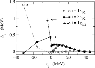
Figure 1: The matrix elements of the pairing potential $\Delta(r)$. These are plotted as a function of the single-particle energy $\epsilon_{j}$ for the state $|\varphi_{j}\rangle$ with a fixed bound state $\langle\varphi_{i}|$, which has the same total and orbital angular momenta $j$ and $l$ as the state $\varphi_{j}$. The open circles, the filled squares, and the open triangles are for the neutron 1$s_{1/2}$ state at $-$31.6 MeV, the 3$s_{1/2}$ state at $-$0.634 MeV, and the 1$g_{9/2}$ state at $-$4.11 MeV, respectively. The diagonal components are denoted by the arrows.

We first discuss the matrix elements $\Delta_{ij}$ of the pairing potential $\Delta(r)$ on the Hartree-Fock basis. Figure 1 shows the matrix elements as a function of the single-particle energy of the state $j$ for a fixed state $i$. For well bound states, such as the 1$s_{1/2}$ state at $\epsilon=-31.6$ MeV, they are all close to zero except for the diagonal component, which is denoted by the arrow (see the open circles). This justifies the success of the BCS approximation for stable nuclei. For weakly bound states, in contrast, the off-diagonal components are the same order as the diagonal component. Specifically, the coupling between the weakly bound state and the positive energy states persist up to about 30 MeV. This is the case both for the $s_{1/2}$ state (the filled square) and for a state with larger angular momentum such as the $g_{9/2}$ state (the open triangle). Since the BCS approximation neglects completely the off-diagonal components of the pairing potential, a careful investigation of the effects of the off-diagonal components is therefore necessary for weakly bound nuclei.

Table 1: The quasi-particle energy $E$ and the occupation probability $v^{2}$ for the four lowest neutron s_1/2 quasi-particle states obtained with several methods. For the BCS method, the corresponding single particle level and the single particle energy are also tabulated.

	$E$ (MeV)	$v^{2}$	s.p. state	$\epsilon$ (MeV)
HFB	0.421	0.553
	1.045	0.039
	2.327	0.010
	4.259	0.003
BCS	0.462	0.645	3s1/2	$-$0.634
	1.010	0.007	4s1/2	$+$0.509
	2.305	0.004	5s1/2	$+$1.803
	4.244	0.002	6s1/2	$+$3.742
p-HFB	0.400	0.606
	1.039	0.033
	2.318	0.005
	4.250	0.001

Let us now solve the HFB equations by diagonalizing the HFB Hamiltonian (4) and compare with the BCS approximation as well as with the p-HFB method discussed in the previous section. We include the single-particle levels up to $\epsilon$= 50 MeV. We have checked that the results do not change significantly even when higher lying states are included. Table 1 compares the HFB method with the BCS approximation for the quasi-particle energy $E$ and the occupation probability $v^{2}$ for the four lowest neutron s_1/2 quasi-particle states. The occupation probability is defined in terms of the quasi-particle wave function as

$$v_{k}^{2}=\int^{\infty}_{0}dr\,|V_{k}(r)|^{2}.$$ (30)

Also shown in the table is the corresponding single-particle state and its energy for the BCS approximation. We find that there is a good correspondence between the HFB and the BCS solutions, especially for the quasi-particle energy. One can thus assign unambiguously a particular single particle state to each HFB state as an unperturbative state.

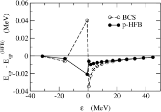
Figure 2: The deviation of the neutron s_1/2 quasi-particle energy, obtained with the BCS method (the dashed line) and the perturbative method p-HFB (the solid line), from the corresponding HFB energy as a function of the single-particle energy.

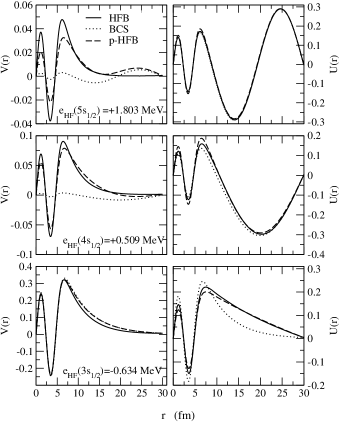
Figure 3: The quasi-particle wave functions for the neutron s_1/2 states obtained with the three methods, HFB, BCS, and p-HFB. The left and the right panels are for the lower ($V$) and the upper ($U$) components of the wave function, respectively. The solid line is the solution of the HFB method, while the dotted line denotes the wave function in the BCS approximation. The result of the perturbative method p-HFB is shown by the dashed line. The top, middle, and bottom panels are for the 5s_1/2, 4s_1/2, and 3s_1/2 states, respectively.

Figure 2 shows the difference in the quasi-particle energy from the HFB energy for the neutron s_1/2 states as a function of the energy of the corresponding single-particle state. The dashed and the solid lines are obtained with the BCS approximation and the perturbation theory, respectively. Surprisingly, the quasi-particle energy is off only by 0.04 MeV at most in the BCS approximation, and the approximation seems to work well as long as the quasi-particle energy is concerned. This is in accordance with the finding in Refs. GSGL01 ; SGL00 ; SGTH03 ; KHL01 . The perturbative method (p-HFB) further improves the result, and the difference in the quasi-particle energy becomes even smaller (see the solid line). Figure 3 compares the quasi-particle wave functions for the first three quasi-particle states. The left and the right panels show the $V(r)$ and the $U(r)$ functions, respectively. The solid, the dotted, and the dashed lines denote the results of the HFB method, the BCS approximation, and the p-HFB method, respectively. As noted by Dobaczewski et al. DNW96 , the smaller component of the wave function in the BCS approximation is inconsistent with the HFB wave function. Notice, however, that the perturbative method p-HFB dramatically improves the radial dependence of the wave function, suggesting that the BCS approximation still provides a good starting point to begin with. For the larger component, although the difference between the HFB and the BCS wave functions is small (but see below for the wave function for the 1g_9/2 state), the perturbation again improves the shape of the wave function in a consistent way. The results of the p-HFB method are summarized in Table 1.

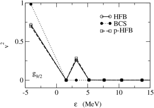
Figure 4: The occupation probability for the $g_{9/2}$ states as a function of the corresponding HF energy $\epsilon$. The solid and the dotted lines are results of the HFB method and the BCS approximation, respectively, while the dashed line is obtained by the perturbative method, p-HFB.

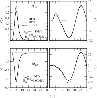
Figure 5: Same as Fig.3, but for the 1$g_{9/2}$ (the upper panel) and the 3$g_{9/2}$ (the lower panel) states.

We next discuss the quasi-particle states which have a relatively large angular momentum. As an example, Fig. 4 compares the occupation probability for the $g_{9/2}$ states obtained by the HFB method (the solid line), the BCS approximation (the dotted line) and the perturbative approach, p-HFB (the dashed line). Again, the p-HFB well reproduces the result of the HFB method. Notice that the occupation probability for the 3$g_{9/2}$ state at the HF energy of $\epsilon=$3.16 MeV is much larger than that in the BCS approximation, which essentially leads to a zero occupation probability for this state. The unperturbed quasi-particle energy, i.e., the quasi-particle energy in the BCS approximation, for this state (3$g_{9/2}$) is 3.66 MeV, which is close to the quasi-particle energy for the 1$g_{9/2}$ state (3.73 MeV). Therefore, according to the perturbation theory, these two states strongly couple to each other by the off-diagonal components of the pairing potential. The wave functions for these two states are plotted in Fig. 5. Indeed, the shape of the wave functions are similar to each other. In the HFB theory, hole states appear as narrow resonance states when the quasi-particle energy is larger than $-\lambda$ DFT84 ; DNW96 ; B00 ; BHR03 ; GSGL01 ; HM03 . The width of the HFB resonance states of this kind originates from the coupling between the hole and the particle states due to the off-diagonal components of the pairing potential. Namely, the particle states which have a similar quasi-particle energy as the hole state in the BCS approximation participate in the resonance state so that the quasi-particle wave functions behave similarly between the hole and the particle states within the resonance widthU67 ; GM70 ; HG04 .

This important mechanism of the particle-hole couplings is missing in the BCS approximation. Note that the 3$g_{9/2}$ state is a non-resonant continuum state in the absence of the pairing. The resonance BCS method, therefore, is not expected to be adequate in the circumstance where details of wave function plays an important role, for instance in the calculation of a strength function with the quasi-particle random phase approximation (QRPA) HS04 ; Y04 .

IV Conclusions

Within the mean-field approach, the pairing correlation is best incorporated with the Hartree-Fock-Bogoliubov (HFB) method. This method consistently takes into account the couplings between the particle-hole and the particle-particle channels, and thus theoretically robust. This method, however, is somewhat cumbersome to solve, and the application of the fully continuum HFB calculation has been limited only to spherical systems so far. The HFB method, being based on the independent quasi-particle approximation, also abandons a simple and intuitive single-particle picture. In this paper, we have developed a perturbative model to the HFB method, which provides an intuitive connection between the HFB and the BCS methods, and at the same time which can be solved much easier than the HFB. Applying the perturbative approach to weakly bound nuclei, we have found that the lowest order perturbation reproduces well the results of the HFB method both for the quasi-particle energy and the radial dependence of wave function. This suggests that the BCS approximation provides good unperturbative states, although it leads to inconsistent quasi-particle wave functions with the HFB wave functions, especially for the smaller component. As good as the self-consistent HFB calculation, one may thus take into account the many-body pairing correlation by using the perturbative model on top of the BCS approximation after the convergence of the BCS calculation is achieved. This scheme might be easily applied to deformed nuclei for which the self-consitent HFB calculation is very dufficult.

We have also pointed out that non-resonant scattering states in a mean-field potential can gain an appreciable occupation probability when there is a weakly bound single particle state close to the Fermi energy. This important coupling effect between particle and hole states cannot be incorporated in the BCS approximation. Evidently, the BCS approximation is inadequate for the QRPA calculations in weakly bound nuclei, where the details of the quasi-particle wave functions play an essential role.

- (1) P. Ring and P. Schuck, The Nuclear Many Body Problem (Springer-Verlag, New York, 1980).
- (2) D.J. Dean and M. Hjorth-Jensen, Rev. Mod. Phys. 75, 607 (2003).
- (3) J. Dobaczewski, H. Flocard, and J. Treiner, Nucl. Phys. A422, 103 (1984).
- (4) J. Dobaczewski, W. Nazarewicz, T.R. Werner, J.F. Berger, C.R. Chinn, and J. Decharge, Phys. Rev. C53, 2809 (1996).
- (5) K. Bennaceur, J. Dobaczewski, and M. Ploszajczak, Phys. Rev. C60, 034308 (1999).
- (6) A. Bulgac, e-print: nucl-th/9907088.
- (7) M. Bender, P.-H. Heenen, and P.-G. Reinhard, Rev. Mod. Phys. 75, 121 (2003).
- (8) M. Grasso, N. Sandulescu, Nguyen Van Giai, and R.J. Liotta, Phys. Rev. C64, 064321 (2001).
- (9) I. Hamamoto and B.R. Mottelson, Phys. Rev. C68,034312 (2003); C69,064302 (2003).
- (10) N. Sandulescu, Nguyen Van Giai, and R.J. Liotta, Phys. Rev. C61, 061301 (R) (2001).
- (11) N. Sandulescu, L.S. Geng, H. Toki, and G.C. Hillhouse, Phys. Rev. C68, 054323 (2003).
- (12) J.R. Bennett, J. Engel, and S. Pittel, Phys. Lett. B368, 7 (1996).
- (13) A.T. Kruppa, P.H. Heenen, and R.J. Liotta, Phys. Rev. C63, 044324 (2001).
- (14) B. Gall, P. Bonche, J. Dobaczewski, H. Flocard, and P.-H. Heenen, Z. Phys. A348, 183 (1994).
- (15) J. Terasaki, P.-H. Heenen, P. Bonche, J. Dobaczewski, and H. Flocard, Nucl. Phys. A593, 1 (1995).
- (16) J. Terasaki, P.-H. Heenen, H. Flocard, and P. Bonche, Nucl. Phys. A600, 371 (1996).
- (17) J. Terasaki, H. Flocard, P.-H. Heenen, and P. Bonche, Nucl. Phys. A621, 706 (1997).
- (18) H.-J. Unger, Nucl. Phys. A104, 564 (1967).
- (19) Nguyen Van Giai and C. Marty, Nucl. Phys. A150, 593 (1970).
- (20) K. Hagino and Nguyen Van Giai, Nucl. Phys. A735, 55 (2004).
- (21) I. Hamamoto and H. Sagawa, Phys. Rev. C70, 034317 (2004).
- (22) M. Yamagami, e-print:nucl-th/0404030.