Phase structure of the two-fluid proton-neutron system

Abstract

The phase structure of a two-fluid bosonic system is investigated. The proton-neutron interacting boson model (IBM-2) posesses a rich phase structure involving three control parameters and multiple order parameters. The surfaces of quantum phase transition between spherical, axially-symmetric deformed, and $\mathrm{SU}_{\pi\nu}^{*}(3)$ triaxial phases are determined.

The phase structure of quantum many-body systems has in recent years been a subject of great experimental and theoretical interest. Models based upon algebraic Hamiltonians have found extensive application to the spectroscopy of many-body systems, including nuclei iachello1987:ibm and molecules iachello1995:vibron . Applications to hadrons have also been developed bijker1994:algebraic-hadron-nonstrange . For certain specific forms of its Hamiltonian, an algebraic model exhibits dynamical symmetries. In the classical limit, these dynamical symmetries correspond to qualitatively distinct ground-state equilibrium configurations, which constitute the phases of the system gilmore1978:coherent ; feng1981:ibm-phase . The phase structure has been studied in detail for algebraic models describing systems composed of one species of constituent particle (“one-fluid” systems), in particular the interacting boson model (IBM) iachello1987:ibm for nuclei. While one-fluid systems are described by a single elementary Lie algebra, usually $\mathrm{U}(n)$, multi-fluid systems are described by a coupling of such Lie algebras, $\mathrm{U}_{1}(n)\otimes\mathrm{U}_{2}(n)\otimes\cdots$ iachello1987:ibm ; iachello1995:vibron . This more involved algebraic structure naturally leads to a richer phase structure.

In the present work, the phase structure of a system comprised of two interacting fluids is investigated. The proton-neutron interacting boson model (IBM-2) arima1977:ibm2-shell ; iachello1987:ibm , in which proton pairs and neutron pairs are treated as distinct constituents, is considered. While the one-fluid IBM exhibits three dynamical symmetries, separated by first and second order phase transitions dieperink1980:ibm-classical ; feng1981:ibm-phase , the IBM-2 supports four dynamical symmetries vanisacker1986:ibm2-limits ; dieperink1982:ibm2-triax , and thus inherently has a higher-dimensional phase diagram. Moreover, the phase structure is found to posess qualitatively new features. Due to the complexity of the problem, a combination of analytic and numerical methods have been applied in this analysis. Preliminary investigations of the IBM-2 phase structure have been presented in Refs. arias2004:ibmpn-icnpls04 ; caprio2004:ibmpn-icnpls04 .

Before proceeding, let us briefly summarize the IBM-2 Hamiltonian and the dynamical symmetries it supports. Operators in the IBM-2 are constructed from the generators of the group $\mathrm{U}_{\pi}(6)\otimes\mathrm{U}_{\nu}(6)$, realized in terms of the boson creation operators $s_{\rho,0}^{{\dagger}}$ and $d_{\rho,\mu}^{{\dagger}}$ (where $\rho$ represents $\pi$ or $\nu$, and $\mu$$=$$-2,\ldots,2$) and their associated annihilation operators, acting on a basis of good boson numbers $N_{\pi}$ and $N_{\nu}$. A schematic Hamiltonian which retains the essential features of the model is the $F$-spin invariant Hamiltonian (e.g., Ref. lipas1990:ibm2-fspin )

$$H=\varepsilon(\hat{n}_{d\pi}+\hat{n}_{d\nu})+\kappa(\hat{Q}_{\pi}^{\chi_{\pi}}+\hat{Q}_{\nu}^{\chi_{\nu}})\cdot(\hat{Q}_{\pi}^{\chi_{\pi}}+\hat{Q}_{\nu}^{\chi_{\nu}}),$$ (1)

where $\hat{n}_{d\rho}\equiv d_{\rho}^{{\dagger}}\cdot\tilde{d}_{\rho}$ and $\hat{Q}_{\rho}^{\chi_{\rho}}\equiv(s_{\rho}^{{\dagger}}\times\tilde{d}_{\rho}+d_{\rho}^{{\dagger}}\times\tilde{s}_{\rho})^{(2)}+\chi_{\rho}(d_{\rho}^{{\dagger}}\times\tilde{d}_{\rho})^{(2)}$. It is convenient to also introduce “scalar” and “vector” parameters $\chi_{S}$$\equiv$$\frac{1}{2}(\chi_{\pi}+\chi_{\nu})$ and $\chi_{V}$$\equiv$$\frac{1}{2}(\chi_{\pi}-\chi_{\nu})$. Three of the IBM-2 symmetries occur for $\chi_{V}$$=$$0$ and have direct analogues in the one-fluid IBM vanisacker1986:ibm2-limits : $\mathrm{U}_{\pi\nu}(5)$ ($\kappa=0$), for which the geometric interpretation is that of undeformed proton and neutron fluids, $\mathrm{SO}_{\pi\nu}(6)$ ($\varepsilon=0$, $\chi_{\pi}=\chi_{\nu}=0$), yielding deformed, $\gamma$-unstable structure, and $\mathrm{SU}_{\pi\nu}(3)$ ($\varepsilon=0$, $\chi_{\pi}=\chi_{\nu}=-\sqrt{7}/2$), for which prolate axially symmetric structure is obtained. [The complementary case $\chi_{\pi}$$=$$\chi_{\nu}$$=$$+\sqrt{7}/2$, giving oblate axially symmetric structure, is distinguished by the notation $\overline{\mathrm{SU}_{\pi\nu}(3)}$.] However, a symmetry special to the IBM-2, denoted $\mathrm{SU}_{\pi\nu}^{*}(3)$, is obtained for $\varepsilon=0$, $\chi_{\pi}=-\sqrt{7}/2$, and $\chi_{\nu}=+\sqrt{7}/2$ dieperink1982:ibm2-triax . The equilibrium configuration consists of a proton fluid with axially symmetric prolate deformation coupled to a neutron fluid with axially symmetric oblate deformation, with their symmetry axes orthogonal to each other dieperink1982:ibm2-triax ; leviatan1990:ibm2-modes ; ginocchio1992:ibm2-shapes , yielding an overall composite nuclear shape with triaxial deformation. To avoid ambiguity, we shall adopt here the notation $\overline{\mathrm{SU}_{\pi\nu}^{*}(3)}$ for the complementary case $\chi_{\pi}=+\sqrt{7}/2$ and $\chi_{\nu}=-\sqrt{7}/2$, for which the proton and neutron deformations are interchanged.

The classical limit of the IBM-2 is obtained by evaluation of the expectation value of $H$ for the coherent state $|N_{\pi},\alpha^{(2)}_{\pi};N_{\nu},\alpha^{(2)}_{\nu}\rangle$$\propto$ $(s_{\pi,0}^{\dagger}+\sum_{\mu}\alpha^{(2)}_{\pi,\mu}d_{\pi,\mu}^{\dagger})^{N_{\pi}}(s_{\nu,0}^{\dagger}+\sum_{\mu}\alpha^{(2)}_{\nu,\mu}d_{\nu,\mu}^{\dagger})^{N_{\nu}}|0\rangle$. This yields an energy surface $\mathcal{E}$$\equiv$$\langle H\rangle$ as a function of the coherent state parameters $\alpha^{(2)}_{\rho,\mu}$. The $\alpha^{(2)}_{\rho,\mu}$ are interpreted geometrically as the quadrupole shape variables bohr1998:v2 for the proton and neutron fluids and are equivalent to four deformation parameters ($\beta_{\pi}$, $\gamma_{\pi}$, $\beta_{\nu}$, and $\gamma_{\nu}$) and six Euler angles ($\theta_{1\pi}$, $\theta_{2\pi}$, $\theta_{3\pi}$, $\theta_{1\nu}$, $\theta_{2\nu}$, and $\theta_{3\nu}$). By rotational invariance, $\mathcal{E}$ depends only upon the relative Euler angles $\vartheta_{i}$ between the proton and neutron fluid intrinsic systems, not the $\theta_{i\pi}$ and $\theta_{i\nu}$ separately. Minimization of $\mathcal{E}(\beta_{\pi},\gamma_{\pi},\beta_{\nu},\gamma_{\nu},\vartheta_{1},\vartheta_{2},\vartheta_{3})$ with respect to its parameters yields the classical equilibrium configuration of the ground state. The terms $\langle\hat{n}_{d\pi}\rangle$, $\langle\hat{n}_{d\nu}\rangle$, $\langle\hat{Q}_{\pi}\cdot\hat{Q}_{\pi}\rangle$, and $\langle\hat{Q}_{\nu}\cdot\hat{Q}_{\nu}\rangle$ contributing to $\mathcal{E}$ involve only a single fluid and are thus known from the IBM (see Ref. vanisacker1981:ibm-triax ). The expectation value $\langle\hat{Q}_{\pi}\cdot\hat{Q}_{\nu}\rangle$ of the interaction term is obtained by the methods of Refs. vanisacker1981:ibm-triax ; ginocchio1992:ibm2-shapes as a function of all seven possible parameters ($\beta_{\pi}$, $\gamma_{\pi}$, $\beta_{\nu}$, $\gamma_{\nu}$, $\vartheta_{1}$, $\vartheta_{2}$, and $\vartheta_{3}$),

$$\langle\hat{Q}_{\pi}^{\chi_{\pi}}\cdot\hat{Q}_{\nu}^{\chi_{\nu}}\rangle=\frac{N_{\pi}N_{\nu}}{(1+\beta_{\pi}^{2})(1+\beta_{\nu}^{2})}[\alpha_{\pi}^{(2)\,*}+\tilde{\alpha}_{\pi}^{(2)}+\chi_{\pi}(\alpha_{\pi}^{(2)\,*}\times\tilde{\alpha}_{\pi}^{(2)})^{(2)}]\\ \cdot[\alpha_{\nu}^{(2)\,*}+\tilde{\alpha}_{\nu}^{(2)}+\chi_{\nu}(\alpha_{\nu}^{(2)\,*}\times\tilde{\alpha}_{\nu}^{(2)})^{(2)}],$$ (2)

where

$$\alpha_{\rho,\mu}^{(2)}=\beta_{\rho}\cos\gamma_{\rho}D^{2\,*}_{\mu 0}(\theta_{1\rho},\theta_{2\rho},\theta_{3\rho})\\ +\frac{1}{\sqrt{2}}\beta_{\rho}\sin\gamma_{\rho}\bigl{[}D^{2\,*}_{\mu 2}(\theta_{1\rho},\theta_{2\rho},\theta_{3\rho})+D^{2\,*}_{\mu-2}(\theta_{1\rho},\theta_{2\rho},\theta_{3\rho})\bigr{]}$$ (3)

and where the Euler angles may be chosen to be $\theta_{i\pi}=0$ and $\theta_{i\nu}=\vartheta_{i}$ by rotational invariance. The $\langle\hat{n}_{d\rho}\rangle$ are linear in $N_{\pi}$ or $N_{\nu}$, while the $\langle\hat{Q}_{\rho}\cdot\hat{Q}_{\rho^{\prime}}\rangle$ are quadratic. It is thus convenient to reparametrize the Hamiltonian (1) as

$$H=\frac{1-\xi^{\prime}}{N}(\hat{n}_{d\pi}+\hat{n}_{d\nu})-\frac{\xi^{\prime}}{N^{2}}(\hat{Q}_{\pi}^{\chi_{\pi}}+\hat{Q}_{\nu}^{\chi_{\nu}})\cdot(\hat{Q}_{\pi}^{\chi_{\pi}}+\hat{Q}_{\nu}^{\chi_{\nu}}),$$ (4)

where $N\equiv N_{\pi}+N_{\nu}$, so that the energy function $\mathcal{E}$ is independent of $N$ at fixed ratio $N_{\pi}/N_{\nu}$. This definition also condenses the full range of possible ratios $\varepsilon/\kappa$ onto the finite interval $0\leq\xi^{\prime}\leq 1$. An overall normalization parameter for $H$ has been discarded as irrelevant to the structure of the energy surface. There are thus three control parameters — $\xi^{\prime}$, $\chi_{\pi}$, and $\chi_{\nu}$ — for this Hamiltonian.

A simple categorization of the possible Euler angle and $\gamma_{\rho}$ values for the equilibrium configurations for certain IBM-2 energy surfaces has been presented in Ref. ginocchio1992:ibm2-shapes . For a class of Hamiltonians including the present one (4), it is found that the global minimum only occurs for vanishing relative Euler angles, i.e., for aligned proton and neutron intrinsic frames. This effectively reduces the number of order parameters for the system from seven to four — $\beta_{\pi}$, $\gamma_{\pi}$, $\beta_{\nu}$, and $\gamma_{\nu}$.

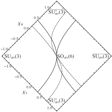
Figure 1: Phase diagram for the $\mathrm{SU}_{\pi\nu}(3)$-$\mathrm{SO}_{\pi\nu}(6)$-$\mathrm{SU}_{\pi\nu}^{*}(3)$ plane ($\xi^{\prime}=1$) in the parameter space of the Hamiltonian of (4), showing the second-order phase transition curves (6) for the cases $N_{\pi}/N_{\nu}=1$ (solid) and $N_{\pi}/N_{\nu}=4$ (dashed). The diagram is rotated to allow more direct comparison with Fig. 2.

The orders of phase transitions are, in the present study, determined according to the Ehrenfest classification: a phase transition is first order if the first derivative of the system’s energy is discontinuous with respect to the control parameter being varied, second order if the second derivative is discontinuous, etc. Where the system’s energy is obtained, as in the present classical analysis, as the global minimum of an energy function $\mathcal{E}$, a first order transition is usually associated with a discontinuous jump in the equilibrium coordinates (“order parameters”) between distinct competing minima. Second or higher order transitions are associated instead with a continuous evolution of the equilibrium coordinates, as when an initially solitary global minimum becomes unstable (posessing a vanishing second derivative with respect to some coordinate) and evolves into two or more minima. It should be noted that, whenever the order of a phase transition is obtained by numerical analysis, application of the Ehrenfest criterion is limited by the ability to numerically resolve sufficiently small discontinuities, especially a consideration for points of first-order transition very close to a point of second-order transition. Moreover, problems with the classification scheme, not addressed here, may arise at the boundaries of the parameter space or when the Hamiltonian posesses additional symmetries.

We begin our analysis with an analytic study of the phase structure of the Hamiltonian (4) for $\xi^{\prime}=1$, which encompasses the $\mathrm{SO}_{\pi\nu}(6)$, $\mathrm{SU}_{\pi\nu}(3)$, and $\mathrm{SU}_{\pi\nu}^{*}(3)$ dynamical symmetries (see Fig. 1). The global equilibrium in this case is always deformed ($\beta_{\pi}>0$ and $\beta_{\nu}>0$). Surrounding the $\mathrm{SU}_{\pi\nu}(3)$ dynamical symmetry is a region of parameter space in which the equilibrium deformations are axially symmetric ($\gamma_{\pi}=\gamma_{\nu}=0^{\circ}$), and a similar region surrounds the $\overline{\mathrm{SU}_{\pi\nu}(3)}$ dynamical symmetry ($\gamma_{\pi}=\gamma_{\nu}=60^{\circ}$). Taking the $\mathrm{SU}_{\pi\nu}(3)$-like region for specificity, the global minimum occurs for

$$\beta_{\rho}=\Biggl{[}\Biggl{(}\frac{\chi_{\rho}}{\sqrt{14}}\Biggr{)}^{2}+1\Biggr{]}^{1/2}-\frac{\chi_{\rho}}{\sqrt{14}}.$$ (5)

At the boundary of this region, axial equilibrium deformation gives way to triaxial deformation, with $\gamma_{\pi}$ and/or $\gamma_{\nu}$ nonzero. This transition occurs continuously on the locus of points at which the minimum given by (5) first becomes unstable with respect to $\gamma$ deformation. Since $\mathcal{E}$ depends upon both $\gamma_{\pi}$ and $\gamma_{\nu}$, instablility occurs when the directional second derivative of $\mathcal{E}$ first vanishes along some “direction” in $(\gamma_{\pi},\gamma_{\nu})$ coordinate space, which may generally happen before either $\partial^{2}\mathcal{E}/\partial\gamma_{\pi}^{2}$ or $\partial^{2}\mathcal{E}/\partial\gamma_{\nu}^{2}$ vanishes individually. The equation describing the boundary curve in $\chi_{\pi}$ and $\chi_{\nu}$ is most compactly expressed in terms of the corresponding equilibrium values $\beta_{\pi}$ and $\beta_{\nu}$ from (5) as

$$1=\frac{9\frac{N_{\pi}}{N_{\nu}}\beta_{\pi}(\beta_{\pi}^{2}-1)+\beta_{\nu}(2\beta_{\pi}^{2}-1)(\beta_{\pi}^{2}+1)}{2\beta_{\pi}(\beta_{\pi}^{2}-2)^{2}}\\ \times\frac{9\frac{N_{\nu}}{N_{\pi}}\beta_{\nu}(\beta_{\nu}^{2}-1)+\beta_{\pi}(2\beta_{\nu}^{2}-1)(\beta_{\nu}^{2}+1)}{2\beta_{\nu}(\beta_{\nu}^{2}-2)^{2}}.$$ (6)

This curve is shown in Fig. 1. Along the $\mathrm{SU}_{\pi\nu}(3)$-$\mathrm{SU}_{\pi\nu}^{*}(3)$ line ($\chi_{\pi}=-\sqrt{7}/2$), for $N_{\pi}/N_{\nu}=1$ the transition occurs at $\chi_{\nu}\approx 0.4035$, at which point the global minimum becomes soft with respect to $\gamma_{\nu}$ at fixed $\gamma_{\pi}=0^{\circ}$.

Returning to the full parameter space for the three-parameter Hamiltonian of (4), limited but useful analytic results can also be obtained for the transition between undeformed ($\beta_{\pi}=\beta_{\nu}=0$) and deformed structure. The parameter space is illustrated in Fig. 2.

For $\chi_{V}$$=$$0$, i.e., in the “base” plane in Fig. 2, the analysis is closely related to that for the one-fluid IBM. The equilibrium configurations all have $\beta_{\pi}=\beta_{\nu}(\equiv\beta)$ and are identical to those obtained for the IBM Hamiltonian $H_{\text{IBM}}=[(1-\xi^{\prime})/N]\hat{n}_{d}-(\xi^{\prime}/N^{2})\hat{Q}^{\chi}\cdot\hat{Q}^{\chi}$ with $\chi=\chi_{S}$, the phase structure of which is well known dieperink1980:ibm-classical ; feng1981:ibm-phase . A second-order transition between undeformed ($\beta=0$) and deformed ($\beta\neq 0$) structure occurs at the parameter values $\xi^{\prime}=1/5$ and $\chi=0$, for which the minimum in the energy surface at $\beta=0$ is unstable. This point lies on a trajectory of first-order transition points, at which a distinct minimum with nonzero $\beta$ preempts that with $\beta=0$ as global minimum.

Figure 2: Phase diagram of the proton-neutron interacting boson model (IBM-2) for the Hamiltonian of (4), as obtained by numerical minimization of $\mathcal{E}$, for $N_{\pi}/N_{\nu}=1$. The surfaces of first-order (red) and second-order (blue) transition between regions of undeformed, axially symmetric deformed, and triaxially deformed equilibria are shown. Only one “quadrant” of parameter space ($0\leq\xi^{\prime}\leq 1$, $-\sqrt{7}/2\leq\chi_{S}\leq 0$, and $0\leq\chi_{V}\leq\sqrt{7}/2$) is included in this plot, since the others may be obtained by reflection. The $\chi_{S}$ and $\chi_{V}$ axes are scaled by $\xi^{\prime}$, so as to converge to a point at the $\mathrm{U}_{\pi\nu}(5)$ limit.

A second-order transition from undeformed to deformed structure occurs when the minimum of $\mathcal{E}$ at $\beta_{\pi}=\beta_{\nu}=0$ becomes unstable with respect to $\beta$ deformation, provided this minimum is the global minimum (that is, provided it has not been rendered irrelevant by a prior first-order transition to another, deformed minimum). The derivative indicating such $\beta$ softness is the directional second derivative $\partial^{2}\mathcal{E}/\partial\beta^{2}$ along a ray $\beta_{\pi}=u_{\pi}\beta$ and $\beta_{\nu}=u_{\nu}\beta$ (i.e., fixed $\beta_{\pi}/\beta_{\nu}$) at fixed $\gamma_{\pi}$ and $\gamma_{\nu}$, evaluated at $\beta=0$. This quantity is independent of $\chi_{S}$ and $\chi_{V}$ [e.g., for $N_{\pi}/N_{\nu}=1$, $\partial^{2}\mathcal{E}/\partial\beta^{2}|_{\beta=0}=(1-3\xi^{\prime})(u_{\pi}^{2}+u_{\nu}^{2})-4\xi^{\prime}u_{\pi}u_{\nu}\cos(\gamma_{\pi}-\gamma_{\nu})$]. The minimum at zero deformation first becomes unstable at $\xi^{\prime}=1/5$, where it is soft against deformations with $\beta_{\pi}=\beta_{\nu}$ and $\gamma_{\pi}=\gamma_{\nu}(\equiv\gamma)$, for any value of $\gamma$.

The curve of first-order phase transition in the plane $\chi_{V}=0$ arises from competition between the undeformed minimum and one with $\beta_{\pi}=\beta_{\nu}\neq 0$ and $\gamma_{\pi}=\gamma_{\nu}=0^{\circ}$. The special “slice” $\mathcal{E}(\beta_{\pi}=\beta,\beta_{\nu}=\beta,\gamma_{\pi}=0,\gamma_{\nu}=0)$ of the energy function, which includes both these minima, is found for $N_{\pi}/N_{\nu}=1$ to be independent of $\chi_{V}$ at fixed $\xi^{\prime}$ and $\chi_{S}$, i.e., invariant along any vertical line in Fig. 2. Thus, the first-order phase transitions occuring in the plane $\chi_{V}=0$ at $\xi^{\prime}<1/5$ “propagate” out of this plane. [To the approximation that $\beta_{\pi}\approx\beta_{\nu}$ for the deformed minimum, the first-order transition surface for $\chi_{V}\neq 0$ is obtained by vertical extension of the one-fluid IBM transition trajectory in Fig. 2.] The occurence of a second-order phase transition at $\xi^{\prime}=1/5$ is thus precluded everywhere except along a vertical line in parameter space extending through the one-fluid IBM second-order transition point. It is verified numerically, as described below, that the undeformed minimum is indeed global along this line. The line $\xi^{\prime}=1/5$ and $\chi_{S}=0$ is thus a locus of second-order transition between zero and nonzero deformation. These results are readily generalized to arbitrary $N_{\pi}/N_{\nu}$, for which the invariance of $\mathcal{E}$ occurs along lines of constant $N_{\pi}\chi_{\pi}+N_{\nu}\chi_{\nu}$ and the line of second-order phase transition obeys $\chi_{\pi}/\chi_{\nu}=-N_{\nu}/N_{\pi}$.

The remainder of the phase diagram is obtained by numerical minimization of the energy surface with respect to $\beta_{\pi}$, $\gamma_{\pi}$, $\beta_{\nu}$, and $\gamma_{\nu}$. For robust identification of the global minimum, $\mathcal{E}$ is first evaluated at each point on a fine mesh in these coordinates ($\Delta\beta_{\rho}=0.03$, $\Delta\gamma_{\rho}=2^{\circ}$), and all points which are discrete local minima of $\mathcal{E}$ relative to the neighboring mesh points are identified. The $\beta_{\pi}$, $\gamma_{\pi}$, $\beta_{\nu}$, and $\gamma_{\nu}$ values for these minima are then refined by an iterative method. The global minimum is identified from among these.

The phase diagram obtained in this fashion is shown in Fig. 2 for the case $N_{\pi}/N_{\nu}=1$. Numerical investigation of the behavior of $\mathcal{E}$ at the transition points allows the Ehrenfest criterion to be applied, and it appears that the axial-triaxial transition is everywhere second order.

The IBM-2 phase diagram obtained here provides a framework for studying the transition between axial and triaxial structure in nuclei. Triaxial nuclear deformation might arise from several different sources: higher-order (cubic, quartic, etc.) interactions in an essentially one-fluid nucleus vanisacker1981:ibm-triax , distinct deformations of the proton and neutron fluids as discussed here, or the presence of configurations involving hexadecapole nucleon pairs heyde1983:ibm-g-boson-104ru . The present analysis provides insight into the conditions under which proton-neutron triaxial deformation may occur and the nature of the transition to such structure. Phenomenological studies extending this work should make use of a more realistic Hamiltonian involving a Majorana contribution and different strengths for the $\hat{Q}_{\rho}\cdot\hat{Q}_{\rho^{\prime}}$ terms (e.g., Ref. lipas1990:ibm2-fspin ). Such studies will provide guidance for the experimental investigation of triaxial structure as progressively more neutron rich nuclei become accessible.

The present analysis may serve as a model for the study of other multi-fluid bosonic systems. Within nuclear physics, the $\mathrm{U}_{\text{core}}(6)\otimes\mathrm{U}_{\text{skin}}(6)$ description of core-skin collective modes in neutron rich nuclei warner1997:skin-soft-scissors can be treated similarly. In molecular physics, a study of the phase structure is in progress for the vibron model with two vibronic species iachello1995:vibron , where it is relevant to coupled vibronic bending modes in acetylene. Another area of potential application of the method is to atomic Bose-Einstein condensates. Scissors modes, introduced originally within the framework of nuclear two-rotor models loiudice1978:scissors and the IBM-2 iachello-scissors-COMBO , have been observed for oscillations of a single-constituent Bose-Einstein condensate relative to an anisotropic potential marago2000:bec-scissors . Experiments are planned to produce condensates of two different atomic species and to study the scissors modes between them. Triaxial deformations of the type considered here could then occur, and a directly analogous analysis could be applied.

The exotic features of the phase diagram considered here, arising from the presence of multiple control parameters and multiple order parameters, are likely to be encountered for other multi-fluid systems as well. They will require a classification scheme beyond the simple Ehrenfest or one-parameter Landau models for their proper description.

- (1) F. Iachello and A. Arima, The Interacting Boson Model (Cambridge University Press, Cambridge, 1987).
- (2) F. Iachello and R. D. Levine, Algebraic Theory of Molecules (Oxford University Press, Oxford, 1995).
- (3) R. Bijker, F. Iachello, and A. Leviatan, Ann. Phys. (N.Y.) 236, 69 (1994).
- (4) R. Gilmore, J. Math. Phys. 20, 891 (1979).
- (5) D. H. Feng, R. Gilmore, and S. R. Deans, Phys. Rev. C 23, 1254 (1981).
- (6) A. Arima, T. Otsuka, F. Iachello, and I. Talmi, Phys. Lett. B 66, 205 (1977).
- (7) A. E. L. Dieperink, O. Scholten, and F. Iachello, Phys. Rev. Lett. 44, 1747 (1980).
- (8) P. Van Isacker, K. Heyde, J. Jolie, and A. Sevrin, Ann. Phys. (N.Y.) 171, 253 (1986).
- (9) A. E. L. Dieperink and R. Bijker, Phys. Lett. B 116, 77 (1982).
- (10) R. Bijker, R. F. Casten, and A. Frank, eds., Nuclear Physics, Large and Small: International Conference on Microscopic Studies of Collective Phenomena, AIP Conf. Proc. 726 (AIP, Melville, NY, 2004).
- (11) J. M. Arias, J. Dukelsky, and J. E. García-Ramos, in Ref. proc-icnpls04 , p. 127.
- (12) M. A. Caprio, in Ref. proc-icnpls04 , p. 215.
- (13) P. O. Lipas, P. von Brentano, and A. Gelberg, Rep. Prog. Phys. 53, 1355 (1990).
- (14) A. Leviatan and M. W. Kirson, Ann. Phys. (N.Y.) 201, 13 (1990).
- (15) J. N. Ginocchio and A. Leviatan, Ann. Phys. (N.Y.) 216, 152 (1992).
- (16) A. Bohr and B. R. Mottelson, Nuclear Deformations, Vol. 2 of Nuclear Structure (World Scientific, Singapore, 1998).
- (17) P. Van Isacker and Jin-Quan Chen, Phys. Rev. C 24, 684 (1981).
- (18) K. Heyde, P. van Isacker, M. Waroquier, G. Wenes, Y. Gigase, and J. Stachel, Nucl. Phys. A 398, 235 (1983).
- (19) D. D. Warner and P. Van Isacker, Phys. Lett. B 395, 145 (1997).
- (20) N. Lo Iudice and F. Palumbo, Phys. Rev. Lett. 41, 1532 (1978).
- (21) F. Iachello, Nucl. Phys. A 358, 89c (1981); Phys. Rev. Lett. 53, 1427 (1984).
- (22) O. M. Maragò, S. A. Hopkins, J. Arlt, E. Hodby, G. Hechenblaikner, and C. J. Foot, Phys. Rev. Lett. 84, 2056 (2000).