Leading-order Corrections of a Dynamical Model for Electromagnetic Pion Production Reactions

Abstract

By applying a unitary transformation method, we have derived the leading-order corrections on the effective Hamiltonian of a dynamical model developed in Phys. Rev. C54, 2660 (1996) for electromagnetic pion production reactions. The resulting $energy$-$independent$ one-loop corrections on the baryon masses and the $\gamma N\rightarrow\Delta$ vertex interaction are associated with the structure of the nucleon and $\Delta$ and have been calculated within a constituent quark model. We find that the one-loop corrections on the magnetic M1 transition of the $\gamma N\rightarrow\Delta$ are very small, while their contributions to the electric E2 and Coulomb C2 transitions are found to be in opposite signs of that due to pion cloud effects associated with the scattering states. Our results further indicate that the determination of the nonspherical $L=2$ components of the constituent quark wavefunctions of $N$ and $\Delta$ from the extracted empirical E2 and C2 form factors requires a rigorous and complete calculation of meson cloud effects. We also find that the one-loop corrections on the non-resonant pion production operator can resolve the difficulty in describing the near threshold $\gamma p\rightarrow\pi^{0}p$ reaction. Possible future developments are discussed.

I Introduction

In the past few years, extensive and precise data of electromagnetic meson production reactions have become available and some of these data have been used to extract the information about the nucleon resonancesburkert . On the other hand, theoretical models for analyzing these reactions are still far from complete. Even in the simplest and well-studied $\Delta$ excitation region, none of the most often applied modelssl1 ; sl2 ; kamyan ; dmt ; maid has been able to give $predictions$ which agree perfectly with the single pion production data accumulated recently, in particular the data on spin observables and longitudinal-transverse interference cross sections. While these models can give an overall good description of fairly extensive data, efforts must be made to remove the remaining discrepancies such that a complete understanding of the $\Delta$ resonance can be obtained. The experiences gained from these efforts will undoubtly be very useful for investigating the much more complex higher mass $N^{*}$ resonances. In this work, we report on the progress we have made in this direction, focusing on the dynamical model we have developed in Refs.sl1 ; sl2 (called the Sato-Lee (SL) model in the literatures). In particular, we would like to explore how the bare $\gamma N\rightarrow\Delta$ parameters extracted within the SL model can be better understood in terms of the structure of $N$ and $\Delta$. We would also like to see how the non-resonant pion production operator in the SL model can be improved.

We first recall one of the most interesting results from the SL model. It was found that the pion cloud effects give very large contributions to the $\gamma N\rightarrow\Delta$ transition form factors and is the source of the differences between the values predicted by the conventional constituent quark model and that extracted from empirical amplitude analyses. The predicted very pronounced $Q^{2}-$dependence in electric $E2$ and Coulomb $C2$ transitions have motivated several recent experimental efforts. These pion cloud effects are calculated from the following expression

$$\bar{\Gamma}_{\gamma N,\Delta}(W,q)=\Gamma^{0}_{\gamma N,\Delta}(q)+\int dkk^{2}v^{tree}_{\gamma\pi}(q,k)\frac{1}{W-E_{\pi}(k)-E_{N}(k)+i\epsilon}\bar{\Gamma}_{\pi N,\Delta}(W,k)$$

where $\Gamma^{0}_{\gamma N,\Delta}$ is the bare vertex, $v^{tree}_{\gamma,\pi}$ is the non-resonant $\gamma N\rightarrow\pi N$ amplitude calculated from the standard Pseudo-Vector Born terms and the $\rho$ and $\omega$ exchanges, and $\bar{\Gamma}_{\pi N,\Delta}(W,k)$ is the dressed $\Delta\rightarrow\pi N$ vertex. One observes from the above equation that these pion cloud effects are due to pions in the $scattering$ states which can reach the on-shell momentum asymptotically.

We now examine how the above procedure is related to our current understanding of hadron structure. Because of the chiral symmetry of QCD is spontaneously broken, it is generally believed that in the region where the momentum transfer is not too large the structure of the nucleon and $\Delta$ can be considered as systems made of constituent quarks and virtual pions. We thus expect that their responses to the external electromagnetic field can be from the constituent quarks and also from the virtual pions. Obviously the pion-loop integration in the above equation do not account for all of the effects due to the virtual pions in hadrons. The leading term $\Gamma^{0}_{\gamma N,\Delta}$ must still contain some effects due to virtual pions which never go on-shell during the $N$-$\Delta$ transitions. In this work, we will show how the corrections due to these virtual pion cloud effects can be derived by applying the unitary transformation method. In a consistent derivation, the one-loop corrections on the non-resonant pion production operator of the SL model have also been derived. These one-loop corrections are also energy-independent and are different from those due to pions in $scattering$ states. These corrections are expected to have important effects in the region where the pion electromagnetic reactions are sensitive to the non-resonant amplitudes.

In section II, we recall a dynamical formulation within which the leading order one-loop corrections on the effective Hamiltonian of the SL model are derived. In section III, the consequences of these leading order corrections on the $\gamma N\rightarrow\Delta$ transitions are calculated and interpreted within a constituent quark model. The one-loop corrections on the non-resonant pion production operator are then investigated in section IV, focusing on the s-wave amplitude of the near threshold $\pi^{0}$ photoproduction reaction. Possible future developments are discussed in section V.

II Formulation

As explained in Ref.sl1 , the SL model is constructed by applying a unitary transformation method to deduce from relativistic quantum field theory an effective Hamiltonian for describing meson-baryon reactions. The details of the employed unitary transformation has been given in Refs.sl1 ; ksh and will not be repeated in this paper. Here we only emphasize that the starting point of the unitary transformation method is a field theoretical Lagrangian density. This is identical to other more familiar approaches for constructing dynamical models of meson-baryon interactions, such as those based on the ladder Bethe-Salpetertjon ; afnan or three-dimensional ladder Bethe-Salpeter equationspearce ; gross ; hung ; julich ; pasca . In the lowest order, all approaches yield very similar, if not completely identical, scattering amplitudes. Their differences are in the resulting dynamical equations which are used to include nonperturbatively certain classes of higher order effects that are deemed to be important for the processes considered.

To illustrate the unitary transformation method, it is sufficient to consider a model Lagrangian density $L(\psi_{N},\psi_{\Delta},\phi_{\pi})$ describing the pseudo-vector coupling between $\pi$, $N$ and $\Delta$ fields. By using the standard canonical quantization procedure, a Hamiltonian can be constructed. To simplify the presentation, the spin and isospin variables as well as the anti-particle components are suppressed here. The resulting Hamiltonian can then be schematically written as

$$H=H_{0}+H_{I}+H_{em}\,,$$ (1)

with

$$H_{0}=\sum_{B}\int d\bm{p}b^{\dagger}_{B}(\bm{p})b_{B}(\bm{p})E_{B}(\bm{p})+\int d\bm{k}a^{\dagger}_{\pi}(\bm{k})a_{\pi}(\bm{k})E_{\pi}(\bm{k})$$

where $b^{\dagger}_{B}(\bm{p})(b_{B}(\bm{p}))$ is the creation(annihilation) operator for a baryon with momentum $\bm{p}$, and $a^{\dagger}(\bm{k})(a(\bm{k}))$ for a pion with momentum $\bm{k}$. The energy is defined as $E_{\alpha}(\bm{p})=(m_{\alpha}+\bm{p}^{2})^{1/2}$ with $m_{\alpha}$ denoting the mass of particle $\alpha$. Clearly, $H_{0}$ is the sum of free energy operators for baryons($B=N,\Delta$) and pion($\pi)$. The strong interaction Hamiltonian in Eq. (1) is

$$H_{I}=\sum_{B,B^{\prime}}[\Gamma^{0}_{\pi B^{\prime},B}+\mbox{h.c.}]\,,$$ (2)

with

$$\Gamma^{0}_{\pi B^{\prime},B}=\int d\bm{p}d\bm{k}b^{\dagger}_{B^{\prime}}(\bm{p}-\bm{k})b_{B}(\bm{p})a^{\dagger}_{\pi}(\bm{k})F_{\pi B^{\prime},B}(\bm{p}-\bm{k},\bm{k};\bm{p}),$$ (3)

where $F_{\pi B^{\prime},B}(\bm{p}^{\prime}\bm{k};\bm{p})$ is a vertex function describing the strength of the $\pi B\leftrightarrow B^{\prime}$ transition illustrated in Fig. 1. The corresponding electromagnetic interaction deduced from applying the minimum substitution on the considered pseudo-vector coupling Lagrangian density $L(\psi_{N},\psi_{\Delta},\phi_{\pi})$ can be written as $H_{em}=\int d\bm{x}A\cdot J$, where $J^{\mu}$ is the current density operator and $A$ is the photon field. The resulting electromagnetic current can be schematically written as

$$J^{\mu}=J^{\mu}_{\pi}+J^{\mu}_{B^{\prime},B}+J^{\mu}_{B^{\prime},B,\pi},$$ (4)

where $J^{\mu}_{\pi}$, $J^{\mu}_{B^{\prime},B}$, and $J^{\mu}_{B^{\prime},B,\pi}$ define $\gamma\pi\rightarrow\pi$, $\gamma B\rightarrow B^{\prime}$, and the contact $\gamma B\rightarrow\pi B^{\prime}$ transitions respectively, as illustrated in Fig. 2. The details of these currents will be given in section III.

Figure 1: The vertex interaction $\Gamma^{0}_{\pi B^{\prime},B}$

Figure 2: Electromagnetic interaction $H_{em}$ : (a) $J^{\mu}_{\pi}$, (b) $J^{\mu}_{B^{\prime},B}$, and (c) $J^{\mu}_{B^{\prime},B,\pi}$.

The first step of the derivation is to decompose the strong interaction Hamiltonian into two terms

$$H_{I}=H_{1}^{P}+H_{1}^{Q}\,,$$ (5)

where

$$H_{1}^{P} = \Gamma^{0}_{\pi N,\Delta}+\mbox{h.c.}\,,$$ (6)

$$H_{1}^{Q} = [\Gamma^{0}_{\pi N,N}+\Gamma^{0}_{\pi\Delta,N}+\Gamma^{0}_{\pi\Delta,\Delta}]+\mbox{h.c.}\,.$$ (7)

Obviously, $H_{1}^{P}$ describes the physical process, while the processes in $H_{1}^{Q}$ can not occur in free space because of the violation of energy conservation. The second step is to perform unitary transformations on $H$ to construct an effective Hamiltonian, which does not contain unphysical processes such as those due to $H_{1}^{Q}$. Keeping only the terms up the second order in $H_{I}$, the resulting effective Hamiltonian is of the following form

$$H_{eff} = U^{\dagger}_{2}U^{\dagger}_{1}HU_{1}U_{2}$$ (8)

$$= H_{0}+H_{1}^{P}+H_{2}^{P}+[U^{\dagger}_{2}U^{\dagger}_{1}H_{em}U_{1}U_{2}]+\Delta^{Q}\,,$$

where $U_{n}=\exp(iS_{n})$ is the n-th unitary transformation with $S_{n}\propto(H_{I})^{n}$, $H^{P}_{1}$ has been defined in Eq. (6) and

$$H^{P}_{2}=([H_{1}^{P},iS_{1}]+\frac{1}{2}[H_{1}^{Q},iS_{1}])^{P}$$ (9)

Note that the commutators in Eq. (9) can generate both physical and unphysical processes and only the terms for physical processes are kept in $H^{P}_{2}$. The unphysical processes in $H_{eff}$ is contained in the last term of Eq. (8)

$$\Delta^{Q}=\{[H_{0},iS_{1}]+H_{1}^{Q}\}+\{[H_{0},iS_{2}]+H_{2}^{Q}\}\,,$$ (10)

with

$$H_{2}^{Q}=([H_{1}^{P},iS_{1}]+\frac{1}{2}[H_{1}^{Q},iS_{1}])^{Q}\,.$$ (11)

$H^{Q}_{2}$ is defined by the same commutators in $H^{P}_{2}$ except that only the unphysical processes are kept here.

The desired effective Hamiltonian is obtained by eliminating the unphysical processes $\Delta^{Q}$ Eq. (8). Obviously, this can be achieved by imposing the following conditions

$${}[H_{0},iS_{1}]+H_{1}^{Q} =0\,,$$ (12)

$${}[H_{0},iS_{2}]+H_{2}^{Q} =0\,.$$ (13)

To find $S_{1}$, consider the matrix elements of Eq. (12) between any two eigenstates $\mid a>$ and $\mid b>$ of $H_{0}$; for example $H_{0}\mid N>=E_{N}\mid N>$ and $H_{0}\mid\pi N>=(E_{\pi}+E_{N})\mid\pi N>$. We then obtain a relation $(E_{b}-E_{a})<a\mid iS_{1}\mid b>=<a\mid H^{Q}_{I}\mid b>$, indicating that $S_{1}$ plays the same role as $H_{I}^{Q}$ in defining the interaction mechanisms. It is then easy to verify that the general solution of Eq. (12) can be written as the following operator form

$$S_{1} = -i\sum_{B^{\prime},B}\int d\bm{p}d\bm{k}\frac{F_{\pi B^{\prime},B}(\bm{p}-\bm{k},\bm{k};\bm{p})}{E_{B}(\bm{p})-E_{B^{\prime}}(\bm{p}-\bm{k})-E_{\pi}(\bm{k})}\theta(m_{\pi}+m_{B^{\prime}}-m_{B})b^{\dagger}_{B^{\prime}}(\bm{p}-\bm{k})b_{B}(\bm{p})a^{\dagger}_{\pi}(\bm{k})$$ (14)

$$+$$ h.c.

where the step function is defined as $\theta(x)=1(0)$, for $x>(<)0$

For investigating $\pi N$ scattering and pion photo- and electro-production at energies below two-pion production threshold, it is sufficient to consider interactions defined within the Hilbert space $N\oplus\Delta\oplus\pi N\oplus\gamma N$. By using Eq. (3) and Eq. (14), we can evaluate the matrix elements of $H^{P}_{2}$, defined by Eq. (9), between two one-baryon states. This will generate the one-loop corrections, $\Sigma^{0}_{N}$ and $\Sigma^{0}_{\Delta}$, to the masses of $N$ and $\Delta$, as illustrated in Fig. 3. Explicitly, we find

$$\Sigma_{N}^{0} = \frac{i}{2}\sum_{B^{\prime}=N,\Delta}[<N\mid\Gamma^{0\dagger}_{\pi B^{\prime},N}\mid\pi B^{\prime}><\pi B^{\prime}\mid S_{1}\mid N>$$ (15)

$$- <N\mid S_{1}\mid\pi B^{\prime}><\pi B^{\prime}\mid\Gamma^{0}_{\pi B^{\prime},B}\mid N>],$$

$$\Sigma_{\Delta}^{0} = \frac{i}{2}[<\Delta\mid\Gamma^{0\dagger}_{\pi\Delta,\Delta}\mid\pi\Delta><\pi\Delta\mid S_{1}\mid\Delta>$$ (16)

$$- <\Delta\mid S_{1}\mid\pi\Delta><\pi\Delta\mid\Gamma^{0}_{\pi\Delta,\Delta}\mid\Delta>].$$

Using the solution Eq. (14) for $S_{1}$ to evaluate the above two equations, we will get expressions involving one-loop integrations over $energy-independent$ propagators which are also specified in Eq. (14). The detailed forms will be given in the next section where we will perform calculations using a model for the vertex interaction $\Gamma^{0}_{\pi B^{\prime},B}$. Note that $\Sigma^{0}_{\Delta}$ does not include the loop over intermediate $\pi N$ state since the effects due to $\Delta\rightarrow\pi N$ is already accounted for by $H^{P}_{1}$ of Eq. (6) and must be excluded in $Q$ interactions.

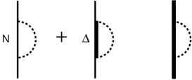
Figure 3: One-loop corrections $\Sigma^{0}_{N}$ and $\Sigma^{0}_{\Delta}$ on the nucleon and $\Delta$

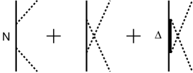
Figure 4: $\pi N$ interactions.

Taking the expectation value of $H^{P}_{2}$ between two $\pi N$ states, we then generate the $\pi N$ potential $v_{\pi N}$, illustrated in in Fig. 4. Extending the procedure described above to also include spin and isospin indices as well as the anti-particle components and $\rho$ meson, the matrix elements of $v_{\pi N}$ given explicitly in the SL model can then be obtained. On the other hand, the one-loop corrections $\Sigma^{0}_{N}$ and $\Sigma^{0}_{\Delta}$ are not treated explicitly in SL model.

Figure 5: Unphysical processes due to $H_{2}^{Q}$.

To determine $S_{2}$ from Eq. (13), we need to know the mechanisms contained in $H_{2}^{Q}$ defined by Eq. (11). With the solution Eq. (14) for $S_{1}$, one can easily see that $H_{2}^{Q}$ can generate the unphysical $B\rightarrow\pi\pi B$ processes illustrated in Fig. 5. With the similar procedure employed in solving Eq. (12) for $S_{1}$, we find that the solution of Eq. (13) from eliminating the unphysical processes illustrated in Fig. 5 can be written explicitly as the following operator form

$$S_{2} = -i\sum_{B^{\prime},B,\bar{B}}\int d\bm{p}d\bm{k}d\bm{k}^{\prime}\frac{F_{\pi B^{\prime},\bar{B}}(\bm{p}-\bm{k}-\bm{k}^{\prime},\bm{k}^{\prime};\bm{p}-\bm{k})F_{\pi\bar{B},B}(\bm{p}-\bm{k},\bm{k};\bm{p})}{E_{B}(\bm{p})-E_{B^{\prime}}(\bm{p}-\bm{k}-\bm{k}^{\prime})-E_{\pi}(\bm{k})-E_{\pi}(\bm{k}^{\prime})}\theta(2m_{\pi}+m_{B^{\prime}}-m_{B})$$ (17)

$${}[\frac{\theta(m_{\pi}+m_{B^{\prime}}-m_{\bar{B}})}{E_{B^{\prime}}(\bm{p}-\bm{k}-\bm{k}^{\prime})-E_{\bar{B}}(\bm{p}-\bm{k})+E_{\pi}(\bm{k}^{\prime})}(\frac{\theta(m_{\pi}+m_{\bar{B}}-m_{B})}{2}+\theta(-m_{\pi}-m_{\bar{B}}+m_{B}))$$

$$+\frac{\theta(m_{\pi}+m_{\bar{B}}-m_{B})}{E_{B}(\bm{p})-E_{\bar{B}}(\bm{p}-\bm{k})-E_{\pi}(\bm{k})}(\frac{\theta(m_{\pi}+m_{B^{\prime}}-m_{\bar{B}})}{2}+\theta(-m_{\pi}-m_{B^{\prime}}+m_{\bar{B}}))]$$

$$b^{\dagger}_{B^{\prime}}(\bm{p}-\bm{k}-\bm{k}^{\prime})b_{B}(\bm{p})a^{\dagger}_{\pi}(\bm{k}^{\prime})a^{\dagger}_{\pi}(\bm{k})+\mbox{h.c.}$$

We note that $S_{2}$ does not play any role in generating effective the Hamiltonian up to the second order in $\Gamma^{0}_{\pi B,B^{\prime}}$. But it is needed to evaluate the effective electromagnetic interaction operator defined by the term $[U^{\dagger}_{2}U^{\dagger}_{1}H_{em}U_{1}U_{2}]$ in Eq. (8).

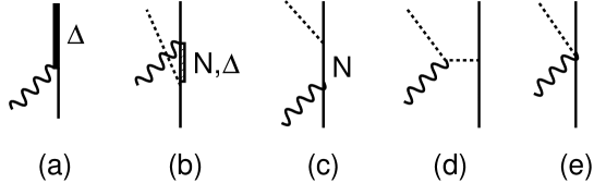
Figure 6: Leading order terms of pion photoproduction: $\Gamma^{0}_{\gamma N,\Delta}$=(a), $v^{tree}_{\gamma\pi}=(b)+(c)+(d)+(e)$

Keeping only the terms up to the same second order in $H_{I}$, we can write $[U^{\dagger}_{2}U^{\dagger}_{1}H_{em}U_{1}U_{2}]=\int d\bm{x}A\cdot J_{eff}$ with the effective current defined by

$$J^{\mu}_{eff} = J^{\mu}+[J^{\mu},iS_{1}]+\frac{1}{2}[[J^{\mu},iS_{1}],iS_{1}]+[J^{\mu},iS_{2}]+[[J^{\mu},iS_{1}],iS_{2}]\,.$$ (18)

By using the properties of $S_{1}$ and the electromagnetic coupling illustrated in Fig. 2, one can see that the first two terms of Eq. (18) for $J^{\mu}_{eff}$ generate the tree mechanisms shown in Fig. 6. Explicitly, we can see the following correspondences :

Fig. 6a $$: <\Delta\mid J^{\mu}_{\Delta,N}\mid\gamma N>,$$ (19)

$$(\mbox{Fig.6b + Fig.6c}) : <\pi N\mid[J^{\mu}_{N,N},iS_{1}]+J^{\mu}_{N,\Delta}iS_{1}\mid\gamma N>,$$ (20)

Fig.6d $$: <\pi N\mid[J^{\mu}_{\pi},iS_{1}]\mid\gamma N>,$$ (21)

Fig.6e $$: <\pi N\mid J^{\mu}_{N,N,\pi}\mid\gamma N>.$$ (22)

Extending the procedure described above to also include spin and isospin indices as well as the anti-particle components and $\rho$ and $\omega$ meson-exchange, the matrix elements for $v_{\gamma N}$ given explicitly in the SL model can then be obtained.

The one-loop corrections on the $\gamma B\rightarrow B^{\prime}$ vertex and non-resonant $\gamma N\rightarrow\pi N$ amplitude can be generated from the following operators in Eq. (18),

$$J^{\mu,1-loop}=[J^{\mu},iS_{1}]+\frac{1}{2}[[J^{\mu},iS_{1}],iS_{1}]+[J^{\mu},iS_{2}]+[[J^{\mu},iS_{1}],iS_{2}]\,.$$ (23)

For $\gamma N\rightarrow\Delta$, the possible intermediate states involved in evaluating the one-loop corrections are illustrated in Fig. 7 with the following correspondences:

Fig.7a $$: <\Delta\mid[J^{\mu}_{B^{\prime},B,\pi},iS_{1}]\mid\gamma N>,$$ (24)

Fig.7b $$: <\Delta\mid-iS_{1}J^{\mu}_{B^{\prime},B}iS_{1}\mid\gamma N>,$$ (25)

Fig.7c $$: <\Delta\mid\frac{1}{2}[[J^{\mu}_{\pi},iS_{1}],iS_{1}]+[J^{\mu}_{\pi},iS_{2}]\mid\gamma N>,$$ (26)

Fig.7d $$: <\Delta\mid\frac{1}{2}(J^{\mu}_{B^{\prime},B}iS_{1}iS_{1}+iS_{1}iS_{1}J^{\mu}_{B^{\prime},B})\mid\gamma N>.$$ (27)

Similar expressions and diagrams are also for the one-loop corrections, $<N\mid J^{1-loop}_{\mu}\mid\gamma N>$, for the nucleon electromagnetic form factors.

The one-loop corrections on the non-resonant $\gamma N\rightarrow\pi N$ amplitudes can also be obtained by taking the matrix element of $J_{\mu}^{1-loop}$ between $\pi N$ and $\gamma N$ states. We will elaborate this more complex object in section IV.

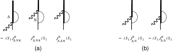
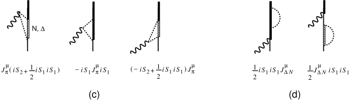
Figure 7: Loop Correction $\Gamma^{1-loop}_{\gamma N,\Delta}$ on $\gamma N\rightarrow\Delta$ transition.

With the above derivations, the effective Hamiltonian Eq. (8) within the subspace $N\oplus\Delta\oplus\pi N\oplus\gamma N$ can be written as

$$H_{eff}=[H_{0}+\Sigma^{0}_{N}+\Sigma^{0}_{\Delta}]+[\Gamma_{\pi N,\Delta}+\Gamma_{\gamma N,\Delta}]+[v_{\pi N}+v_{\gamma\pi}].$$ (28)

The mass correction terms, $\Sigma^{0}_{N}$ and $\Sigma^{0}_{\Delta}$, are illustrated in Fig. 3. The vertex interactions in Eq. (28) are

$$\Gamma_{\pi N,\Delta} = \Gamma^{0}_{\pi N,\Delta},$$ (29)

$$\Gamma_{\gamma N,\Delta} = \Gamma^{0}_{\gamma N,\Delta}+\Gamma^{1-loop}_{\gamma N,\Delta}.$$ (30)

Here we have defined

$$\Gamma^{0}_{\gamma N,\Delta}=\int d\bm{x}<\Delta\mid A\cdot J^{\mu}_{\Delta,N}\mid\gamma N>.$$ (31)

The one-loop corrections $\Gamma^{1-loop}_{\gamma N,\Delta}$ are defined by Eqs. (24)-(27) and illustrated in Fig. 7. Note that up to the second order in $H_{I}$, there is no one-loop correction to the $\pi N\rightarrow\Delta$ vertex in Eq. (29).

The $\pi N$ potential $v_{\pi N}$ in Eq. (28) is illustrated in Fig. 4. The non-resonant $\gamma N\rightarrow\pi N$ transition interaction is defined by

$$v^{\gamma\pi}=v^{tree}_{\gamma\pi}+v^{1-loop}_{\gamma\pi}$$ (32)

where $v^{tree}_{\gamma\pi}$ is defined by Eqs. (19)-(22) and illustrated in Figs. (6b)-(6d), and $v^{1-loop}_{\gamma\pi}$ is the one-loop corrections which can be calculated by taking the matrix element of Eq. (23) between $\gamma N$ and $\pi N$ states.

The SL model can be obtained from the effective Hamiltonian $H_{eff}$ of Eq. (28) by making the following simplifications. First, the mass correction terms $\Sigma^{0}_{N}$ and $\Sigma^{0}_{\Delta}$ are not treated explicitly and are included in the physical nucleon mass $m_{N}$=938.5 MeV and $m_{\Delta}=1299$ MeV determined in Ref.sl1 . Second, the one-loop corrections $\Gamma^{1-loop}_{\gamma N,\Delta}$ are not calculated explicitly and $\Gamma_{\gamma N,\Delta}$, instead of $\Gamma^{0}_{\gamma N,\Delta}$, is adjusted to fit the data. Finally, the non-resonant $v^{1-loop}_{\gamma\pi}$ is neglected.

The above derivation indicates that the method of unitary transformation has provided a systematic way to improve the SL model. In the next two sections,we will explore the consequences of these leading-order corrections derived in this section.

III One-loop corrections on the one-baryon processes

To evaluate the one-loop corrections Eqs. (15)-(16) for the baryon masses and Eqs. (24)-(27) for the $\gamma N\rightarrow N$ and $\gamma N\rightarrow\Delta$ transitions, we need to define the vertex function $F_{\pi B^{\prime},B}$ of Eq. (3) and the matrix elements of currents of Eq. (4). As an exploratory step, we assume that these can be calculated from a model within which the pion is coupled to constituent quarks by the usual pseudo-vector coupling and the electromagnetic interaction is introduced by the minimum substitution. We further assume that the constituent quarks in $N$ and $\Delta$ are nonrelativistic and only have $L=0$ s-wave configurations. Accordingly, the usual nonrelativistic limit is also taken to define the couplings of $\pi$ and $\gamma$ with constituent quarks. With these simplifications, we can cast the resulting $\pi B\rightarrow B^{\prime}$ vertex into the following form

$$F_{\pi^{i}B,B^{\prime}}(\bm{p},\bm{k};\bm{p}^{\prime})=\frac{i}{\sqrt{(2\pi)^{3}}}\frac{1}{\sqrt{2E_{\pi}(k)}}\frac{f_{\pi BB^{\prime}}}{m_{\pi}}(\bm{S}_{B^{\prime},B}\cdot\bm{k})(\bm{T}_{B^{\prime},B}\cdot\bm{I}^{i}_{\pi})F_{B^{\prime},B}(\bm{k})$$ (33)

Here $\bm{I}^{i}_{\pi}$ is a vector associated with the pion isospin state $i$, and $F_{B^{\prime},B}(\bm{k})$ is a form factor calculated from quark wave functions. The spin and isospin operators $\bm{S}_{B^{\prime}B},\bm{T}_{B^{\prime}B}$ are defined as follows. For diagonal spin operators they are twice of the spin angular momentum operator.

$$\bm{S}_{NN} = 2\bm{J}=\bm{\sigma},$$ (34)

$$\bm{S}_{\Delta\Delta} = 2\bm{J}=\bm{S}_{\Delta};$$ (35)

while the transition spin operators are defined as

$$\bm{S}_{\Delta N} = \bm{S},$$ (36)

$$\bm{S}_{N\Delta} = \bm{S}^{\dagger}.$$ (37)

Within the considered SU(6) quark model, these operators are related to each other , as given explicitly in Table I.

Table 1: Coupling constants. Here $\mu_{N}^{S}=\mu_{P}/6,\mu_{N}^{V}=5\mu_{P}/6$ with $\mu_{P}=e/2m_{q}$. $m_{q}=360$ MeV is the quark mass which is determined here by including the one-loop corrections to fit the proton magnetic moment (see Table II).

$B^{\prime}$ $B$	$\bm{S}_{B^{\prime}B}$($\bm{T}_{B^{\prime}B}$)	$<B^{\prime}||\bm{S}_{B^{\prime}B}||B>$	$f_{\pi B^{\prime}B}$	$\mu_{B}^{S}$	$\mu_{B^{\prime}B}^{V}$
$NN$	$\bm{\sigma}$	$\sqrt{6}$	$f_{\pi NN}$	$\mu_{N}^{S}$	$\mu_{N}^{V}$
$\Delta N$	$\bm{S}$	$2$	$\sqrt{72/25}f_{\pi NN}$	$0$	$\sqrt{72/25}\mu_{N}^{V}$
$N\Delta$	$\bm{S}^{\dagger}$	$-2$	$\sqrt{72/25}f_{\pi NN}$	$0$	$\sqrt{72/25}\mu_{N}^{V}$
$\Delta\Delta$	$\bm{S}_{\Delta}$	$2\sqrt{15}$	$f_{\pi NN}/5$	$\mu_{N}^{S}$	$\mu_{N}^{V}/5$

The same table also define the reduced matrix elements for isospin operators $\bm{\tau}$ for $NN$, $\bm{T}$ for $\Delta N$, $\bm{T}^{\dagger}$ for $N\Delta$, and $\bm{T}_{\Delta}$ for $\Delta\Delta$.

Let us first calculate the mass correction terms $\Sigma^{0}_{N}$ and $\Sigma^{0}_{\Delta}$ that are given in Eqs. (15)-(16). By using Eqs. (3), (14) and (33), we obtain in the rest frame of $N$ and $\Delta$

$$\Sigma^{0}_{N} = \int\frac{d\bm{k}}{(2\pi)^{3}}<m_{s_{N}}m_{\tau_{N}}\mid[(\frac{f_{\pi NN}}{m_{\pi}})^{2}\frac{1}{2E_{\pi}(\bm{k})}\frac{\bm{\sigma}\cdot\bm{k}\bm{\sigma}\cdot\bm{k}\bm{\tau}\cdot\bm{\tau}\mid F_{N,N}(k)\mid^{2}}{m_{N}-E_{\pi}(\bm{k})-E_{N}(\bm{k})}$$ (38)

$$+ (\frac{f_{\pi N\Delta}}{m_{\pi}})^{2}\frac{1}{2E_{\pi}(\bm{k})}\frac{\bm{S}\cdot\bm{k}\bm{S}^{\dagger}\cdot\bm{k}\bm{T}\cdot\bm{T}^{\dagger}\mid F_{N,\Delta}(k)\mid^{2}}{m_{N}-E_{\pi}(\bm{k})-E_{\Delta}(\bm{k})}]\mid m_{s_{N}}m_{\tau_{N}}>,$$

$$\Sigma^{0}_{\Delta} = \int\frac{d\bm{k}}{(2\pi)^{3}}<m_{s_{\Delta}}m_{\tau_{\Delta}}\mid(\frac{f_{\pi\Delta\Delta}}{m_{\pi}})^{2}\frac{1}{2E_{\pi}(\bm{k})}\frac{\bm{S}_{\Delta}\cdot\bm{k}\bm{S}_{\Delta}\cdot\bm{k}\bm{T}_{\Delta}\cdot\bm{T}_{\Delta}\mid F_{\Delta,\Delta}(k)\mid^{2}}{m_{\Delta}-E_{\pi}(\bm{k})-E_{\Delta}(\bm{k})}\mid m_{s_{\Delta}}m_{\tau_{\Delta}}>.$$

To perform the calculations, we need to define the form factor $F_{B,B^{\prime}}(\bm{k})$ in Eq. (33). To be consistent with the SL model, we here depart from the usual oscillator form and set $F_{B,B^{\prime}}(\bm{k})=(\Lambda^{2}/(\Lambda^{2}+\bm{k}^{2}))^{2}$ with $\Lambda=650$ (MeV/c)² for all $\pi BB^{\prime}$ vertices. Eqs. (38)-(LABEL:eqh39) then lead to the following results

$$\Sigma^{0}_{N} = \Sigma^{0}_{N}(\pi N)+\Sigma^{0}_{N}(\pi\Delta)$$

$$= -73.5MeV-65.4MeV=-139.MeV$$

$$\Sigma^{0}_{\Delta} = \Sigma^{0}_{\Delta}(\pi\Delta)$$ (40)

$$= -76.6MeV$$

Here we indicate the intermediate state in each pion loop term. Note that $\pi N$ intermediate state is excluded in the correction to the bare $\Delta$ mass, since its effect is already included in the rescattering term induced by the vertex interaction $\Gamma_{\pi N,\Delta}$ of Eq. (29). The contribution of this rescattering to the mass shift is

$$\Sigma^{res}_{\Delta} = P\int\frac{d\bm{k}}{(2\pi)^{3}}<m_{s_{\Delta}}m_{\tau_{\Delta}}\mid(\frac{f_{\pi N\Delta}}{m_{\pi}})^{2}\frac{1}{2E_{\pi}(\bm{k})}\frac{\bm{S}^{\dagger}\cdot\bm{k}\bm{S}\cdot\bm{k}\bm{T}^{\dagger}\cdot\bm{T}\mid F_{N,\Delta}(k)\mid^{2}}{m_{\Delta}-E_{\pi}(\bm{k})-E_{N}(\bm{k})}\mid m_{s_{\Delta}}m_{\tau_{\Delta}}>$$ (41)

$$= -46.2MeV$$

where $P$ denotes taking the principal-value part of the integration.

We now note that $(H_{0}+\Sigma^{0}_{N}+\Sigma^{0}_{\Delta})$ of the effective Hamiltonian Eq. (28) defines the physical nucleon mass and the pole position $W_{\Delta}=m_{\Delta}=1232$ MeV of the K-matrix of $\pi N$ scattering in $P_{33}$ channel. Thus, we have the following relations

$$m_{N}=m_{N}^{0}+\Sigma_{N}^{0}\,,$$ (42)

and

$$W_{\Delta}=m_{\Delta}^{0}+\Sigma_{\Delta}^{0}+\Sigma_{\Delta}^{res}\,.$$ (43)

With the above results, the mass parameters $m_{N}^{0}$ and $m_{\Delta}^{0}$ associated with $H_{0}$ of the effective Hamiltonian Eq. (28) can then be determined

$$m_{N}^{0} = m_{N}-\Sigma_{N}^{0}=1077MeV$$

$$m_{\Delta}^{0} = W_{\Delta}-\Sigma_{\Delta}^{0}-\Sigma_{\Delta}^{Res}=1355MeV$$

The difference of the two bare masses are

$$\delta^{0}=m_{\Delta}^{0}-m_{N}^{0}=278MeV$$ (44)

The mass parameters $m^{0}_{N}$ and $m^{0}_{\Delta}$ obtained above can be considered as data for determining the parameters of a hadron structure model which ‘exclude’ the pion degree of freedom. Accordingly, one can assume that $H_{0}$ of Eq. (28), which is defined by these two bare masses, can be identified with a model Hamiltonian defining the structure of the constituent quarks within the nucleon and $\Delta$.

Most of the existing constituent quark model calculationsisgu ; caps ; iach ; gloz , determine their parameters by fitting the mass difference $\delta m=m_{\Delta}(=1232)-m_{N}(=938.5)=294$ MeV, not by reproducing the absolute values of the masses of $N$ and $\Delta$. We note that this mass difference is not so different from that given in Eq. (44). Thus we can identify $H_{0}$ of Eq. (28) as the constituent quark model Hamiltonian with its eigenfunctions $\mid N>$ and $\mid\Delta>$ consisting of three quarks. Accordingly, the current matrix element $\Gamma^{0}_{\gamma N,\Delta}$ defined by Eq. (31) can be identified with the prediction from the constituent quark models.

We now turn to calculating the electromagnetic form factors. The constituent quark contribution is described by the current operator $J_{B,B^{\prime}}$ of Eq. (4). Within the considered SU(6) constituent quark model and in the second quantization notation of Eq. (3), we can write

$$\bm{J}_{B^{\prime},B} = \int\frac{d\bm{p}d\bm{p}^{\prime}d\bm{q}}{(2\pi)^{3}}[\delta(\bm{p}-\bm{q}-\bm{p}^{\prime})e^{i\bm{q}\cdot\bm{x}}b^{\dagger}_{B^{\prime}}(\bm{p}^{\prime})b_{B}(\bm{p})$$ (45)

$$\times (e[\frac{1}{2}+\frac{T_{B^{\prime},B}^{z}}{2}]\frac{\bm{p}+\bm{p}^{\prime}}{2m_{B}}\delta_{B^{\prime},B}+[\mu_{B}^{S}\delta_{B^{\prime},B}+\mu_{B^{\prime},B}^{V}T_{B^{\prime},B}^{Z}]i\bm{S}_{B^{\prime},B}\times\bm{q})F^{em}_{B^{\prime},B}(q^{2})$$

$$+(\mbox{h.c.})]$$

where $F^{em}_{B,B^{\prime}}(q^{2})$ is an electromagnetic form factor, and the parameters $\mu^{S}_{B}$ and $\mu^{V}_{B^{\prime}B}$ are defined in Table I in terms of $\mu_{P}={e}/(2m_{q})$ with $m_{q}$ denoting the quark mass. In consistent with the SL model, the other two current operators in Eq. (4) are

$$\bm{J}_{\pi} = \sum_{i,j}\int\frac{d\bm{k}d\bm{k}^{\prime}d\bm{q}}{(2\pi)^{3}}[\delta(\bm{k}-\bm{q}-\bm{k}^{\prime})e^{i\bm{q}\cdot\bm{x}}\frac{1}{\sqrt{2E_{\pi}(\bm{k})}}\frac{1}{\sqrt{2E_{\pi}(\bm{k}^{\prime})}}a^{\dagger}_{\pi^{i}}(\bm{k}^{\prime})a_{\pi^{j}}(\bm{k})$$ (46)

$$\times (-ie\epsilon_{ij3}(\bm{k}+\bm{k}^{\prime}))F^{em}_{\pi}(q^{2})+(\mbox{h.c.})]$$

and

$$\bm{J}_{B^{\prime},B,\pi} = \sum_{i,j}\int\frac{d\bm{p}d\bm{p}^{\prime}d\bm{k}d\bm{q}}{(2\pi)^{9/2}}\delta(\bm{p}-\bm{q}-\bm{p}^{\prime}-\bm{k})e^{i\bm{q}\cdot\bm{x}}\frac{1}{\sqrt{2E_{\pi}(\bm{k})}}b^{\dagger}_{B^{\prime}}(\bm{p}^{\prime})a^{\dagger}_{\pi^{i}}(\bm{k})b_{B}(\bm{p})$$ (47)

$$\times (e\frac{f_{\pi B^{\prime},B}}{m_{\pi}}\epsilon_{ij3}T_{B^{\prime},B}^{j}\bm{S}_{B^{\prime},B})F^{em}_{B^{\prime},B\pi}(q^{2})+(\mbox{h.c})].$$

The corresponding charge density operators are

$$\rho_{\pi} = \sum_{i,j}\int\frac{d\bm{k}d\bm{k}^{\prime}d\bm{q}}{(2\pi)^{3}}\frac{1}{\sqrt{2E_{\pi}(\bm{k})}}\frac{1}{\sqrt{2E_{\pi}(\bm{k}^{\prime})}}F^{em}_{\pi}(q^{2})e^{i\bm{q}\cdot\bm{x}}$$ (48)

$${}[\delta(\bm{k}-\bm{q}-\bm{k}^{\prime})a^{\dagger}_{\pi^{i}}(\bm{k}^{\prime})a_{\pi^{j}}(\bm{k})(-ie\epsilon_{ij3}(E_{\pi}(\bm{k})+E_{\pi}(\bm{k}^{\prime})))$$

$$+ \delta(\bm{k}-\bm{q}+\bm{k}^{\prime})a_{\pi^{i}}(\bm{k}^{\prime})a_{\pi^{j}}(\bm{k})(-ie\epsilon_{ij3}(E_{\pi}(\bm{k})-E_{\pi}(\bm{k}^{\prime})))+(\mbox{h.c.})],$$

$$\rho_{B^{\prime},B} = \delta_{B^{\prime},B}\int\frac{d\bm{p}d\bm{p}^{\prime}d\bm{q}}{(2\pi)^{3}}[\delta(\bm{p}-\bm{q}-\bm{p}^{\prime})e^{i\bm{q}\cdot\bm{x}}b^{\dagger}_{B^{\prime}}(\bm{p}^{\prime})b_{B}(\bm{p})e\frac{1+T^{z}_{B^{\prime},B}}{2}F^{em}_{B^{\prime},B}(q^{2})+(\mbox{h.c.})]$$ (49)

In the above equations, the form factors $F^{em}_{B^{\prime},B}(q^{2})$, $F^{em}_{\pi}(q^{2})$ and $F^{em}_{B^{\prime},B\pi}(q^{2})$ should in principle be calculated from the associated hadron structure. This is a nontrivial task, as well recognized. For this exploratory study, we simply set all of these form factors equal to $F_{V}(q^{2})=1/(1-q^{2}/M_{V}^{2})^{2}$ with $M_{V}=0.76$ GeV being the mass of vector meson. Obviously, this is the simplest prescription to maintain the gauge invariance.

With the above definitions, we can evaluate loop corrections defined by Eqs. (24)-(27) by inserting appropriate intermediate states(illustrated in Fig. 7) and using Eq. (14) for $S_{1}$ and Eq. (17) for $S_{2}$.

To proceed, we need to first fix the quark mass $m_{q}$ which determine the current $J_{B^{\prime}B}$. This is done by fitting the nucleon magnetic moments. The one-loop corrections (similar to what are shown in Fig. 7) are included in the fit. We find that the nucleon magnetic moments can be reproduced very well if we set the quark mass as $m_{q}=360$ MeV. The results for the magnetic moments are shown in Table II. We see that the loop corrections are about 5$\%$ for proton and 10 $\%$ for neutron.

Table 2: Magnetic moment of nucleon in unit $\mu_{N}$

	’tree’	Total with loop corrections
proton	2.61	2.75
neutron	-1.74	-1.95

It is important to note that the size of one-loop corrections depend heavily on the range $\Lambda$ of the form factor $F_{B^{\prime},B}$ of Eq. (33).

We now turn to investigating the loop corrections on the $\gamma N\rightarrow\Delta$ transition. Following the formulation presented in SL model, the $\gamma N\rightarrow\Delta$ vertex function calculated in the $\Delta$ rest frame can be written in the following form

$$<\Delta\mid\Gamma_{\gamma N\rightarrow\Delta}\mid q> = -\frac{e}{(2\pi)^{3/2}}\sqrt{\frac{E_{N}(\bm{q})+m_{N}}{2E_{N}(\bm{q})}}\frac{1}{\sqrt{2\omega}}\frac{3(m_{\Delta}+m_{N})}{4m_{N}(E_{N}(\bm{q})+m_{N})}T_{3}$$ (50)

$$\times {}[iG_{M}(q^{2})\bm{S}\times\bm{q}\cdot\bm{\epsilon}+G_{E}(q^{2})(\bm{S}\cdot\bm{\epsilon}\bm{\sigma}\cdot\bm{q}+\bm{S}\cdot\bm{q}\bm{\sigma}\cdot\bm{\epsilon})$$

$$+\frac{G_{C}(q^{2})}{m_{\Delta}}\bm{S}\cdot\bm{q}\bm{\sigma}\cdot\bm{q}\epsilon_{0}],$$

where $e=\sqrt{4\pi/137}$, $q=(\omega,\bm{q})$ is the photon four-momentum, and $\epsilon=(\epsilon_{0},\bm{\epsilon})$ is the photon polarization vector. The above definition allows us to calculate the multipole amplitudes of the $\gamma N\rightarrow\Delta$ in terms of $G_{M}(q^{2})$, $G_{E}(q^{2})$ and $G_{C}(q^{2})$. Explicitly, we havesl2

$$A_{M}(q^{2}) = [\Gamma_{\gamma N\rightarrow\Delta}]_{M1}=NG_{M}(q^{2})$$ (51)

$$A_{E} = [\Gamma_{\gamma N\rightarrow\Delta}]_{E2}=-NG_{E}(q^{2})$$ (52)

$$A_{C} = [\Gamma_{\gamma N\rightarrow\Delta}]_{C2}=N\frac{\mid\bm{q}\mid}{2m_{\Delta}}G_{C}(q^{2}),$$ (53)

with

$$N=\frac{e}{2m_{N}}\sqrt{\frac{m_{\Delta}\mid\bm{q}\mid}{m_{N}}}\frac{1}{[1-q^{2}/(m_{N}+m_{\Delta})^{2}]^{1/2}}$$ (54)

We first discuss the results at $q^{2}=0$ photon point. The values of $A_{M}$, $A_{E}$, and $A_{C}$ determined in Refs.sl1 ; sl2 are listed in Table III. These are the quantities we would like to interpret within the considered constituent quark model. Assuming that $\Gamma_{\gamma N,\Delta}$ of Eq. (30) is what has been determined in the SL model, the values listed in Table III thus include the contribution not only from the quark-excitation term $\Gamma^{0}_{\gamma N,\Delta}$ of Eq. (31), which can be calculated from Eqs. (45) and (49), but also include the pion-loop contributions illustrated in Fig. 7. These loop contributions can be calculated by inserting appropriate intermediate states in the commutators of Eqs. (24)-(25). As an example, we write down the expression for the mechanism Fig. 7b in the rest frame of $\Delta$ ($\bm{p}_{\Delta}=0$, $\bm{p}_{N}=-\bm{q}$)

$$<\Delta|-iS_{1}J^{\mu}_{B^{\prime},B}iS_{1}|N> =\int d\bm{k}\sum_{B=N,\Delta}$$ (55)

$$\frac{<\Delta|\Gamma^{0\dagger}_{\pi\Delta,\Delta}|\pi(\bm{k}),\Delta><\Delta|J^{\mu}_{\Delta,B}|B><\pi(\bm{k}),B|\Gamma^{0}_{\pi B,N}|N>}{(m_{\Delta}-E_{\Delta}(\bm{k})-E_{\pi}(\bm{k}))(E_{N}(\bm{q})-E_{B}(\bm{q}+\bm{k})-E_{\pi}(\bm{k}))}$$

$$=\int d\bm{k}\sum_{B=N,\Delta}$$

$$\frac{F_{\pi\Delta,\Delta}^{\dagger}(0,-\bm{k},\bm{k})<\Delta|J^{\mu}_{\Delta,B}|B>F_{\pi B,N}(-\bm{k}-\bm{q},-\bm{q},\bm{k})}{(m_{\Delta}-E_{\Delta}(\bm{k})-E_{\pi}(\bm{k}))(E_{N}(\bm{q})-E_{B}(\bm{q}+\bm{k})-E_{\pi}(\bm{k}))}$$

An important point to note here is that the integrand in the loop-integration is independent of the collision energy $W$ and has no singularity in the integration region $0\leq k\leq\infty$. Thus the included pion cloud effects are different from what were calculated from the SL model : $[v_{\gamma\pi}G_{\pi N}(W)\bar{\Gamma}_{\pi N,\Delta}(W)]$ which depends on the collision energy $W$ in the $\pi N$ propagator $G_{\pi N}(W)$. Qualitatively speaking, the one-loop contributions of Fig. 7 are due to virtual pions which are part of the internal structure of N or $\Delta$, while the SL model only accounts for the effects due to pions in scattering states which can reach the on-shell momentum asymptotically.

The $Q^{2}=0$ ($Q^{2}=-q^{2}>0)$ results from our complete calculations for all one-loop terms in Fig. 7 are presented in Table IV. In the first row, we list the values from $\Gamma_{\gamma N\rightarrow\Delta}^{0}$, which is due to photon interactions with constituent quarks. As expected, the assumed spherical s-wave quark configurations do not have $E2$ and $C2$ transitions. In the same table we also list the contribution from each loop contribution illustrated in Fig. 7. The terms under ’pion’ and ’Seagull’ are from Fig. 7a and 7c respectively. Fig. 7d gives the contribution ’Normalization’ which is the consequence of the appearance of the mass shifts $\Sigma^{0}_{N}$ and $\Sigma^{0}_{\Delta}$ in the effective Hamiltonian Eq. (30) and is naturally derived here by using the unitary transformation method. Fig. 7b contains the contributions due to spin transition and convection current. Their separate contributions are listed under ’Spin’ and ’Convection’ respectively. We note that $A_{C}$ only has contribution from pion term because of the angular moment selection rule.

We should emphasize here that the present calculations are based on a non-relativistic quark model and can only be compared qualitatively with the empirical values (table III) determined in the SL model. Thus we should not worry about their differences in absolute magnitudes. Rather, we focus on the relative importance between $A_{M}$, $A_{E}$ and $A_{C}$ listed in Tables III and IV.

The first interesting result in Table IV is that the total one-loop correction (Total - $\Gamma^{0}_{\gamma N,\Delta}$) for the magnetic form factor $G_{M}$ is only about 4 $\%$ of the ’bare’ value $\Gamma^{0}_{\gamma N,\Delta}$, mainly due to the large cancellations between different contributions. In particular, the very large contribution from ’Normalization’ of Fig. 7d plays a crucial role. We also see that the calculated $A_{E}$ and $A_{C}$ in Table IV are in opposite signs of the values listed in Table III. These results have the following implications. First, the $\Gamma^{0}_{\gamma N,\Delta}$ values of $A_{E}$ and $A_{M}$ in Table IV could be nonzero and negative such that the total values become the SL values listed in Table III. This can be the case if we assume that the quark wavefunctions of $\Delta$ and/or $N$ could have a $L=2$ d-state component. The other possibilities are that there could have multi-pion loop corrections and exchange current contribution of the quark electromagnetic currentbuchmann . Within our formulation, some of these mechanisms can be derived from applying the third-order unitary transformation $U_{3}$. A more detailed study along this line is clearly needed to make progress.

Table 3: ’bare’ helicity amplitudes of the SL model[1,2]. Unit is $10^{-3}GeV^{-1/2}$.

$A_{M}$	173.3
$A_{E}$	-2.3
$A_{C}$	-2.2

Table 4: ’bare’ helicity amplitudes in quark model with loop correction. Unit is $10^{-3}GeV^{-1/2}$. SL is the result from Ref.[1,2]

	$\Gamma^{0}_{\gamma N,\Delta}$		Pion		Spin		Convection		Seagull		Normalization		Total
$A_{M}$	204.9		23.7		24.2		0		-3.3		-35.6		213.8
$A_{E}$	0		2.8		-0.1		0.1		0.9		0		3.6
$A_{C}$	0		1.1		0		0.0		0		0		1.1

The calculated $Q^{2}-$ dependence of the $\gamma N\rightarrow\Delta$ form factors are displayed in Figs. 8 and 9. The dominant M1 transition is shown in Fig. 8. The difference between the solid and dashed curves is due to the one-loop corrections. It is very weak and only visible at very low $Q^{2}$. On the other hand, the pion cloud effects due to scattering states (dashed curve) is very large, As discussed in detail in Ref. sl2 , this finding explains why the conventional constituent quark model predictions disagree with the empirical value of the magnetic M1 transition of $\gamma N\rightarrow\Delta$. The present result for one-loop corrections do not change that conclusion.

The situation for $A_{E}(Q^{2})$ and $A_{C}(Q^{2})$ is quit different. Here we do not have contribution from quark excitation term $\Gamma^{0}_{\gamma N,\Delta}$ because of the assumed L=0 wavefunctions. We see that the calculated one-loop corrections (solid curves) are comparable in magnitudes to the pion cloud effects due to scattering state (dashed curves) calculated in SL model. More importantly, they have very different $Q^{2}$-dependence and are opposite in signs. As seen in Eq. (30), the solid curves must be interpreted as part of the bare form factors determined phenomenologically in SL model. Namely, the form factors obtained from subtracting the solid curves from SL model’s bare form factors are the contribution from quark excitation. This will be an important information for testing various hadron structure calculations. However, such information can not be realistically extracted here because of the simplicity of the model employed.

Figure 8: $A_{M}(Q^{2})$. Dot-dashed is from quark excitation $\Gamma^{0}_{\gamma N,\Delta}$, the solid curve is the sum of $\Gamma^{0}_{\gamma N,\Delta}$ and $\Gamma^{1-loop}_{\gamma N,\Delta}$. The dashed curve is from pion scattering calculated in SL model.

Figure 9: Left:$A_{E}(Q^{2})$, Right:$A_{C}(Q^{2})$. Solid curves are from one-loop corrections, while the dashed curves are from pion scattering calculated in SL model.

IV One-loop corrections on non-resonant $\gamma N\rightarrow\pi N$

One of the difficulties the SL model has in describing the data is from the non-resonant amplitude. In this section, we would like to explore whether this can be improved by including the one-loop corrections $v^{1-loop}_{\gamma\pi}$ of Eq. (32). As a start, we will focus on the near threshold region and consider only the the $E_{0+}$ amplitude. A complete calculation of $v^{1-loop}_{\gamma\pi}$ for all partial waves up to $\Delta$ resonance energy is much more involved and will be explored elsewhere.

First, we point out that the SL model failed to describe the near threshold $\gamma p\rightarrow\pi^{0}p$ data. For example, at $E_{\gamma}=145$ MeV the SL model gives (after taking into account the effects due to the mass difference between $\pi^{0}$ and $\pi^{\pm}$ )

$$E_{0+}(145{\it MeV})=-2.47(Born)+2.31(Rescattering)=-0.15[10^{-3}/m_{\pi^{+}}]$$ (56)

where $Born$ is from the non-resonant production operator $v^{tree}_{\gamma\pi}$ constructed in SL model, $Rescattering$ include the effects due to final $\pi N$ interaction. The empirical value is $E_{0+}^{exp}$ (145 MeV) $\sim$ -1.50. In getting the above result, we find that the main contributions to the Born term are from the nucleon-direct and nucleon-exchange diagrams, while the rescattering term is mainly from pion-pole and contact interaction through $\gamma+p\rightarrow\pi^{+}+n\rightarrow\pi^{0}+p$ charge-exchange process. We also find that the s-wave charge exchange pion rescattering is dominated by the $\rho$-exchange $\pi-N$ potential and the Born approximation $t_{\pi N}\sim v_{\pi N}$ is accurate. Furthermore the short range approximation of $\rho$-exchange potential ($1/(m_{\rho}^{2}+(\bm{p}_{N}-\bm{p}^{\prime}_{N})^{2})\sim 1/m_{\rho}^{2}$) is accurate within 10% in determining the rescattering effects in the considered near threshold energy region. With these considerations, the one-loop corrections near threshold can be calculated with the following much simplified Hamiltonian

$$H_{I} = \frac{f_{\pi NN}}{m_{\pi}}\bar{\psi}_{N}\gamma_{5}\gamma_{\mu}\partial^{\mu}\vec{\phi}_{\pi}\cdot\vec{\tau}\psi_{N}+\lambda\bar{\psi}_{N}\gamma^{\mu}\vec{\tau}\psi_{N}\cdot\vec{\phi}_{\pi}\times\partial_{\mu}\vec{\phi}_{\pi}\,.$$ (57)

Here the second term is a contact interaction with the strength determined from the $\rho$-exchange coupling constants : $\lambda=g_{\rho\pi\pi}g_{\rho NN}/(2m_{\rho}^{2})$. By minimum substitution, the second term of Eq. (57) will generate a interaction current

$$j^{\mu}_{N,N\pi\pi} = e\lambda[\bar{\psi}_{N}\gamma^{\mu}\vec{\tau}\psi_{N}\times\vec{\phi}_{\pi}]\times\vec{\phi}_{\pi}\,.$$ (58)

It induces an electromagnetic contact interaction involving two pions. To maintain the gauge invariance within the model defined by the simplified interaction Hamiltonian Eq. (57), this current is included in the calculation along with the currents $J_{\pi}$, $J_{B^{\prime},B}$ and $J_{B^{\prime},B\pi}$ given in Eqs. (46)-(48) and illustrated in Fig. 2. All coupling constants and vertex form factors are taken from SL model.

With the above simplified model, we first re-calculate the rescattering contributions, $\sim v^{tree}_{\gamma,\pi}G_{\pi N}(W)v_{\pi N}$ to the $E_{0^{+}}$ amplitude for $\gamma p\rightarrow\pi^{0}p$. The results at $E_{\gamma}=145$ MeV are listed in Table V. It is instructive to note here that the calculated rescattering contribution involves cancellation between the terms (d) and (e). The total rescattering value 2.36 is very close to the value 2.31 of the rescattering term in Eq. (56) of the SL model. This justifies the use of the simplified model defined by Eqs. (57) and (58).

Table 5: Rescattering contributions to the $E_{0^{+}}$ amplitude of $\gamma p\rightarrow\pi^{0}p$ at 145 MeV, calculated from mechanisms (b)-(e) illustrated in Fig. 6 using the model defined by Eqs. (57)-(58).

Diagram			(b)			(c)			(d)			(e)			sum
			-0.074			-0.685			-1.966			5.087			2.36

Figure 10: Subset of loop corrections on the $\gamma N\rightarrow\pi N$ transition amplitude.

Figure 11: Subset of Loop corrections on the $\gamma N\rightarrow\pi N$ transition amplitude.

The one-loop corrections can be calculated from Eq. (23) by inserting appropriate intermediate states. The resulting amplitudes are illustrated in Figs. 10 and 11. Note that diagrams in Figs. 10 and 11 are not time-ordered diagrams. Rather they just illustrate the structure of the matrix element of each term in $v^{1-loop}_{\gamma\pi}$. As seen from Eq. (14) and Eq. (17), the loop integrations for all processes in Figs. 10 and 11 will involve $energy-independent$ propagators associated with these two operators. Thus, although the diagrams in Fig. 10 look similar to the rescattering terms, but they are $energy-independent$ matrix elements. The calculations for these loops are tedious but straightforward, and will not be elaborated here.

Table 6: one-loop contributions to the $E_{0^{+}}$ amplitude of $\gamma p\rightarrow\pi^{0}p$ at 145 MeV, calculated from mechanisms illustrated in Fig. 11 using the model defined by Eqs.(54).

	Diagram			$E_{0+}$			Diagram			$E_{0+}$
Fig. 10	(a)			-0.079			(c)			-0.024
	(b)			-0.090			(d)			0.475
Fig. 11	(a)			0.157			(f)			-0.418
	(b)			-1.192			(g)			0.00
	(c)			0.875			(h)			0.00
	(d)			-0.085			(i)			-0.696
	(e)			-1.011			(j)			0.699
							Sum = -1.39

Our results at $E_{\gamma}=145$ MeV for each of the one-loop corrections shown in Figs. 10 and 11 are listed in Table VI. The results listed in Tables V and VI lead to

$$E_{0+}(145MeV)=-2.47(Born)+2.32(Rescattering)-1.39(Loop)=-1.54$$ (59)

This reproduces the empirical value $E_{0+}^{exp}$ (145 MeV) $\sim$ -1.50. The calculated effect of the one-loop corrections for $E_{0+}$ in the near threshold energy region is shown in in Fig. 12. Clearly, the one-loop corrections drastically reduce the magnitudes and bring the results to agree with the empirical values. The kinks due to the cups effect are reproduce well in our calculations.

Figure 12: $E_{0+}$ amplitude of $\gamma p\rightarrow\pi^{0}p$. The dotted curve is from $v^{tree}_{\gamma\pi}$. The solid curves are obtained when the one-loop corrections $v^{1-loop}_{\gamma\pi}$ are included. The data are from Refs e0exp1 ; e0exp2 ; e0exp3

In Fig. 13, we show that the one-loop corrections on the $E_{0^{+}}$ amplitude can change significantly the calculated angular distributions to better agree with the data. To see the full one-loop correction effects, we need to also calculate other multipole amplitudes. This along with the results for the $\Delta$ region will be explored elsewhere.

Figure 13: $\gamma p\rightarrow\pi^{0}p$ at 146, 150, 160, and 170 MeV. Solid curves are obtained when the one-loop corrections $v^{1-loop}_{\gamma\pi}$ are included. Data are from Ref.e0exp1 ; e0exp2 .

V Summary and Outlook

In this paper, we have applied the unitary transformation to derive the leading-order corrections on the effective Hamiltonian of the SL model for electromagnetic pion production reactions. We have investigated the one-loop corrections on the masses of $N$ and $\Delta$, the $\gamma N\rightarrow\Delta$ vertex, and the non-resonant pion production operators. Qualitatively speaking, the derived one-loop corrections are due to the virtual pions which are part of the internal structure of $N$ or $\Delta$, while the pion cloud effects generated within the SL model or the other dynamical models, such as the Dubna-Mainz-Taipei (DMT) model dmt , only account for the effects due to pions in the scattering states which can reach the on-shell momentum asymptotically.

With the one-loop corrections included in determining the mass parameters, we find that the free Hamiltonian of the model can be identified with the conventional constituent quark model. We then proceed to apply such a constituent quark model to calculate the one-loop corrections on the $\gamma N\rightarrow\Delta$ transition form factors. It is found that the one-loop corrections on the magnetic M1 transition is very small. Our results further establish the conclusion reached by the SL model that the large discrepancy between the conventional constituent quark model predictions and the empirical values are due to the pion cloud effects associated with the pions in scattering states.

The calculated one-loop contributions to the electric E2 ($A_{E}$) and Coulomb C2 ($A_{C}$) form factors of the $\gamma N\rightarrow\Delta$ transition are found to be in opposite signs of that due to pion cloud associated with the scattering states. One possible implications of this result is that the extracted empirical values of SL model could be largely due to the nonspherical $L=2$ intrinsic quark excitations which could lead to nonzero and negative contributions to $A_{E}$ and $A_{C}$. On the other hand, there could have higher-order exchange current contributions which are not included in this work, but must be also calculated for a complete understanding of the empirical values of SL model. Clearly more works are highly desirable.

We have also found that the one-loop corrections on the non-resonant pion production operator can resolve the difficulty the SL model encountered in reproducing the empirical $E_{0+}$ amplitude of near threshold $\pi^{0}$ photoproduction. It will be worthwhile to further extend this work to calculate these one-loop corrections for higher partial waves. Some of the discrepancies between the SL model and the data in the $\Delta$ excitation could be removed by including these corrections. Our effort in this direction will be reported elsewhere.

To end, we emphasize that the SL model is obtained from keeping only the lowest order terms of a formulation within which the higher order terms can be rigorously derived. Attempts to fit the data by adjusting the current SL model are not justified theoretically. The most important task to improve the SL model is to include these corrections order by order until the convergence of the predictions has achieved. In this work we have taken a very first step in this direction. Undoubtly, much more works are needed to complete a consistent dynamical model of electromagnetic pion production reactions.

This work was supported by the U.S. Department of Energy, Office of Nuclear Physics Division, under contract no. W-31-109-ENG-38, and by Japan Society for the Promotion of Science, Grant-in-Aid for Scientific Research (C) 15540275.

References

- (1) See a review by V. Burkert and T.-S. H. Lee, to appear in Jour. of Modern Physics E (2004).
- (2) T. Sato and T.-S. H. Lee, Phys. Rev. C 54, 2660 (1996).
- (3) T. Sato and T.-S. H. Lee, Phys. Rev. C 63, 055201 (2001).
- (4) Kamalov and S.N. Yang, Phys. Rev. Lett. 83, 4494 (1999).
- (5) S.S. Kamalov, S. N. Yang, D. Drechsel, O. Hanstein, and L. Tiator, Phys, Rev, C64, 032201(R) (2001).
- (6) D. Drechsel, O. Hanstein, S.S. Kamalov, and L. Tiator, Nucl. Phys. A645, 145 (1999).
- (7) M. Kobayashi, T. Sato and H. Ohtsubo, Prog. Theor. Phys. 98, 927 (1997).
- (8) H. M. Nieland and J.A. Tjon, Phys. Lett. 27B,309 (1968).
- (9) A.D. Lahiff and I.R. Afnan, Phys. Rev. C60, 024608 (1999).
- (10) B.C. Pearce and B.K. Jennings, Nucl. Phys. A528, 655 (1991).
- (11) F. Gross and Y. Surya, Phys. Rev. C47, 703 (1993); Y. Surya and F. Gross, ibid., C53, 2422 (1996).
- (12) C. Schutz, J. W. Durso, K. Holinde, and J. Speth, Phys. Rev. C 49, 2671 (1994).
- (13) C. T. Hung, S. N. Yang, and T.-S. H. Lee, Phys. Rev. C 64, 034309 (2001); J. Phys. G 20, 1531 (1994).
- (14) V. Pascalutsa and J.A. Tjon, Phys. Rev. C61, 054003 (2000).
- (15) N. Isgur and G. Karl, Phys. Rev. D 18, 4187 (1978); Phys. Rev. D 19, 2653 (1979).
- (16) S. Capstick, Phys. Rev. D 46, 1965 (1992); Phys. Rev. D 46, 2864 (1992).
- (17) R. Bijker, F. Iachello, and A. Leviatan, Amm. Phys.(N.Y.) 236, 69 (1994).
- (18) L. Ya. Glozman and D. O. Riska, Phys. Rep. 268, 263 (1996); L. Ya. Glozman, Z. Rapp, W. Plessas, K. Varga, and R. F. Wagenbrunn, Nucl. Phys. A623, 90c (1997).
- (19) A. J. Buchmann, E. Hernandez and A. Faessler, Phys. Rev. C55, 448 (1997).
- (20) M. Fuchs et al., Phys. Lett. B368, 20 (1996).
- (21) J. C. Bergstrom et al., Phys. Rev. C55, 2016 (1997).
- (22) A. Schmidt et al., Phys. Rev. Lett. 87, 232501 (2001).