Statistical hadronization with resonances

Abstract

We introduce the equilibrium and non-equilibrium statistical hadronization picture of particle production in ultra-relativistic heavy ion collisions. We describe the related physical reaction scenarios, and show how these can lead to quark pair yield non-equilibrium. Using the SHARE1.2 program suite we quantitatively model particle yields and ratios for RHIC-130 run. We study how experimental particle ratios can differentiate between model scenarios, and discuss in depth the importance of hadronic resonances in understanding of hadron production processes.

1 Introduction

In strong interaction reaction processes particle production is abundant. In the Fermi-Hagedorn statistical model the non-perturbative description of particle yields is based on the assumption that particle production is governed solely by the size of the accessible phase space. For an introduction into the literature and history of the statistical hadronization model we refer the reader to Ref. [1]. Further recent developments are discussed in [2, 3]. We focus in this report on current developments related to RHIC experimental program, involving the measurement of hadron yields, obtained by integrating the produced stable particle spectra.

The statistical hadronization picture is necessarily an integral part of the modeling of this“soft” experimental hadron production data. This is both to provide a bottom line to eventual microscopic production mechanisms signaling new physics, and to search for abrupt changes associated with a phase transformation in which hadrons dissolve into a phase of quarks and gluons.

Hagedorn [4] was first to recognize the importance of hadronic resonances in statistical particle production. To quantitatively describe hadron final state yields, contributions from resonance decays must be taken into account. As it turns out, the effect of these resonance decays on particle phase space is crucial: As Hagedorn has shown, it can be expected that the density density of states of strongly interacting resonances increases exponentially with energy,

$$\rho(E)\sim e^{\beta_{\rm H}E}$$ (1)

This has a profound implications for the behavior of matter at high temperature. It leads to a phase singularity at the temperature (“Hagedorn Temperature”, $T_{\rm H}=\beta_{\rm H}^{-1}\approx 160$ MeV) where the canonical partition function diverges:

$$Z=\sum_{i}\rho(E_{i})e^{-E_{i}/T}\left.\right|_{T\to T_{\rm H}}\to\infty.$$ (2)

Hagedorn referred to this as the boiling point of hadronic matter. With advancement of the quark picture of matter he recognized this singularity as being the deconfinement transition, where hadrons cease to be fundamental degrees of freedom, and quarks are able to propagate freely throughout the system.

Currently, an intense experimental effort (covering an energy range from 2 to 200 GeV) is underway to create, and identify, a relatively large volume of deconfined quark–gluon matter, the quark–gluon plasma (QGP), and to explore its properties. In the following section we describe in turn within the statistical hadronization model: particle and quark chemistry in subsection 2.1, resonance decay chains in subsection 2.2, and we introduce the finite resonance widths in subsection 2.3. The reader is referred to Refs. [5] – [20] for many further details. In subsection 2.4 we discuss in some detail how it is possible that chemical non-equilibrium occurs in a strongly interacting system. We than turn to the more phenomenological aspects, and introduce the practical aspects of the statistical model in section 3 where we also develop strategies for detecting chemical nonequilibrium. In section 4 we discus the fitting method and proceed to present some RHIC related results obtained with the SHARE suite of programs.

2 The statistical particle production model

2.1 Particle chemistry and yields in the statistical model

In the grand canonical description the expected baryon and meson yields are given by the Fermi-Dirac or, respectively, Bose-Einstein distribution functions:

$$n(m_{i},g_{i};T,\Upsilon_{i})\equiv n_{i} = g_{i}\int{d^{3}p\over(2\pi)^{3}}{1\over\Upsilon^{-1}_{i}\exp(\sqrt{p^{2}+m^{2}_{i}}/T)\pm 1},$$ (3)

$$= \frac{g_{i}}{2\pi^{2}}\sum_{n=1}^{\infty}(\mp)^{n-1}\Upsilon_{i}^{n}\,\frac{T\,m_{i}^{2}}{n}\,K_{2}\left(\frac{nm_{i}}{T}\right).$$ (4)

In the upper signs refer to fermions and the lower signs to bosons, respectively. The second form, Eq. (4), expresses the momentum integrals in terms of the modified Bessel function $K_{2}$. This form is practical in the numerical calculations. The series expansion (sum over $n$) converges when $\Upsilon_{i}e^{-m_{i}/T}<1$, below the Bose-Einstein condensation limit. Consideration of this condition is required only for the pion yield in the range of parameters of interest. Here, the index ‘$i$’ labels different particle species, including hadrons which are stable under strong interactions (such as pions, kaons, nucleons or hyperons) and hadron which are unstable ($\rho$ mesons, $\Delta(1232)$, etc.). $m_{i}$ is the particle mass, while the quantity $g_{i}=(2J_{i}+1)$ is the spin degeneracy factor; we will distinguish all isospin sub-states separately.

$\Upsilon_{i}$ is the fugacity factor. Since particle anti-particle pairs ($i\overline{i}$) can be produced by particles without conserved ‘charges’ (baryon number, strangeness, etc.),

$$i+\overline{i}\rightleftharpoons n\times\gamma,g,\pi,...\mathrm{(n-objects\;\;with\;\;no\;\;conserved\;\;charges)}$$ (5)

a scenario where statistical production arises as a limit of kinetic evolution requires that the chemical potentials of particles and antiparticles associated with the conserved charge be opposite. Thus the fugacity $\Upsilon_{i}$ comprises the well known factor $\lambda^{\pm 1}=e^{\pm\mu/T}$, where $\mu$ is the chemical potential associated with a conserved quantum number.

For a dynamically evolving system yield of particles cannot in general be in chemical equilibrium. This is accommodated by introducing a phase space occupancy factor $\gamma$:

$$\Upsilon_{j}=\gamma_{j}\lambda_{j},\qquad\Upsilon_{\overline{j}}=\gamma_{j}\lambda_{j}^{-1}$$ (6)

$\gamma_{j}=1$ corresponds to chemical equilibrium. $\gamma_{j}<1$ means that quantum number $j$ is under-saturated, usually because time is needed to build it up. An isolated system kept long enough “in a box” would generate more of $j\overline{j}$ particle-antiparticle pairs at the expense of the internal energy. If this equilibrated box undergoes isentropic and rapid expansion ($VT^{3}=\mbox{Const.}$ for massless particles), $\gamma_{j}>1$ will generally result as the particle abundances do not have time to re-equilibrate [21]. Given time in the “large box”, pairs would annihilate and the system would again relax to an equilibrium state. In subsection 2.4 we will explore these scenarios more thoroughly, and in section 3 we will argue that equilibrium assumptions can and should be tested against experimental data.

Each hadron can be a carrier of several conserved charges contained in its valance quarks. The most general fugacity $\Upsilon_{j}$ for hadron $j$ is given by a suitable product of $\lambda$ and $\gamma$ factors:

$$\Upsilon_{j}=\lambda_{I^{j}_{3}}\left(\lambda_{q}\gamma_{q}\right)^{N^{j}_{q}}\left(\lambda_{s}\gamma_{s}\right)^{N^{j}_{s}}\left(\lambda_{c}\gamma_{c}\right)^{N^{j}_{c}}\left(\lambda_{\bar{q}}\gamma_{\bar{q}}\right)^{N^{j}_{\bar{q}}}\left(\lambda_{\bar{s}}\gamma_{\bar{s}}\right)^{N^{j}_{\bar{s}}}\left(\lambda_{\bar{c}}\gamma_{\bar{c}}\right)^{N^{j}_{\bar{c}}},$$ (7)

where

$$\lambda_{q}=\lambda^{-1}_{\bar{q}},\qquad\lambda_{s}=\lambda^{-1}_{\bar{s}},\qquad\lambda_{c}=\lambda^{-1}_{\bar{c}},\qquad$$ (8)

and

$$\gamma_{q}=\gamma_{\bar{q}},\qquad\gamma_{s}=\gamma_{\bar{s}},\qquad\gamma_{c}=\gamma_{\bar{c}}.$$ (9)

Here, $N^{j}_{q}$, $N^{j}_{s}$ and $N^{j}_{c}$ are the numbers of light $(u,d)$, strange $(s)$ and charm $(c)$ valance quarks in the $j$th hadron, and $N^{j}_{\bar{q}}$, $N^{j}_{\bar{s}}$ and $N^{j}_{\bar{c}}$ are the numbers of the corresponding valance antiquarks in the same hadron.

The quark and hadron chemical potentials as used in e.g. Refs. [12, 22, 23] are related by simple algebraic conditions arising from the valance quark content and definitions of the baryon and hyperon charges of particles given in the historical context. Considering the case of chemical equilibrium limit $\gamma_{q}=\gamma_{s}=1$ and in absence of charm ($N^{i}_{c}=N^{i}_{\bar{c}}=0$):

$$\Upsilon^{\rm\,\,eq}_{i}=\exp\left(\frac{B_{i}\mu_{B}+S_{i}\mu_{S}+I^{\,i}_{3}\mu_{I_{3}}}{T}\right),$$ (10)

where $B_{i}$, $S_{i}$, and $I^{\,i}_{3}$ are the baryon number, strangeness, and the third component of the isospin of the $i$th particle, and $\mu$’s are the corresponding chemical potentials. In this case, the two formulations are related by equations:

$$\lambda^{\rm eq}_{q}=e^{\mu_{B}/3T},\,\,\,\,\,$$ (11)

$$\lambda^{\rm eq}_{S}=e^{(-3\mu_{s}+\mu_{B})/3T},\,\,\,\,\,$$ (12)

$$\lambda^{\rm eq}_{I^{i}_{3}}=\lambda_{I^{i}_{3}}=e^{I^{\,i}_{3}\mu_{I_{3}}/T}.$$ (13)

We note that strangeness and hyperon number $S$ of a particle are by historical convention opposite in sign to each other,

$$\mu_{S}=\mu_{s}-\mu_{q}.$$

Since we use the symbol $S$ also for entropy, henceforth we will refrain from mentioning the hyperon number.

2.2 Resonance decays

In the first instance, we consider hadronic resonances as if they were particles with a given well defined mass, e.g., their decay width is insignificant. All hadronic resonances decay rapidly after freeze-out, feeding the stable particle abundances. Moreover, heavy resonances may decay in cascades, where all decays proceed sequentially from the heaviest to lightest particles. As a consequence, the light particles obtain contributions from the heavier particles, which have the form

$$n_{1} = b_{2\rightarrow 1}\,...\,b_{N\rightarrow N-1}n_{N},$$ (14)

where $b_{k\rightarrow k-1}$ combines the branching ratio for the $k\rightarrow k-1$ decay (appearing in [24]) with the appropriate Clebsch–Gordan coefficient. The latter accounts for the isospin symmetry in strong decays and allows us to treat separately different charged states of isospin multiplets of particles such as nucleons, Deltas, pions, kaons, etc. For example, different isospin multiplet member states of $\Delta$ decay according to the following pattern:

$$\Delta^{++}\rightarrow\pi^{+}+p,$$ (15)

$$\Delta^{+}\rightarrow{1\over 3}(\pi^{+}+n)+{2\over 3}(\pi^{0}+p),$$ (16)

$$\Delta^{0}\rightarrow{1\over 3}(\pi^{-}+p)+{2\over 3}(\pi^{0}+n),$$ (17)

$$\Delta^{-}\rightarrow\pi^{-}+n.$$ (18)

Here, the branching ratio is 1 but the Clebsch–Gordan coefficients introduce another factor leading to the effective branching ratios of 1/3 or 2/3, where appropriate.

A decay such as $\Delta\longrightarrow\pi N$ is easy to deal with, since only one decay channel is present and the branching ratio is well known. However, for most of the resonances several decay channels appear and the partial widths (product of branching ratio with total width) are in general less well known, usually classified as dominant, large, seen, or possibly seen, [24]). Any statistical hadronization calculation where high-lying massive states are relevant should carefully consider the dependence of this uncertainty in its results, especially considering the increasing resonance degeneracy with mass [25].

Weak hadron decays complicate the physics of hadron yield and spectra study considerably. The weak interaction life span for strange hadrons (excluding $K_{L}$) ranges in 2–10 cm/$c$, which values are subject to the time dilation effect in the decaying particle rest frame. In general these weak decay feed-down (WDFD) occurs both near and far enough from the primary interaction vertex so that a little known fraction of decays is counted, or not counted, depending on the type of the experiment. For experiments measuring protons at RHIC, the WDFD by hyperons is large, in the vicinity of 50-60$\%$. For antiprotons at AGS energies the contamination by antihyperon decay is dominant. Similarly, the yield of pions includes a large fraction of $K_{s}$ decay products and some hyperon decays. Sometimes experimental results include corrections obtained in simulations of WDFD, stripping the reported yields of the WDFD contamination. These corrections are specific to each experiment and even to the experimental cuts made in the particular analysis. Such corrections introduce additional systematic uncertainties since model dependent assumptions about the primary particle spectra must be made. Often enough given these complications, the reported results are not corrected for WDFD contamination, leaving us with an interesting measurement which is hard to compare to a theoretical model.

2.3 Finite resonance width

For a particle $i$ which has a finite and significant (thus hadronic) decay width $\Gamma_{i}$, the thermal yield is more appropriately obtained by weighting Eq. (3) over a range of masses in order to take the mass spread into account:

$$\tilde{n}_{i}^{\Gamma}=\int\!dM\,n(M,g_{i};T,\Upsilon_{i})\frac{1}{2\pi}\frac{\Gamma_{i}}{(M-m_{i})^{2}+\Gamma_{i}^{2}/4}\to n_{i},\mbox{\ \ for\ \ }\Gamma_{i}\to 0.$$ (19)

The exponential thermal weight $n(M,g_{i};T,\Upsilon_{i})$ is asymmetric around the value of the mass of the particle $M=m_{i}$ and when $\Gamma_{i}$ and $T$ are of comparable magnitude we find that this in general increases the yield as compared to the $\Gamma_{i}\to 0$ limit. But that is not the end of the story.

The Breit–Wigner distribution if used with energy independent width means that there would be a finite probability that the resonance can be formed at unrealistically small masses. Since the weight involves a thermal distribution $n(M,g_{i};T,\Upsilon_{i})$ which would contribute in this unphysical domain, one has to use, in Eq. (19), a more physical, energy dependent width. The dominant energy dependence of the width is due to the decay threshold energy phase space factor, dependent on the angular momentum present in the decay. The explicit form can be seen in the corresponding reverse production cross sections [26, 27]. The energy dependent partial width in the channel $i\to j$ is to a good approximation:

$$\Gamma_{i\to j}(M)=b_{i\to j}\Gamma_{i}\left[1-\left(\frac{m_{ij}}{M}\right)^{2}\right]^{l_{ij}+\frac{1}{2}},\quad\mbox{for}\quad M>m_{ij}.$$ (20)

Here, $m_{ij}$ is the threshold of the decay reaction with branching ratio $b_{i\to j}$. For example for the decay of $i:=\Delta^{++}$ into $j:=p+\pi^{+}$, we have $m_{ij}=m_{p}+m_{\pi^{+}}$, while the branching ratio is unity and the angular momentum released in decay is $l_{ij}=1$. From these partial widths the total energy dependent width arises,

$$\Gamma_{i}\to\Gamma_{i}(M)=\sum_{j}\Gamma_{i\to j}(M).$$ (21)

For a resonance with width, we thus have replacing Eq. (19):

$$n_{i}^{\Gamma}=\frac{1}{N_{i}}\sum_{j}\int_{m_{ij}}^{\infty}dM\,n(M,g_{i};T,\Upsilon_{i})\frac{\Gamma_{i\to j}(M)}{(M-m_{i})^{2}+[\Gamma_{i}(M)]^{2}/4},$$ (22)

and the factor $N$ (replacing $2\pi$) ensures the normalization:

$$N_{i}=\sum_{j}\int_{m_{ij}}^{\infty}dM\frac{\Gamma_{i\to j}(M)}{(M-m_{i})^{2}+[\Gamma_{i}(M)]^{2}/4}.$$ (23)

The resonance yields with widths in general vary considerably when compared to the yields without widths. One finds now both enhanced and suppressed yields as compared to the limit $\Gamma_{i}\to 0$.

2.4 Chemical nonequilibrium

Consider a large “pot of boiling quark–gluon soup”. In the statistical hadronization approach hadrons ‘evaporate’ with an abundance corresponding to the accessible phase space. However, the quark equilibrium in the pot in general precludes that that just after formation, the evaporated hadrons are in chemical yield equilibrium. In particular, it has long been understood [28] that the quark phase space and the hadron phase space are different.

It is therefore natural to expect that, if chemical freeze-out is near a phase transition in which hadrons are formed by quarks recombining according to hadronic phase space, the hadron gas will be in thermal but not chemical equilibrium. Entropy conservation suggests that, if the transition is rapid (so the system can not accommodate e.g. a smaller number of available degrees of freedom through expansion), particle phase space will be oversaturated significantly above the point at which detailed balance is achieved [29]. We could therefore expect $\gamma_{q,s}>1$, with $\gamma_{q}$ approaching the point of B-E condensation $(e^{m_{\pi}/2T})$.

Another physics mechanism could lead to the inapplicability of chemical equilibrium to strange quark abundance. Strangeness is produced relatively slowly through kinetic reactions (between quarks or hadrons). It is natural to expect the abundance of strange and antistrange particles to approach equilibrium asymptotically from below. If the system’s lifetime is too short, strange particle abundance is expected below chemical equilibrium, $\gamma_{s}<1$ [30].

Strangeness suppression in a small system (e.g. $pp,pA$), as compared to grand canonical yield Eq. (3), can also be understood within statistical model as due to phase space reduction in the canonical statistical model [31]. When strangeness enhancement in $AA$ collision is reported based on comparison with respect to these smaller systems, an artificial enhancement is expected [32]. This artificial enhancement effect depends in a specific fashion on volume, particle strangeness, and reaction energy. This mechanism does not describe the $AA$ data in detail [34]. Recent experimental results confirm this. Both the predicted rapid approach to the grand canonical limit as function of the number of participants, and the enhancement increase of e.g. the $\Xi,\overline{\Xi}$ with decreasing energy disagree decisively with experimental 40 GeV and 158 GeV SPS results [35, 36, 37]. With these experimental results the effect of strangeness enhancement in $AA$ reactions is confirmed to be the result of kinetic production processes.

3 Statistical hadronization model

3.1 Model-data comparisons

In the most general version of the statistical model, (excluding in this consideration charmed quarks), we have six independent parameters which have to be determined by experimental data: $T,\lambda_{q,s},\gamma_{q,s},\lambda_{I3},$ and an overall volume parameter normalizing particle yields. This volume $V$ is proportional to the magnitude of the transverse geometric area of the reacting system determined by the size of the nuclei and the event trigger, and it depends on the model dependent longitudinal rapidity acceptance relation with the longitudinal volume extend. This dependence of $V$ on non-trivial and also experiment-specific factors makes it tempting to eliminate it in a fit of particle ratios. For yield studies which include the full particle multiplicity, the absolute yields can, however, be fitted and the volume parameter is determined by the trigger condition which fixes the number of participants.

One of the remaining 5 parameters, $I_{3}$, is fixed by the proton to neutron asymmetry in the reaction. No matter how uncertain we are about the longitudinal dynamics, the ratio $(\langle d\rangle-\langle\bar{d}\rangle)/(\langle u\rangle-\langle\bar{u}\rangle)$ (where $\langle d\rangle$ refers to the number of valance $d$-quarks, etc.) is fixed and we accommodate this by fixing the charge to baryon ratio of the colliding nuclei. Another constraint is strangeness conservation, that is $\langle s\rangle=\langle\bar{s}\rangle$. When implementing this condition one generally fixes the value of $\lambda_{s}$. Here there are, however, some caveat.

First, since strangeness decays weakly, the final strangeness yield is, at finite baryon number, asymmetric. Considering that there are more strange baryon weak decays than strange antibaryon weak decays, the true weak decay correction situation is that the final state has $\langle s\rangle<\langle\bar{s}\rangle$. In consequence of experimental corrections which tend to counterbalance this effect one should perhaps not impose exact strangeness conservation but allow a measure of uncertainty when implementing strangeness conservation. Secondly, because of baryon asymmetry, the rapidity distribution of strange and antistrange baryons needs not to be exactly identical. Given that the baryon number at RHIC is expected to be mostly in fragmentation regions, this is where one could expect some excess of $\langle s\rangle>\langle\bar{s}\rangle$.

We obtain the fit parameters from the experimental by minimizing $\chi^{2}$: When $f_{i}(T,\lambda,\gamma)$ is the model prediction for particle $i$, $n_{i}$ is the experimental value, and $\Delta_{stat,sys}$ are the statistical and systematic errors,

$$\chi^{2}\equiv\sum_{i}\left(\frac{f_{i}(T,\lambda,\gamma)-n_{i}}{\Delta_{stat}+\Delta_{sys}}\right)^{2}$$ (24)

The best fit parameters $T,\lambda_{i},\gamma_{i}$ are those which minimize $\chi^{2}$ while respecting constraints described above.

The previous section makes it clear that any fit of statistical model parameters to data should, in principle, allow for the possibility that some, or all quantum numbers are not in chemical equilibrium. In other words, equilibrium should be an eventual result of the study, rather than it’s assumption. However, fixing the non equilibrium parameters to a tacit value such as $\gamma_{q,s}=1$ reduces seemingly (that is by assumption) the number of parameters, which increases $n$, the number of degrees of freedom (d.o.f) in the fit. To compare fits which use $\gamma_{q,s}$ with those which fix it in case that $n$ is not very large, it is necessary to consider a comparison standard independent of the value of $n$. Such a standard is provided by statistical significance $P$ shown in Fig. 1, Ref. [24] . Each line is drawn for a fixed value of $P$ [%] defined as the likelihood, given the validity of the model, and a purely Gaussian error source, of finding the corresponding $\chi^{2}/n$, or a smaller value.

As can be seen $P$ reaches an asymptotic value for $n\to\infty$, where it rapidly approaches 100% for $\chi^{2}/n\leq 1$ and rapidly approaches 0 otherwise. However, the typical number of degrees of freedom in statistical model fits is considerably below the asymptotic limit, making the statistical significance dependent on $n$. For this reason perfectly acceptably-looking graphs can have an unacceptably small statistical significance. For example, for a fit with e.g. 5 measurements and 3 parameters to have $P=90\%$ it must come up with $\chi^{2}/n\leq 0.1$, that is the fit must hit the center of each measurement to be considered based on a good physical model. The range $\chi^{2}/n\sim 1$ corresponds in this case to $P=30\%$, which means that most likely the physical model used is false or the data inaccurate or too precisely stated.

Figure 1: Lines of constant statistical significance $P$ [%] as a function of the number of degrees of freedom $n$ and $\chi^{2}/n$ [24].

Statistical significance, per se, is not a “proof of validity” of a model. It is, however, a discriminating force. If a fit has a ‘small’ statistical significance, well below 60%, the fit’s validity and/or experimental data should be questioned, e.g. are there unaccounted for systematic errors? Are particular data points spoiling the fit, and if so, why? Thus study of $P$ must supersede all “looks nice” arguments. And if a markedly higher statistical significance can be achieved by varying from a tacit value a physically motivated fit parameter, this can be taken as evidence that the physical scenario underlying this parameter is relevant.

3.2 Sample of hadron yield fit results

The table 1 and Fig. 1 were also presented in [38]. Similar results are found in fits to SPS data [39]. We note that Table 1 shows that strangeness under-saturation models appear to be ruled out at RHIC-130. The fitted parameter $\gamma_{s}$ for a non equilibrium fit is well above unity, and it is slightly above above unity in fits where $\gamma_{q}=1$. This latter observation is corroborated by another fit of RHIC data [40]. We recall that SPS and AGS results are best fitted with $\gamma_{s}/\gamma_{q}<1$ [41]. We see in table 1 that chemical equilibrium model fits yield relatively low statistical significance $P$, which is increasing as we step up the non equilibrium, introducing first $\gamma_{s}\neq 1$ and than $\gamma_{q}\neq 1$ .

Even though there are some serious differences in confidence level, the three models look nearly indistinguishable in Fig. 1. Fig. 1 shows that at $\sim 10$ degrees of freedom, one needs a $\chi^{2}/n$ DoF considerably below 1, which requires that the average data point appears within the error bar.

Table 1: RHIC-130 GeV hadronization parameters

	$\gamma_{q,s}$ vary		$\gamma_{q,s}=1$		$\gamma_{q}=1$, $\gamma_{s}$ varies
parameter	$\Gamma=0$	$\Gamma$ [24]	$\Gamma=0$	$\Gamma\neq 0$	$\Gamma=0$	$\Gamma\neq 0$
T [MeV]	133 $\pm$ 10	135 $\pm$ 12	158 $\pm$ 13	0.157 $\pm$ 15	152 $\pm$ 16	153 $\pm$ 23
$10^{4}(\lambda_{q}-1)$	708 $\pm$ 342	703 $\pm$ 337	735 $\pm$ 390	730 $\pm$ 382	724 $\pm$ 373	721 $\pm$ 363
$10^{2}(\lambda_{s}$$-1)$	3.132973	3.203555	2.636207	2.788897	2.95346	3.00848
$\gamma_{q}$	1.66 $\pm$ 0.013	1.65 $\pm$ 0.030	1	1	1	1
$\gamma_{s}$	2.41 $\pm$ 0.61	2.28 $\pm$ 0.46	1	1	1.17 $\pm$ 0.30	1.10 $\pm$ 0.25
$10^{4}(\lambda_{I_{3}}-1)$	30 $\pm$ 305	28 $\pm$ 293	59 $\pm$ 564	53 $\pm$ 508	64 $\pm$ 525	59 $\pm$ 481
	fit relevance
$N-p=\mbox{n}$	16-5	16-5	16-3	16-3	16-4	16-4
$\chi^{2}/$n	0.4243	0.4554	1.0255	0.8832	0.6067	0.7301
$P$[%]	94.61	93.07	42.25	57.05	83.85	72.32

Given the present data quality, it is not possible to determine with precision values of $\gamma_{q,s}$ , and hence to differentiate full non-equilibrium from strangeness non-equilibrium. We can try constraining the fit parameters further by examining sensitivity of data point to them in detail. Figures 3, 4 and 5 aim to to that. To prepare them, we have performed the best fit at a given fixed $T$ for Fig. 3, $\gamma_{q}$ for 4 and $\gamma_{s}$ for 5, varying all the other parameters. The model data points are than graphed against the parameter in question to show sensitivity to the parameter in this observable.

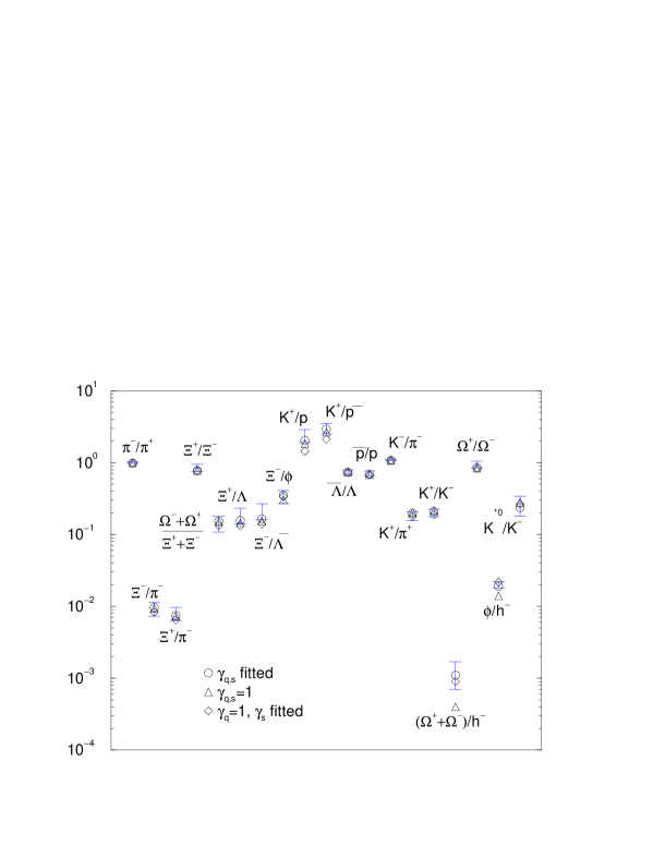
Figure 2: A comparison of 130 GeV Au-Au data and the three different statistical models – all results ‘look good’, even if statistical significance varies considerably, see bottom of table 1.

It is immediately apparent that, in models with chemical non-equilibrium, parameter correlation makes it possible to model some particle ratios over a wide range of any parameter. For instance, Fig. 3 shows that once temperature reaches $\sim 130$ MeV, it is possible to model ratios such as $K/\pi$ and $\Xi/\Omega$ using any temperature within the range. It is only when several similar ratios are fitted together that parameters become disentangled.

Figs 3,4,5 also show that some data points are better at disentangling fit parameters than others. Fig. 3 shows that resonances (here $K^{*}$) are ideal for constraining the freeze-out temperature. If compared to a stable particle whose quark composition is identical, all chemical factors ($\lambda,\gamma$) cancel out independently of equilibrium, so the ratio is a function of temperature and flavor content alone. When the $K^{*}/K$ ratio has been measured to a greater precision, it will be possible to definitely constrain the freeze-out temperature. This could be sufficient to distinguish an equilibrium scenario from one where $\gamma_{q}$ is needed to explain hadronic abundance.

Constraining chemical potentials, in particular to ascertain directly if $\gamma_{q,s}\neq 1$ are present, is more difficult, since these parameters are strongly correlated with temperature. Thus measurement of resonances also fixes this issue, in an indirect way. In addition, as Fig. 5 shows, $\gamma_{s}$ can be constrained by measuring ratios of particles of similar mass, but different strangeness content, such as $\Xi$ and $\Lambda$, while $\gamma_{q}$ (Fig. 4) is sensitive to ratios between baryons and mesons. At the moment, the error bars for these data points are too large to allow disentangling $T$, $\gamma_{q}$ and $\gamma_{s}$.

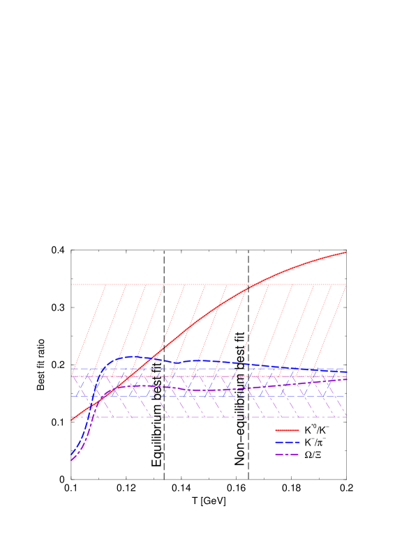
Figure 3: Sensitivity of a measurement of $K^{*0}/K^{-},K^{-}/\pi^{-},\Omega/\Xi^{-}$ on Temperature $T$, other statistical hadronization model parameters have been optimized to best fit the other experimental RHIC-130 data.

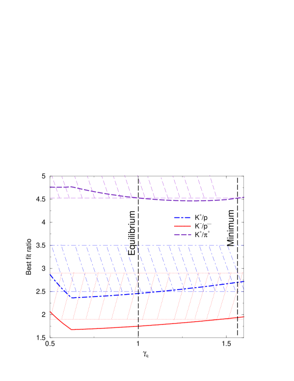
Figure 4: Sensitivity of a measurement of $K^{+}/p,K^{-}/\bar{p}^{-},K^{+}/\pi^{+}$ on the value of $\gamma_{q}$, the chemical light quark pair occupancy parameter, other statistical hadronization model parameters have been optimized to best fit the other experimental RHIC-130 data.

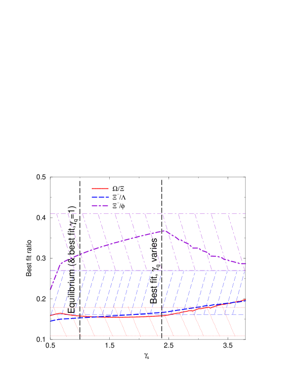
Figure 5: Sensitivity of a measurement of $\Omega/\Xi^{-},\Xi^{-}/\Lambda,\Xi^{-}/\phi$ on the value of $\gamma_{s}$, the chemical strange quark pair occupancy parameter, other statistical hadronization model parameters have been optimized to best fit the other experimental RHIC-130 data.

4 How to SHARE

In the following years, the high-statistics RHIC date, beginning with 200 GeV run will be thoroughly analyzed, leading to better determination of the yields of many stable particles and resonances. As shown in the previous section, these measurements should be sufficient to distinguish between models described above. In addition, SPS and eventually the future GSI facility, as well as higher energy LHC measurements promise an extensive energy scan, allowing a full assessment of the applicability of different statistical models in a wide range of $\sqrt{s}$, as well as the detection of any systematics in the fit parameters.

We have argued that, if the purpose of statistical analysis is to observe an eventual phase transition, any assumptions about chemical equilibration have to be tested against experimental data. We have also argued that statistical hadronization calculations require a very detailed input of the hadronic spectrum, in particular in regard to the uncertainty in degeneracy and decay patter of the higher-lying states [24, 25] as well as experiment-specific weak-decay feed-downs.

To get the correct physics out the experimental data, and to ascertain the physical significance behind the statistical model, these approaches need to be compared with experimental data using a standard procedure. We have proposed an open source general model for: Statistical HAdronization with REsonances (SHARE) [42]. This statistical hadronization package is suitable for comparative analysis of heavy ion collisions in a variety of systems, energy ranges, and equilibrium assumptions. A cross check with SHARE requires that:

1. the resonance decay tree be the same for the different models under consideration, so as all systematic effects in the fit parameters and the quality of the fit deriving from choice of resonance decay are under control,

2. experiment-specific weak decay acceptances should be treated separately for each experimental data-point, to minimize systematic errors on fit parameters deriving from experimental effects,

3. each model’s ability to fit data should be compared in a way that takes into account the different number of degrees of freedom within each model. Statistical significance is a comparison criterion which satisfies this requirement,

4. the fitting program should be able to fit each model’s fit parameter, or constrain it using conservation laws (if applicable),

5. the fitting program should be able to evaluate the fit’s sensitivity to each parameter checking for false minima, etc. and employing $\chi^{2}$ profiles and contours,

6. the fitting program should be able to test the fit’s sensitivity to each data point. This is invaluable both to determine the consistency of the fit, and to detect systematic violations indicating possible novel microscopic formation mechanisms,

7. to better assess the physical soundness of the statistical picture, bulk quantities (total number of negative/positive/neutral particles, entropy, pressure, energy density etc.should also be calculated.

All these features are part of the package SHARE [42]. Moreover we offer three different evaluation of particle multiplicities (SHARE FORTRAN, Mathematica SHARE, and web based SHARE - derived from the FORTRAN version of SHARE). SHARE calculates yields, ratios and bulk quantities in terms of thermodynamic parameters, Fortran version performs fits, and explores parameter sensitivity to data ($\chi^{2}$ profiles, contours etc.). The resonance decay trees, and weak corrections are allowed form and Fortran version requires in the fit the experimental ratios as input.

The reader interested in this field is encouraged to use SHARE in study by means of statistical hadronization models new experimental data. The program is available online, at
http://www.physics.arizona.edu/$\sim$torrieri/SHARE/share.html
http://www.ifj.edu.pl/Dept4/share.html
We hope that this effort will contribute in achieving a better understanding of the applicability and physical significance of the statistical particle production picture.

Acknowledgments

Work supported in part by grants from: the U.S. Department of Energy DE-FG03-95ER40937 and DE-FG02-04ER41318, NATO Science Program PST.CLG.979634. LPTHE, Univ. Paris 6 et 7 is: Unité mixte de Recherche du CNRS, UMR7589. G. Torrieri thanks the organizers of the Krakow school for theoretical physics for the opportunity to present this work, and Charles Gale and SangYong Jeon for helpful and stimulating discussions. We thank Wojtek Broniowski and Wojtek Florkowski for a fruitful collaboration on the SHARE project.

References

- [1] J. Kapusta, B. Muller and J. Rafelski, Quark–Gluon Plasma: Theoretical Foundations An annotated reprint collection, Elsevier, ISBN: 0-444-51110-5, 836 pages, 2003.
- [2] W. Broniowski and W. Florkowski, Phys. Lett. B490, 223 (2000).
- [3] J. Letessier and J. Rafelski, Cambridge Monogr. Part. Phys. Nucl. Phys. Cosmol. 18, 1 (2002).
- [4] R. Hagedorn, Nuovo Cim. Suppl. 3, 147 (1965).
- [5] E. Schnedermann, J. Sollfrank, and U. Heinz, Phys. Rev. C 48, 2462 (1993).
- [6] P. Braun-Munzinger, J. Stachel, J. P. Wessels, and N. Xu, Phys. Lett. B 344, 43 (1995); Phys. Lett. B 365, 1 (1996).
- [7] J. Rafelski, J. Letessier, and A. Tounsi, Acta Phys. Pol. B 27, 1035 (1996).
- [8] T. Csörgő and B. Lörstad, Phys. Rev. C 54, 1390 (1996).
- [9] J. Cleymans, D. Elliott, H. Satz, and R. L. Thews, Z. Phys. 74, 319 (1997).
- [10] J. Rafelski, J. Letessier, and A. Tounsi, Acta Phys. Pol. B 28, 2841 (1997).
- [11] J. Cleymans and K. Redlich, Phys. Rev. Lett. 81, 5284 (1998).
- [12] P. Braun-Munzinger, I. Heppe and J. Stachel, Phys. Lett. B 465, 15 (1999).
- [13] G. D. Yen and M. Gorenstein, Phys. Rev. C 59, 2788 (1999).
- [14] M. Gaździcki and M. Gorenstein, Acta Phys. Pol. B 30, 2705 (1999).
- [15] M. Gaździcki, Nucl. Phys. A 681, 153 (2001).
- [16] F. Becattini, J. Cleymans, A. Keranen, E. Suhonen, and K. Redlich, Phys. Rev. C 64, 024901 (2001).
- [17] F. Becattini, J. Cleymans, A. Keranen, E. Suhonen, and K. Redlich, arXiv:hep-ph/0011322.
- [18] W. Florkowski, W. Broniowski, and M. Michalec, Acta Phys. Pol. B 33, 761 (2002).
- [19] T. Csörgő, Heavy Ion Phys. 15, 1 (2002).
- [20] W. Broniowski, A. Baran, and W. Florkowski, Acta Phys. Pol. B 33, 4235 (2002).
- [21] J. Rafelski, J. Letessier, and A. Tounsi, Acta. Phys. Pol. A 85, 699 (1994). J. Letessier, J. Rafelski and A. Tounsi, Phys. Rev. C 50, 406 (1994); [arXiv:hep-ph/9711346].
- [22] D. Magestro, J. Phys. G 28, 1745 (2002).
- [23] W. Broniowski and W. Florkowski, Phys. Rev. Lett. 87, 272302 (2001).
- [24] K. Hagiwara et al., Particle Data Group Collaboration, Phys. Rev. D 66, 010001 (2002), see also earlier versions, note that the MC identification scheme for most hadrons was last presented in 1996.
- [25] W. Broniowski, W. Florkowski and L. Y. Glozman, arXiv:hep-ph/0407290.
- [26] H. Terazawa, Phys. Rev. D 51, 954 (1995).
- [27] G. J. Gounaris and J. J. Sakurai, Phys. Rev. Lett. 21, 244 (1968).
- [28] P. Koch, B. Muller and J. Rafelski, Phys. Rept. 142, 167 (1986).
- [29] Phys. Lett. B 475, 213 (2000) [arXiv:nucl-th/9911043].
-
[30]
J. Rafelski,
Phys. Lett. B 262, 333 (1991);
J. Letessier, A. Tounsi, U. W. Heinz, J. Sollfrank and J. Rafelski, Phys. Rev. D 51, 3408 (1995) [arXiv:hep-ph/9212210];
F. Becattini, M. Gazdzicki and J. Sollfrank, Eur. Phys. J. C 5, 143 (1998) [arXiv:hep-ph/9710529];
J. Cleymans, B. Kaempfer, P. Steinberg and S. Wheaton, J. Phys. G 30, S595 (2004) [arXiv:hep-ph/0311020]. - [31] J. Rafelski and M. Danos, Phys. Lett. B 97, 279 (1980).
- [32] S. Hamieh, K. Redlich and A. Tounsi, Phys. Lett. B 486, 61 (2000) [arXiv:hep-ph/0006024].
- [33] K. Redlich and A. Tounsi, Eur. Phys. J. C 24, 589 (2002) [arXiv:hep-ph/0111261].
- [34] J. Rafelski and J. Letessier, J. Phys. G 28, 1819 (2002) [arXiv:hep-ph/0112151].
- [35] F. Antinori et al. [NA57 Collaboration], Phys. Lett. B 595, 68 (2004) [arXiv:nucl-ex/0403022].
- [36] G. E. Bruno [NA57 Collaboration], J. Phys. G 30, S717 (2004) [arXiv:nucl-ex/0403036];
-
[37]
T. Virgili et al. [NA57 Collaboration],
“Recent results from NA57 on strangeness production in p A and Pb Pb
collisions at 40-A-GeV/c and 158-A-GeV/c,”
arXiv:hep-ex/0405052;
D. Elia et al. [NA57 Collaboration], “Strange particle production in 158 and 40 GeV/ Pb-Pb and p-Be collisions,” Contribution to the proceedings of the ”Hot Quarks 2004” Conference, July 18-24 2004, New Mexico, USA, submitted to Journal of Physics G, arXiv:nucl-ex/0410034. - [38] G. Torrieri and J. Rafelski, arXiv:hep-ph/0409160.
- [39] J. Letessier and J. Rafelski, Int. J. Mod. Phys. E 9, 107 (2000) [arXiv:nucl-th/0003014].
- [40] M. Kaneta and N. Xu, arXiv:nucl-th/0405068.
- [41] F. Becattini, M. Gazdzicki, A. Keranen, J. Manninen and R. Stock, Phys. Rev. C 69, 024905 (2004) [arXiv:hep-ph/0310049].
- [42] G. Torrieri, W. Broniowski, W. Florkowski, J. Letessier and J. Rafelski, arXiv:nucl-th/0404083.