STUDY OF DISSIPATIVE DYNAMICS IN FISSION OF HOT
NUCLEI USING
LANGEVIN EQUATION
THESIS SUBMITTED TO
JADAVPUR UNIVERSITY
FOR THE DEGREE OF
DOCTOR OF PHILOSOPHY IN SCIENCE
(PHYSICS)
by
GARGI CHAUDHURI
Variable Energy Cyclotron Centre
Department of Atomic Energy
1/AF Bidhannagar, Kolkata-700 064
July 2004
To the memory of my uncle
Bimal kumar Chaudhuri
CERTIFICATE FROM THE SUPERVISOR
This is to certify that the thesis entitled “ Study of dissipative dynamics in fission of hot nuclei using Langevin equation” submitted by Smt. Gargi Chaudhuri who got her name registered on 16.02.2001 for the award of Ph.D.(Science) degree of Jadavpur University, is absolutely based upon her own work under the supervision of Dr. Santanu Pal, Variable Energy Cyclotron Centre, and that neither this thesis nor any part of it has been submitted for any degree/diploma or any other academic award anywhere before.
(Signature of the Supervisor & date with official seal)
Acknowledgements
It gives me great pleasure to acknowledge my indebtness to Dr. Santanu Pal, my thesis supervisor, for his invaluable guidance and encouragement ever since I took up theoretical physics as my career. He has shown me the path and lighted it for me through his useful suggestions, thorough discussions and fruitful criticism, thus helping me to contribute a tiny bit to this vast sea of nuclear physics. The completion of this thesis owes very much to his support and his keen interest and involvement in the work.
I take this opportunity to express my sincere gratitude to Prof. Bikash Sinha, Director, Variable Energy Cyclotron Centre(VECC) and Dr. Jadu Nath De, former Head, Physics Group, VECC, for being instrumental in my joining the theoretical physics division of this centre. I owe a lot to Dr. Jadu Nath De for being extremely caring and motivating throughout the period of this work. I am grateful to our Director as well to Dr. Dinesh Kumar Srivastava, Head, Physics Group, VECC, for providing the congenial atmosphere and full fledged facility which helped me immensely during my work. I remember with gratitude the valuable discussions with Dr. Asish Kumar Dhara which inspired me to probe deeper into the subject.
I remember with deep respect my teachers of Jadavpur University as well as Indian Institute of Science, Bangalore, who have inspired me to enjoy Physics and share the mystery of nature with all other researchers like me. That I am still continuing with Physics owes a great deal to all of them.
I am thankful to the Computer Division of VECC for providing advanced computing facilities which helped a lot in successful completion of my work. I also thank the members of Physics Group office as well as the Director’s office for their cooperation at various stages. Last but not the least, I should thank all the members of VECC library for providing the necessary help throughout.
I remember with great pleasure all my friends in VECC, both past and present, whose company and friendship have refreshed and energized me during my research tenure. I would like to make special mention of Dr. Ranjana Goswami, Mr. Partha Ghosh, Dr. Tapas Sil, and Dr. Debasish Bhowmick all of whom shared with me my moments of joy and sorrow. I convey my sincere thanks to all my colleagues in VECC who have made my thesis tenure memorable.
At this juncture, I am very much reminded of Somshubhro who has been my most intimate friend ever since I chose Physics as my career in B.Sc. My interest to continue in Physics owes a lot to the discussions we had during our university days to clear the doubts regarding different aspects of this great subject. I remember with pride his support and concern for me both as my friend and as my husband and his constant advices to be always hardworking and sincere in my effort. I remember with deep affection the support and company of my brother Balarko and the technical suggestions given by him while writing this thesis.
I fondly remember the cheerful face of my little daughter Jhelum who have been my constant source of energy and delight. The completion of this thesis have somewhat deprived her of the due attention and time for which I feel guilty. I am really at a loss of words to express my obligation to my parents who have supported me all through, and have taken up the greater chunk of my responsibilities allowing me enough opportunity to proceed smoothly with my work. This thesis owes most to them. At this moment I very much remember with gratitude that both my father and my husband always insisted on giving my research work the first priority and encouraged me to produce my best.
Today on the verge of climbing a vital step of my career, I gratefully remember the blessings and affection of all my well wishers (specially my aunt) since my childhood which have contributed in shaping up my life and my career. I also gratefully acknowledge the encouraging words of my parent-in-laws in my journey towards the goal.
On completion of this thesis, when my hope gets realized, I could visualize the extreme delight of my departed uncle who cherished the dream more than me and would have been the happiest person on this little achievement. I very much remember his unlimited love, his deep concern, his constant encouragement throughout my academic career and the moral boosts I received from him on every little success that I achieved. I consider myself very fortunate to have him as my greatest well wisher. I feel extremely sad that he is no more by my side to share my moments of joy. I cannot put this thesis in his hands today; I can only dedicate it to his sacred memory.
PREFACE
The advent of high energy heavy ion beams in various energy ranges has led to the discovery of a number of significant nuclear phenomena. The fission of highly excited compound nuclei formed in heavy ion induced fusion reactions has emerged as a topic of considerable interest in the recent years. Multiplicity measurements of light particles and photons strongly suggest that fission is a much slower process for hot nuclei than that determined from the statistical model of Bohr and Wheeler based on phase space arguments. This led to the introduction of dynamical effects, specially the concept of nuclear friction in the description of fission of hot nuclei. Dissipative dynamical models based on the Langevin equation were developed and were applied successfully for fission dynamics of highly excited heavy nuclei. However, Wall Friction(WF), the standard version of nuclear friction when incorporated in the Langevin dynamical model was not able to reproduce simultaneously experimental data for both prescission neutron multiplicity () and fission probability (). Consequently, an empirical reduction in the strength of the wall friction was found necessary to reproduce the experimental numbers by many workers. Interestingly, a modification of the wall friction was proposed recently where the reduction was achieved microscopically. This modified version is known as the chaos weighted wall friction(CWWF) which takes into account non-integrability of single particle motion. The work in my thesis aims at using this strongly shape dependent version of friction (CWWF) in the Langevin dynamical model coupled with particle and gamma evaporation in order to verify to what extent it can account for the experimental data of fission of hot nuclei. The present endeavour is an effort to obtain a clear physical picture of nuclear dissipation which in turn will help in solving many open problems related to collective motion, and in particular, nuclear fission. An important application of current interest could be the theoretical prediction of survival probability of superheavy elements against fission which depends sensitively on nuclear dissipation on the fission path.
Outline of the thesis:
The work to be presented in this thesis is divided into seven
chapters and seven appendices. Chapter 1 gives an overview of the
subject, where the relevant literature is reviewed briefly. In
Chapter 2 our model for Langevin dynamics of nuclear fission will
be described in details. The origin of the different inputs used
in our calculation, namely, potential, inertia and level density
parameter will be discussed. The chaos weighted wall friction
which is used for nuclear dissipation in the dynamics and will be
tested for the first time will be described elaborately in this
chapter. Chapter 3 contains the procedure of solving the Langevin
equation for strongly shape dependent friction in order to
calculate fission width which are subsequently utilized in further
calculations. The fission widths are calculated using both the
wall friction and the chaos weighted wall friction. In Chapter 4,
the different steps of the combined dynamical and statistical
model which couples particle and evaporation with
Langevin dynamics, is described. The excitation functions of the
prescission neutron multiplicity and the fission probability
calculated from the model using both the versions of the friction
are compared with the experimental data for a number of nuclei in
this chapter. Chapter 5 is devoted to the calculation of the
evaporation residue cross section excitation function as a probe
for nuclear friction which is compared with experimental data.
Chapter 6 discusses in details the effects of transients in
nuclear fission on prescission neutron multiplicity. Chapter 7
contains the thesis summary, conclusions and future directions of
our work. Some details of the formulation and the computation are
given in the different appendices. The cumulative references for
all the chapters are given at the end.
Based on the work presented in this thesis, following papers have been published in refereed international journals. The listings at http://arXiv.org are given at the end of each reference.
List of Publications:
-
1.
Fission widths of hot nuclei from Langevin dynamics,
Gargi Chaudhuri and Santanu Pal, Phys.Rev. C63 (2001) 064603; nucl-th/0101037 -
2.
Prescission neutron multiplicity and fission probability from Langevin dynamics of nuclear fission,
Gargi Chaudhuri and Santanu Pal, Phys.Rev. C65 (2002) 054612; nucl-th/0105010 -
3.
Effect of transients in nuclear fission on multiplicity of prescission neutrons,
Gargi Chaudhuri and Santanu Pal, Eur.Phys.J. A14 (2002) 287-294; nucl-th/0204052 -
4.
Evaporation residue cross-sections as a probe for nuclear dissipation in the fission channel of a hot rotating nucleus,
Gargi Chaudhuri and Santanu Pal, Eur.Phys.J. A18 (2003) 9-15; nucl-th/0306003
Gargi Chaudhuri
Variable Energy Cyclotron Centre,
1/AF, Bidhannagar, Kolkata, India.
Chapter 1 Introduction
The study of large scale nuclear dynamics (e.g. deep inelastic collisions and fission) initiated by energetic heavy ion beams above the Coulomb barrier is an active area of research in nuclear physics and presents a number of theoretical challenges. In particular, one of the exciting aspects in such studies is that in these energetic nuclear reactions, concepts of non-equilibrium statistical physics, such as dissipation or thermalization, are extended to small and dense Fermion systems. The energy scale under consideration here ranges from that above the Coulomb barrier and extends up to the Fermi energy domain( 30 MeV/nucleon). The availability of heavy-ion beams in various energy ranges and the emergence of exclusive measurements in different experiments (which provide more insight into the nuclear dynamics than the inclusive experiments) motivated the development of theoretical approaches such as transport theories and the time dependent Hartee-Fock(TDHF) theory. In particular, the transport theories[1, 2] were developed using the general framework of nonequilibrium statistical physics, the kinetic theory and the stochastic methods. In such descriptions dissipation, i.e., the irreversible flow of energy between the collective and intrinsic degrees of freedom of the system and the associated fluctuations play very important role. An estimate of the nuclear dissipation or friction was first made from the analysis of deep inelastic collision and heavy ion induced fusion experimental data with classical trajectory models[3, 4]. However the results turned out to be widely varying even by orders of magnitude. The advent of exclusive measurements and sophisticated experimental techniques as well as the development of improved theoretical models contributed in narrowing down the range of magnitude of nuclear friction to a great extent. A comparison of the experimental results with the phenomenological Langevin or Fokker-Planck models has allowed to extract the key parameters entering these description, namely the nuclear friction. On the other hand, the microscopic derivation of the nuclear friction coefficient has attracted a large amount of theoretical effort. Over the years, different microscopic as well as phenomenological attempts have been made to derive the nuclear friction coefficient but any unambiguous prescription for nuclear friction is yet to be achieved. In this thesis, we shall be concerned with a detailed study of the fission dynamics of highly excited nuclei formed in heavy-ion collisions using a theoretical model of nuclear dissipation(a modified version of the wall friction). Our main aim in this work is to test this theoretical model as a candidate for nuclear friction without any tunable parameter. Such a nuclear friction has immense applicability in predicting survival probability of superheavy nuclei against nuclear fission and production cross section of fission fragments in ISOL-type radioactive ion beam facilities.
1.1 Overview
1.1.1 General
In order to present an overview of the advances of the many body aspects of nuclear dynamics, it is illuminating to begin with one of the most fundamental contributions to this field credited to Niels Bohr, whose work had a profound impact on the post-1930s development of nuclear physics. The pioneering contribution to this field is the “compound nucleus theory” of Bohr which has a fascinating appeal in many aspects of nuclear dynamics. The basic idea of the compound nucleus model is a strong and intimate coupling of all the nucleons with each other. This subsequently led to the development of the nuclear liquid drop model by Bohr and Kalckar[5]. It was this model which enabled Meitner and Frisch[6] to explain why a nucleus may undergo fission, and this led Bohr and Wheeler[7] to develop their celebrated formula for a first quantitative description of the decay rate of nuclear fission. This work also laid the foundation for the concept of nuclear collective motion. The standard analysis of induced nuclear fission is based on the Bohr-Wheeler formula for the fission width which depends on the ratio of the phase spaces available at the saddle point to that at the ground state and is given by the following expression.
| (1.1) |
where is the excitation energy, is the height of the fission barrier, is the kinetic energy, and is the density of levels of the compound nucleus at the saddle point which arises from excitations of the intrinsic degrees of freedom only and denote the level densities of the fissioning nucleus at the ground state. A simplified expression is obtained with the Fermi gas model for the level densities which is given by , the constant temperature approximation and the condition
| (1.2) |
where is the usual level density parameter. It yields the fission width as a function of the fission barrier height and the nuclear temperature T. This description of nuclear fission does not invoke any dynamical features and hence is independent of the nuclear friction. It is however interesting to note that it is mentioned in the addendum of Bohr’s paper[5] that “non-viscous fluid can hardly be maintained in view of the close coupling between the motions of the individual nuclear particles.” Kramers[8] took up this point and derived a formula for the fission decay rate in which a correction factor(K) appeared to the Bohr-Wheeler expression, which was governed by nuclear friction. Kramers formula for fission width () is related to that of Bohr-Wheeler () by the factor , where is proportional to the nuclear friction coefficient . Kramers pictured the collective motion as a transport process in collective phase space. He dealt with the general problem of Brownian motion in a heat bath in the presence of a potential barrier. The importance of Kramers idea was realized much later in nuclear physics with the advent of heavy ion accelerators with which nuclear systems could be excited to much higher energies and it was thus realized that the energy stored in the collective motion can be dissipated.
Different microscopic theories were developed to describe nuclear collective motion. This began in the early fifties with the unified model of Bohr and Mottelson [9]. Small amplitude collective motion like the normal vibration modes of a nucleus were explained by the random phase approximation(RPA)[10]. However, the RPA is typically a small amplitude approximation, and cannot describe collective processes during which nuclear wave function undergoes important alterations, such as fission, fusion, heavy ion reactions etc. Microscopic theories for large amplitude motion of many body fermion systems are usually based on a mean field description known as time dependent Hartee-Fock method(TDHF) developed in the 1970s, and its variants like ATDHF [10]. The TDHF equation is a nonlinear equation for the one-body density matrix and a first-order differential equation in time, which in its simplest form reads like
| (1.3) |
with . is the kinetic energy, and is the self consistent mean field which depends on the density of the nucleus. It was realized that as the excitation energies become higher and is around the regime of Fermi energy/nucleon, the nucleon-nucleon correlations become dominant over the effects of the averaged forces and it would be thus necessary to look beyond mean field description. Application of TDHF requires a large mean free path and hence is a good approximation for the low energy heavy ion collisions. However, at high collision energies, the mean free path is strongly reduced due to the large excitation energies involved in the process. Thus the inclusion of residual two-body collisions in a self consistent mean-field theory (generalized or extended TDHF) is a natural step of a more realistic description of heavy-ion collisions at high excitation energies. However, because of numerical difficulties, realistic applications of these approaches seem to be difficult even with the fastest available computers. This has been tried in various versions but it had soon become clear that all one is able to do numerically is to solve such equations in a semi-classical limit, e.g., in the version of the Boltzman-Uehling-Uhlenbeck(BUU) or Landau-Vlasov equation[11]. The BUU equation is as follows
| (1.4) | |||||
where the right hand side is the collision integral including the Pauli blocking and when it is set equal to zero, one obtains the Vlasov equation.
The macroscopic variables behind TDHF are the ones which relate to matrix elements of the one-body density operator. A much simpler version is given if one parameterizes the time evolution of the mean field by time dependent shapes and provided it is possible to complement such a description with the dynamics of a conjugate momentum, one may view this motion as a transport process in collective phase space. This gave rise to the revival of the theoretical studies based on the original works of Kramers who viewed the collective dynamics on similar lines. There have been (a) applications of linear response theory to formulate a theoretical description appropriate for heavy-ion collisions by Hofmann and Siemens[12, 13], (b) the applications of the methods of spectral distributions or the random matrix model by the groups of Nörenberg [14] and Weidenmüller[1, 14, 15] and (c) the suggestion of Norenberg to model relative motion of two heavy ions by way of a “dissipative, diabatic dynamics(DDD)” [2]. The linear response theory aims at describing large-scale collective motion on the basis of a locally harmonic approximation. This approximation is exploited to define propagators and to derive equations for their dynamics in small areas of phase space and over time lapses which are small on a macroscopic scale. In the work of Weidenmüller et al.[15], the statistical properties of matrix elements which couple the collective degrees of nuclear motion with the intrinsic degrees of freedom, are evaluated in an adiabatic approximation. A random-matrix model is used for the residual interaction. The basic idea of DDD[16, 17] is that the energy dissipation in slow collective nuclear motion is viewed as a combined effect of a diabatic production of particle-hole excitations, leading to a conservative storage of collective energy, and a subsequent equilibration due to residual two-body collisions. The effective equation of motion for the collective degree of freedom contains a time retardation in the dissipative term and allows for a simultaneous description of two different attitudes of nuclear matter. The elastic response of heavy nuclei for ‘fast’ collective motion switches over to pure friction for very ‘slow’ collective motion. A first application of the diabatic dynamical approach is made for the quadrupole motion within a diabatic deformed harmonic oscillator basis.
The concept of friction and the associated statistical fluctuations play an important role in many areas of physics, chemistry and biology, when one is dealing with transport processes. The equations which are usually applied are master equations, Fokker-Planck equations and Langevin equations. The books of Risken [18], Van Kampen[19], and the article of Hanggi et al.[20] provide complete mathematical background of the subject. With the discovery of deep-inelastic processes in heavy-ion collisions, the concept of friction was introduced in the description of complex nuclear reactions, where it was impossible to follow all involved degrees of freedom explicitly. First, models with classical trajectories which are determined by conservative and frictional forces have been developed[4]. Then, Norenberg [21] introduced a Fokker-Planck equation for the description of charge transfer as a diffusive process in deep-inelastic heavy-ion collisions. Subsequently, multi-dimensional Fokker-Planck equations were applied by many authors in order to describe deep-inelastic differential cross sections with respect to the scattering angle, energy loss, and to mass and charge transfer variables.
It has always been a challenge to extend Kramers’ result of the decay of a metastable system to the quantal regime. It was only in the 80’s that one began to understand how to incorporate quantum effects and among the vast literature available on “dissipative tunneling” one may refer to [20, 22, 23]. Common to all these approaches is the application of the technique of path integrals for imaginary time propagation. For nuclear fission and nuclear multifragmentation, a formulation with real time propagation is much more appropriate. This has been achieved by a suitable application of linear response theory. The transport equation obtained is similar in structure to that of Kramers’, with only the diffusive terms being modified to take account of the quantum effects[24]. The modification of Kramers’ equation using quantal diffusion coefficients is also studied in Ref. [25]. In Ref. [26], the decay of a metastable system is described by extending Kramers’ method to the quantal regime. It is seen that the quantum corrections to the decay rate would lead to an increase of the later [27]. This effect is significant for temperatures of the order of 1 MeV or less.
1.1.2 Nuclear Fission
Nuclear fission is one of the earliest and most thoroughly studied of all nuclear phenomena. Fission is the most prominent and classic example of ‘slow’ large-scale collective motion in nuclear physics. The standard statistical model of Bohr and Wheeler [7] was sufficient for a long time to describe the observed effects of nuclear fission till the availability of high energy heavy-ion beams. A spate of experimental data from heavy-ion induced reaction studies, carried out in the last two decades have resulted in the interesting observation of unexpectedly large pre-scission yields of charged particles [28], neutrons [29], and giant dipole resonance(GDR) decay rays [30] from the compound system before fission. The standard statistical model was found to underestimate the prescission yields of particles and -rays, the discrepancy being large at excitation energies greater than 50 MeV. The underestimation of prescission particles at high excitation energies by the statistical model led one to think that sufficient time is not available for the particles to evaporate prior to fission. In other words, the fission width calculated on the basis of phase space arguments is overestimated in statistical model at high excitation energies. At lower excitation energies the standard statistical model calculations hold good because in this energy regime, the particle multiplicity has negligible dependence on the fission width and hence the simplified arguments used in statistical model was sufficient to reproduce the particle multiplicities. However, with the increase in the excitation energies, fission width increases and becomes comparable to the particle emission widths and the dependence of the particle multiplicities on fission width becomes significant. This realization motivated more rigorous calculation of the fission width invoking dynamical effects at higher excitation energies and led one to look beyond the standard statistical model. The experimental data revealed that fission of hot nuclei is a slower process than that predicted by the statistical model. The need for a slowing down mechanism naturally suggests one to consider the effects of nuclear friction on fission lifetime and this inspired the use of a transport description of fission since it includes the dynamical features not contained in the statistical model. This gave rise to the revival of the theoretical studies based on the original works of Kramers who considered induced nuclear fission as a transport process of the fission degree of freedom over the fission barrier as a consequence of thermal fluctuations. Dissipative dynamical models for fission of hot nuclei based on the transport theory were subsequently developed.
1.2 Dissipative dynamical model of nuclear fission
1.2.1 Introduction
The goal of any transport theory is to reduce the description of the time evolution of a complex system to that of a small subset of its degrees of freedom. The dynamics of the residual set is not explicitly considered though their effect is taken into account in some average sense. Often the first class of variables is referred to as the collective or “macroscopic” ones, whereas the rest of the degrees of freedom is referred to as the “intrinsic” system. The notion macroscopic indicates that in many cases these variables are chosen to represent quantities whose dynamics can be visualized as a transport of matter, total charge etc. A macroscopic description of fission dynamics is based on the idea that the gross features of the fissioning nucleus can be described in terms of a small number of variables called the collective variables or the collective degrees of freedom. At nuclear excitations which give rise to temperatures up to a few MeV , the dominant collective modes relevant for nuclear fission are expected to be those involving changes in the nuclear shape, and the coordinates of the nuclear surface itself provide a natural set of collective variables. In the transport theory which is also referred to as the dissipative dynamical model, the dynamics associated with the fission degree of freedom(collective motion) with a large inertial mass is considered to be similar to that of a massive Brownian particle floating in a viscous heat bath under the action of a potential field. The rest of the nuclear system comprising of a large number of intrinsic degrees of freedom (assumed to be in thermal equilibrium) is identified with the heat bath. It is also assumed that the impact of Brownian particle dynamics on the heat bath is insignificant. It is of great importance, however, to understand how the heat bath influences the dynamical macroscopic object. In fact, the introduction of the heat bath makes the dynamics of the Brownian particle irreversible and will exhibit fluctuations in observable quantities. Fluctuations arise in the theoretical description, because attention is focussed entirely on a few degrees of freedom (the collective variables), and the loss of information caused by disregarding the many other degrees of freedom manifests as sizeable fluctuations in physical observables. In most cases the inertial mass associated with the collective degree of freedom is large enough so that its dynamics is governed entirely by the laws of classical physics. This separation of the whole system into a Brownian particle and a heat bath relies on the basic assumption that the equilibration time of the intrinsic degrees of freedom() is much shorter than the typical time scale of collective motions(), i.e, the time over which the collective variables change significantly. The separation of these two time scales allows the decomposition of the Hamiltonian into a collective part(describing the shape degrees of freedom) and a intrinsic part (describing the intrinsic degrees of freedom). Moreover, if one assumes that the intrinsic motion loses memory very quickly, one can easily derive transport equations for the collective degrees of freedom. If is the time it takes the entire system to return to a point very close to its original position in phase space (Poincar recurrence time) then it should be much greater than the time scale for collective motion so that the collective dynamics is irreversible. Thus the time scales governing the behavior of an equilibrating system must obey the following inequalities for a transport description to be viable.
| (1.5) |
The domain of applicability of transport theories has been extensively discussed in the case of deep inelastic heavy-ion reactions in Ref. [1]. Later it was found that transport theories can also be applied for describing competitive decay of composite nuclear systems [31]. The crucial parameters in a diffusion model for fission are the nuclear friction , which gives the strength of the coupling between the fission and the intrinsic degrees freedom, and the diffusion constant , related to each other by the Einstein relation. A diffusion model is applicable to fission when the internal equilibration time of the heat bath is small compared to the characteristic time of the diffusion process itself(related to ), and to (=) and (=), where ()are the fission (neutron) widths at the excitation energies under consideration. On the basis of microscopic considerations, simple estimates of these time scales(leading to sec) suggest a diffusion model is applicable for sec-1 [32] ( being the mass of the Brownian particle), and for excitation energies of 100 MeV or more. We shall assume that the transport(diffusion) equation will be applicable to nuclear fission at high excitation energies in the dissipative dynamical model.
The description of the intrinsic modes of excitation in terms of a heat bath has two consequences. First, energy flows irreversibly from the collective motion into the intrinsic excitation and manifests as a friction force in the collective dynamics. Second, the fact that the dynamics of the intrinsic degrees of freedom, collectively represented by the temperature T, are uncorrelated gives rise to random features in the coupling between the heat bath and the collective motion. As a consequence energy is exchanged randomly in both directions in a fine time scale, though the net flow is into the heat bath over a larger time scale. Thus, the time development of the collective variable has a random character. This is analogous to that of a Brownian particle which collides with gas molecules having a Maxwellian velocity distribution. The Brownian particle undergoes a random walk and is slowed down but on a staggering path. The motion of a Brownian particle in an external force field which essentially is the model of fission dynamics considered here, can be described by two alternative but equivalent mathematical formulations, which will be briefly described in the following subsections.
1.2.2 Fokker-Planck equation
The Fokker-Planck equation and the Langevin equation are the two equivalent descriptions of a Brownian particle in a heat bath. The Fokker-Planck equation can be derived starting from the Langevin equation[33]. One begins with the Liouville equation which describes the conservation of probability, i.e., with the continuity equation for probability,
| (1.6) |
where is the distribution function in momentum space. The Langevin equation describing the motion of a Brownian particle of mass (to be described in detail in the next subsection) in the presence of a potential and friction coefficient reads as follows
| (1.7) |
Substituting for from Eq. 1.7 and integrating Eq. 1.6 between and , ( is much larger than the time scale of the random force ) leads to
| (1.8) |
where
| (1.9) |
Taking an average over all possible realizations of the random force and using the properties of (to be discussed in the next subsection), in the limit , it can be shown that
| (1.10) |
where is the mean square strength of the random force. This equation is known as the Fokker-Planck equation or the Kramers equation. The fact that it is possible to derive the Fokker-Planck equation from the Langevin equation (using the continuity equation or the master equation) clarifies the relation between the two equations and establishes their equivalence.
The Fokker-Planck equation is a probabilistic dynamical description and it deals with the time-evolution of the distribution function of the Brownian particle. The probability distribution f(r,p,t) for finding the particle at a point(r,p) in classical phase space is obtained by solving the above Fokker-Planck equation. Kramers(1940) applied it to the decay rate of nuclear fission. He obtained the equilibrium solution of the above equation and derived the quasi stationary fission width from it which is given by the following expression.
| (1.11) |
Here and are the oscillator frequencies of the parabola osculating the nuclear potential in the first minimum and at the saddle respectively. In the limit of small , reduces to the transition state expression given by
| (1.12) |
The Kramers width is related to the Bohr-Wheeler width (Eq. 1.2) through the Kramers factor (also called reduction factor) which is given by . In Eq. 1.12, is the Bohr-Wheeler width corrected for the presence of collective vibrations[34] in the potential pocket not taken into account in the density of levels in Eq. 1.1 (refer section 1.1.1). The Kramers factor depends on the nuclear friction coefficient and is interpreted as a restriction in phase space around saddle point due to friction. It is thus remarkable that the importance of friction in nuclear dynamics was anticipated by Niels Bohr in 1939, and H. A. Kramers correctly predicted a reduction of fission width which was experimentally confirmed after about 50 years. Between 1940 and the beginning of the 80s Kramers approach did not attract much attention in the context of nuclear fission. This happened because the simple Bohr-Wheeler formula worked well, at least within the uncertainties of the fission barrier height and of the level density parameter. Forty years later, in the eighties, Weidenmuller and his group [35] followed the line of approach of Kramers and adopted the diffusion model to investigate how the quasistationary flow over the fission barrier is attained. Their study was motivated by the experimental findings [36] which seemed inconsistent with the Bohr-Wheeler prediction in showing an excess of evaporated neutrons. They succeeded in getting the time dependent solution of the two dimensional Fokker-Planck equation after making a number of simplifying assumptions and obtained the time dependent fission width by calculating the probability current through the saddle point. Their work first showed that for finite values of the friction coefficient , there is a time which elapses between the start of the induced fission process and the attainment of the stationarity condition. This time depends on and during this time fission is suppressed. The larger the value of , more will be the time for evaporation and more strongly will particle and gamma evaporation compete with the fission process. Their study first established the importance of ‘transients’, i.e., those processes which occur before the quasistaionary flow over the barrier is attained. They showed that the fission probability is modified compared to the Bohr-Wheeler formula in two ways: (i) suffers an overall reduction in the stationary fission rate due to friction (reduction factor K of Kramers) (ii) the inclusion of transients reduces further, particularly at higher excitation energies. Both these effects will significantly increase the neutron emission as demanded by the experimental data. It was also shown that the entire fission process becomes a transient when there is no fission barrier [37]. The detailed study of transients in nuclear fission were considered in a series of publications. We shall discuss our own contribution to this topic in chapter 6. Dynamical studies of induced fission with the Fokker-Planck or Kramers equations have also been studied by other groups[38, 39] investigating the reduction of the Bohr-Wheeler width by the Kramers factor as well as the existence of the transient time. These findings stimulated refined measurements of the multiplicities of neutron, light charged particles and photons[29, 40]. Theoretical developments were made for a proper description of the competitive decays of particle evaporation and fission[39, 41, 42], an effect which becomes especially important when one considers the fission of hot nuclei. Multi-dimensional Fokker-Planck equations were subsequently applied to the description of nuclear fission[43].
Analytic solutions of the Fokker-Planck equations were initially restricted to the use of the quasi-linear method, in which the driving terms are expanded to the lowest order and only the first and second moments of the Fokker-Planck equation together with a Gaussian ansatz are used to calculate the distribution function at large times, from which the cross sections can be obtained. However it turns out that in many cases the Gaussian ansatz is not a good approximation. The multi-dimensional Fokker-Planck equations for deep-inelastic collisions and induced fission can be solved numerically with grid methods which is an exact procedure but turns out to be extremely difficult even with present day computers. Modelling the same problem in terms of the equivalent Langevin equations, and solving these equations by Monte-Carlo sampling, is a more practicable way for obtaining more accurate solutions than with the Gaussian ansatz. Suggestions were made to apply Langevin equation in nuclear physics in Refs. [44, 45]. The first calculations using Langevin equation were performed later, for deep-inelastic procesess by Barbosa et al. [46], for fission by Abe et al. [33] and for fusion by Fröbrich[47]. Since then a large volume of work have been reported , which have applied Langevin equation with the aim to describe data for deep-inelastic heavy-ion collisions, fusion, and heavy-ion induced fission.
1.2.3 Langevin equation
Langevin approach which is an alternative description of the Brownian motion was first proposed by Y. Abe [33] as a phenomenological framework to describe nuclear fission dynamics. The Fokker-Planck equation deals with the time evolution of the distribution function(in classical phase space) of the Brownian particle while the Langevin equation deals directly with the time evolution of the Brownian particle and hence is much more intuitive. The two approaches describe different aspect of the dynamics but they are equivalent with respect to their physical content. The motion of a Brownian particle under the action of a external force field as given by the one-dimensional Langevin equation (1.7) can be written as follows,
| (1.13) |
where is the external force and is given by
| (1.14) |
The coupling of the collective motion with the heat bath is described by . It has two parts; a slowly varying part which describes the average effect of heat bath on the particle and is called the friction force (), and the rapidly fluctuating part which has no precise functional dependence on t. Since it depends on the instantaneous effects of collisions of the Brownian particle with the molecules of the heat bath, is a random(stochastic) force with its mean value zero and with a specific probability distribution. It is further assumed[33] that has an infinitely short time correlation, i.e. it describes a Markovian process. Therefore is completely characterized by the following moments,
| (1.15) |
where is the diffusion coefficient and is related to the friction coefficient (to be described later). It should be noted that Langevin equation is different from ordinary differential equations as it contains a stochastic term R(t). In order to calculate physical quantities such as mean values of observables from such a stochastic equation, one has to deal with a sufficiently large ensemble of trajectories for a true realization of the stochastic force. The physical description of Brownian motion is therefore contained in a large number of stochastic trajectories rather than in a single trajectory, as would be the case for the solution of a deterministic equation of motion. The Kramers equation or the Fokker-Planck equation is a partial differential equation which can be solved analytically under simplifying assumptions whereas the Langevin equation is a stochastic differential equation and therefore not amenable to analytic treatment. This is possibly the reason why the Langevin approach was not used in nuclear applications for a long time, while the Fokker-Planck equation was preferred for applications in heavy-ion collisions, especially for the deep-inelastic processes. Further, the Fokker-Planck equation or the Langevin equation are to be solved numerically for practical applications to nuclear collective motions where more than one degree of freedom are involved and the transport coefficients(friction, inertia) are coordinate dependent. Numerically, the Langevin equation is more straightforward to handle for a number of reasons. Firstly, it is easier to accommodate more degrees of freedom in this ordinary differential equation. On the other hand, the Fokker-Planck equation is a partial differential equation and adding more degrees of freedom generates a multidimensional partial differential equation, the solution of which is very time consuming even with modern supercomputers. The multiple reduplication of the trajectory calculation(Langevin approach) is the price one has to pay to avoid solving a partial differential equation in many degrees of freedom. Secondly, the solution of the Langevin equations by Monte-Carlo sampling of trajectories is numerically more stable than the approximate methods available for a direct solution of Fokker-Planck equation[48]. Moreover, the Langevin equation can be extended to include non-Markovian processes as well [48]. It may also be mentioned that there is a quantal version of the Langevin equation based on which a full-fledged transport theory has been formulated in [49] within a quasi-classical approach. By virtue of its intuitiveness, generality, and other practical advantages, Langevin approach is preferred to that of Fokker-Planck and is mostly followed in the recent years.
Both the friction coefficient and the random force arise due to coupling of the collective dynamics with the intrinsic motion of the system. Since they have the same microscopic origin, they are expected to be correlated. In fact in his famous analysis of Brownian motion, Einstein showed in 1905 that the friction coefficient and the diffusion constant (related to by Eq. 1.15) are related to each other. This is intuitively understandable since both of these constants describe different aspects of the same physical process - the exchange of momentum and energy between the collective variable and the heat bath. The argument is universal and applies as well to nuclear systems. It can be shown[48] that there is a relation between them called the ‘fluctuation-dissipation theorem’ which reads as follows
| (1.16) |
where is the temperature of the heat bath. This relation is also supported from a phenomenological analysis. As time approaches infinity, the Brownian particle is expected to be in equilibrium with the heat bath and the average kinetic energy (for one dimensional motion) becomes equal to ( is in units of energy). Using the Langevin equation (1.13) for a free Brownian particle ( = 0) and using the properties of the random force given by Eq. (1.15), the average kinetic energy of the Brownian particle is calculated as follows
| (1.17) |
As , one gets , which yields . Substituting in Eq. (1.15), one finally gets
| (1.18) |
The above relation connects the mean square strength of the stochastic force with the friction coefficient. This fluctuation-dissipation theorem points out the cause-effect relationship between the stochastic and dissipative component of the dynamics. It also implies that any dissipation is always associated with fluctuations and vice versa.
In the dissipative dynamical model of nuclear fission discussed previously, it is assumed that the fission of hot nuclei involves two distinct time scales; one being associated with the slow motion of the fission degrees of freedom and the other with the rapid motion of the intrinsic degrees of freedom. The time evolution of the macroscopic(collective) coordinate may be viewed as the slow motion in comparison with the agitation of the individual particles(microscopic motion) of the bath. A Markovian Langevin approach is valid as long as a clear separation between these two time scales is possible. However, when the collective motion is faster and hence the two time scales become comparable, one has to generalize the Langevin equation to allow for a finite memory and the process becomes non-Markovian[48]. For fast collective motion, the generalized Langevin equation reads as
| (1.19) |
The friction kernel here is non local in time. This implies that the friction have a memory time, i.e, the friction depends on the past stages of the collective motion. It is therefore also called a retarded friction. The time correlation of the stochastic force is generalized accordingly and is given by the following equation.
| (1.20) |
Thus the random force does not have a white noise(vanishing correlation time) but a colored (finite correlation time) one. The correlation property also states that there is a memory time (also called the correlation time) within which the stochastic variable at time influences the variable at time . For slow collective motion the memory effects can be neglected, the correlation time vanishes and we have a time-local friction force. The dynamics is then said to be “- correlated” or Markovian. Nuclear collective motion is studied within the framework of “linear response approach” to examine whether it is Markovian or not[50].
Another distinguishing feature of nuclear collective dynamics from that of a Brownian particle is the fact that whereas in Brownian motion, the large bath of oscillators influences the motion of the Brownian particle, the bath itself is not affected by its coupling to the collective motion (in particular, its temperature remains constant). However, this is not strictly valid for a nuclear system. In deep-inelastic collisions or during the fission process, we assume that the bath represents the intrinsic degrees of freedom of the nuclei. Here again, the thermal capacity(intrinsic nuclear excitation 100 MeV) of the heat bath though much larger than the collective kinetic energy of the fission degree of freedom( 10 MeV), the variation in the temperature of the bath due to energy flow from the collective mode(friction) cannot be neglected. In order to conserve total energy, the net kinetic energy loss of the Brownian particle(fission degrees of freedom) manifests as energy gain(rise in temperature ) in the heat bath. Thus the fluctuation strength coefficient which determines the strength of the Langevin(random) force is not constant, but is continually re-adjusted as the bath heats up. The assumption underlying this scheme is that the internal system equilibrates quickly, i.e. its equilibration time is smaller than the correlation time , and also smaller than the time scale of macroscopic collective motion. The above assumption thus implies that the Langevin dynamics can be applied with confidence for slow collective motion of a highly excited nuclear system. This is best fulfilled in fission of highly excited large compound nuclei. Hence we shall assume in our work Langevin equations with a phenomenological Markovian friction term and it is understood that the temperature and therefore also the fluctuation strength of the Langevin force, change with time, but at a rate which is slow on the scale of the equilibration and the correlation times.
1.3 Nuclear Dissipation
1.3.1 Introduction
In the early literature a brief remark is made in the famous paper of Kramers[8] to the effect that friction might play a role in the nuclear fission rate. Strutinsky[34] mentions friction in connection with fission when discussing solutions of Kramers equation. But for a long time the statistical model for fission and particle evaporation developed by Bohr and Wheeler[7] and Weisskopf[51] and developed subsequently into computer codes by Puhlhofer[52], Blann[53] and others were sufficient to describe fission data. Pre-scission particle multiplicities were not measured at that time. The status changed dramatically in the 1980s when measurements reveal enhanced neutron multiplicities as compared to statistical model code[36, 54]. This work was accompanied by theoretical investigations based on the Fokker-Planck equation by Grange and Weidenmüller [31, 32, 35] predicting reduced fission probabilities due to friction effects which should also influence emission of neutrons[31, 37, 55, 56]. The increased neutron multiplicities were further studied by different groups [57, 58, 59, 60] and values for friction coefficients were obtained to fit experimental data[57, 59]. Experimental evidence of fission as a slow and highly dissipative process came from the pre-scission multiplicities of neutron[40], charged particles[61], and rays[30]. These experiments suggest collective motion to be overdamped, possibly providing an answer to the question raised by Kramers as early as 1940 in his seminal paper[8], namely, “ Is nuclear friction abnormally small or abnormally large”. It was found that the pre-scission neutron multiplicities increase more rapidly with bombarding energy than the statistical model predictions, no matter how one varies the parameter of the model, i.e., the fission barrier, the level density parameter and the spin distribution, within physically reasonable limits[62]. It was strongly established that it was not adequate to treat fission of hot nuclei along the lines of statistical model without dissipation. Thoennessen and Bertsch [63] studied different systems and found the systematics of the threshold excitation energy when statistical model starts losing its validity. This data presents to the theorist the problem of understanding the dissipation and how it depends on excitation energy. The excess yield of particles and -rays from heavy compound systems were analyzed by incorporating the nuclear friction parameter and transient effects allowing for the build up of the fission flux. General reviews of the experiments and also surveys on theoretical models for their interpretation can be found in the articles of Newton[64], Hilscher and Rossner[65], Hinde[66] and with emphasis on pre-scission giant dipole -emission, in the article of Paul and Thoennessen[67].
It was thus well established
that a dissipative force operates in the dynamics of a fissioning
nucleus. In the dissipative dynamical model, where induced nuclear
fission is viewed as a diffusion process of the fission degree of
freedom over the fission barrier, nuclear friction is interpreted
as the average effect of the interaction of the slow collective
motion with already thermalized intrinsic degrees of
freedom(mostly comprising of uncorrelated particle-hole
excitations). The dynamical behavior of large-amplitude collective
motion, such as those occurring in fission and heavy ion
reactions, depend crucially upon the rate at which energy of
collective motion is dissipated into internal single particle
excitation energies, as well as upon the mechanism by which the
dissipation proceeds.
Dissipation affects the dynamical motion primarily by
(1) increasing the time required to go from one shape to another
which results in enhancement of prescission particle emission,
(2) heating the system at the expense of collective kinetic energy which manifests
in fission fragment kinetic energy distribution,
(3) introducing fluctuations in a natural way which results in fluctuations
around the mean path in multi-dimensional deformation space which in turn
introduces fluctuations in different experimental observables.
Despite these effects on the nuclear dynamics, unambiguous extraction of the
strength of the nuclear friction was not possible from experimental data in the earlier
years() essentially because the experimental data were
not very sensitive to the details of the nuclear friction. However
it is only recently( last 10 years) that considerable
progress has been made, mainly from new experimental measurements
such as prescission neutron multiplicities and evaporation-residue
cross-section and the choice of the range of nuclear friction to
fit data has narrowed down substantially.
Theoretical work on the detailed nature of the nuclear friction, either phenomenologically or from specific microscopic models, has made considerable progress in the recent years. In [68], a compilation of data on the magnitude of dissipation has been presented. In [67] and [69], information on T-dependence of dissipation has been extracted from comparison with experimental findings. The microscopic structure of the friction coefficient has been studied together with fluctuations in the collective variable within microscopic transport theories based on random matrix approach[70, 71], the one-body dissipation model[72, 73], and the linear response[12, 13]. From the seventies, several attempts have been made to derive dissipation coefficient for nuclear friction theoretically but a complete theoretical understanding of the dissipative force in fission dynamics is yet to be developed. The results obtained in various one-body or two-body viscosity models differ very much in the strength and coordinate dependence and also with respect to its dependence on the temperature. They sometimes differ by an order of magnitude, a feature which not only reflects the complexity of the problem, but also urges for finding the solution.
1.3.2 Probes of nuclear friction in heavy-ion induced fission
Friction in the fission process is expected to manifest itself in a number of observables as we have discussed in the previous sub-section. Friction affects fission probability (fission cross section/compound nucleus formation cross section) which in turn will directly affect the pre-scission particle (particularly neutron) and multiplicity. Therefore, the measurement of prefission particle and GDR -ray multiplicities provide suitable clocks to probe fission time scale and nuclear dissipation. In particular, neutrons are expected to work as a clock to measure fission time scale, because of their short life. In order to analyze the pre-scission neutron data with the statistical model, a long ‘delay time’ [29, 40] was initially introduced during which fission was suppressed. This delay time has been interpreted as a transient time during which the fission degree of freedom attains quasistationary distribution in phase space. This time interval depends on the strength of the friction force. Therefore the nuclear friction coefficient can be deduced by analyzing the prescission multiplicities using Fokker-Planck or Langevin equation. Secondly, friction is expected to influence the distributions of the total kinetic energy, mass and charge of the fission fragments. These distributions of fission fragments is related to the dynamics of fission and analyzing these data one can further probe nuclear dissipative forces.
From the theoretical side, Strumburger et al. [42] have combined a Fokker-Planck description with rate equations and analyzed data for pre-scission light particle multiplicities. Nix and his collaborators[74, 75] introduced friction in classical equations of motion in order to describe kinetic energies of fission fragments. Weidenmüller and coworkers [76, 77] investigated also the effect of friction on the width of the kinetic energy distribution. Adeev and collaborators used multi-dimensional Fokker-Planck equations [78, 79] in order to describe the variances of mass[80, 81], energy[82, 83] and charge[84] distributions of the fission fragments. Work concerning the Fokker-Planck description of fission fragment distributions is reviewed in Ref. [43].
Langevin approach was first proposed by Abe et al. [33] as an intuitive phenomenological framework to describe nuclear dissipative phenomena such as heavy-ion reactions and fission. Fission dynamics of hot nuclei were investigated by Abe and others[48] using the two-dimensional Langevin equation including particle evaporation. Both the calculated number of pre-scission neutrons and the average total kinetic energy of fission fragments were found to be consistent with experimental values using one-body dissipation. Detailed studies of Langevin dynamics with a combined dynamical and statistical model (CDSM) were made and the influence of friction on prescission neutron, charged-particle and -multiplicities, on the energy spectra of these particles, on fission time distributions, and on evaporation and fission cross sections were investigated by Fröbrich and his collaborators [85]. Their phenomenological analysis yielded a strong deformation dependent nuclear friction. They also concluded from their study that evaporation residue cross section is a very sensitive probe for nuclear friction[86]. Hence more precise measurements of evaporation residue cross sections would help to discriminate between the different versions of friction used in the analysis of fission data. Similar conclusions were also drawn by other workers in the recent years[87]. In Ref. [88], the so called ‘long-lifetime fission component’ or LLFC was proposed as a new probe of dynamical effects in heavy-ion induced fission and it was concluded that measurements of LLFC for heavy systems can provide decisive information about the strength of nuclear friction for compact configurations in fission. Giant dipole resonance(GDR) was used as a probe to study the viscosity of saddle-to scission motion in hot 240Cf and a measure of the saddle to scission time was extracted from the prescission yield[89].
1.3.3 Origin and nature of nuclear dissipation
In theoretical models for nuclear friction, two kinds of dissipation mechanisms are generally considered: one is the wall-and-window one-body dissipation and the other is the hydrodynamical two-body dissipation. In the wall friction, the intrinsic motion of the nucleons is assumed to be described by the extreme single-particle model of the nucleus whereas its collective dynamics is described by its shape evolution. The nucleons within the nuclear volume are assumed not to collide with themselves but they undergo collision with the moving nuclear surface(‘wall’) and thereby damps the surface motion[73]. The irreversible feature of friction comes out after suitable averaging is carried out. A similar picture is used in the linear response theory approach to nuclear friction[12]. There the ‘wall’ is replaced by the shell model potential, the nucleons move in quantum states and are allowed to ‘scatter’ from one another. Details of this theory can be found in [90], together with numerical computations of the transport coefficients and their temperature dependence on the basis of “locally harmonic approximation”. The basic assumption here consists of the hypothesis that close to , ( is the coordinate corresponding to the shape degree of freedom, can be any fixed value of the coordinate which the system may reach) and for a small time interval , the actual can be approximately described by the ‘harmonic’ motion associated with a properly defined osculating oscillator. This approximation implies the expansion of the Hamiltonian keeping terms up to second order i.e., up to . The condition imposed on the time scale is ,( and are the collective and nucleonic time scales) which guarantees that within collective motion does not drive the system too far away from . The assumption is that the collective motion is sufficiently slow such that the large scale motion can be linearized locally. The effect of the coupling term (between the collective and intrinsic motion) which is given by , is treated by the linear response theory. The response function measures the response of the system of nucleons to the coupling and the transport coefficients follow after evaluating the moments in time of the response function by Fourier transforms. The limitation of this procedure is that the transport coefficients should not vary too much with the collective variable . The variation of the transport coefficients (friction , inertia etc) with temperature and shape for average fission dynamics is studied using this model of linear response theory[91]. It has been shown in [92] that the friction coefficient obtained within linear response theory(in the zero frequency limit) becomes close to the one of wall friction after applying smoothing procedures in the sense of Strutinsky method. This feature goes along very nicely with the claim that wall friction represents the macroscopic limit for a system of independent particles. The transition from “independent particle motion to collisional dominance” in view of the linear response approach is looked at in Ref. [93].
There are theories for which friction shows a ‘hydrodynamical’ behavior, in the sense of being proportional to a relaxation time of nucleonic motion and thus to , being the nuclear temperature. This concept is used in the theory of “dissipative diabatic dynamics” proposed in [21] which is based on the assumption that nuclear collective motion happens predominantly diabatically and is used for the entrance phase of a heavy ion collision. In [94], the von Neumann equation had been applied to the deformed shell model, complimented by a collision term in relaxation time approximation. For the previous two models, the association to hydrodynamics is only given somewhat loosely through the proportionality factor in the friction coefficient, or components of it. Hydrodynamical viscosity in the proper sense of “collisional dominance” is found whenever the nucleonic dynamics is described by transport equations like the Landau-Vlasov equation with the collision term. There is a recent work [95], which combines the use of such an equation with a special treatment of the surface by way of collective variables. In [96], a model has been presented in which collective dynamics itself is governed by two-body collisions, rather than by the picture of a time dependent mean-field. Microscopic calculations of the diffusion coefficient[97] (assuming purely diffusive motion up to the saddle point) and the friction constant[98] (from microscopically derived Langevin equation as applied to thermally induced nuclear fission) resulted in too strong dissipation for nuclear collective motions.
An attempt to account for both one-body and two-body mechanisms of friction was made in Ref. [94, 99] within the so-called relaxation time approximation(RTA), in which the time dependent mean field theory is extended by an account of the collision integral in linear order in the deviation of the density matrix from some equilibrium distribution. The two components of friction obtained within the relaxation time approximation show the temperature dependence which is characteristic for one- and two-body dissipation. The non-diagonal component is very small for temperatures below 2 MeV; it increases with temperature and reaches a kind of plateau at a temperature of the order of 2-4 MeV depending on the specific choice of the single-particle potential. The absolute value in the plateau region is very close to the wall friction for a sharp edge(infinitely deep square well) potential and a few times smaller in the case of a very diffuse (harmonic oscillator) potential and thus is found to depend on the diffuseness of the potential. The diagonal component is proportional to the relaxation time and in this way is similar to the two-body viscosity. However, the proportionality factor is too large, which causes some doubt as to whether the RTA can be applied to describe friction in the case of large scale collective motion.
It has also been noticed that at very small temperatures, pairing correlations require dissipation to vanish. It needs to be stressed that a small damping strength at small temperatures may have quite drastic implications. If the dissipation strength falls below some limit, the nature of the dissipation process would change completely. Then the dissipation is too weak to warrant relaxation to quasiequilibrium. This not only violates Kramers formula but also the Bohr-Wheeler formula becomes inapplicable[100]. So far no method exists how to incorporate collective quantum effects.
The models described above encompass the whole range of assumptions one may make for nuclear dynamics, from pure independent particle model to the ones which are entirely governed by collisions. We should now briefly review the standard one and two-body dissipation in terms of their comparison with experimental data.
1.3.4 One body dissipation vs. two body viscosity
The models of hydrodynamical viscosity [74] are based on the assumption that nuclear dissipation arises from individual two body collisions of nucleons. It was further observed that two-body viscosity hinders the formation of a neck in nuclear fission. This leads to more elongated scission configuration and consequently to a smaller kinetic energy of the fission fragments. Davies et al. [74] deduced the value TP = MeVs/fm3 for the viscosity coefficient by analyzing the mean total kinetic energies of fission fragments with the Newtonian equation for the mean trajectory. It was observed that the mean kinetic energy of the fission fragments is not very sensitive to the details of the dissipative forces and both one and two body dissipations in classical dynamical calculations have been found to describe systematics of experimental mean kinetic energies. It was however concluded from extensive experimental data that the hydrodynamical two body viscosity cannot give consistent explanation of both neutron multiplicity and fission fragment kinetic energy distribution. A strong ( or larger) two-body viscosity is required to reproduce the observed neutron multiplicity. However, the total kinetic energy calculated with this value of is far smaller than given by the Viola systematics. A consistent explanation of neutron multiplicities and fragment kinetic energies indeed support the one-body friction and not the two-body viscosity[101]. Studies of macroscopic nuclear dynamics such as those encountered in low-energy collisions between two heavy nuclei or nuclear fission have also established that one-body dissipation is the most important mechanism for collective kinetic energy damping. Gross [72] first pioneered the concept of a one body mechanism which considered the transfer of energy from the motion of nuclear surface to the nucleon motion as a result of frequent collisions of the nucleons with the nuclear surface. One-body mechanism is expected to be the main process at low nuclear excitation energies(temperatures up to a few MeV) because nucleon-nucleon collisions are suppressed by the Pauli principle by limiting the phase space into which the nucleons can scatter. When the excitation of the nucleus is not too high, the mean free path of the nucleons is greater than the nuclear dimensions and hence two-body processes are less favored (short mean free path assumption implicit in ordinary two body viscosity is not valid in this energy range) compared to one-body processes in this long mean path dominated mean field regime(independent particle model of nucleus considered). The analogous classical system is therefore a Knudsen gas confined within a container, rather than a short mean-free-path fluid dominated by two-body interactions. Some estimates made about the time between two subsequent collisions of a particle with the wall [1] gives whereas the time between two subsequent collisions of a single particle with another particle was estimated to be . This seems to favor collisions with the wall as the main process of energy dissipation. These theoretical arguments supported by the experimental observations led to the conclusion that one-body dissipation is the dominant mechanism for energy dissipation in nuclear fission when the excitation energy is not too high (much below the Fermi energy domain). However, two-body collisions are expected to gain more importance at higher temperatures. The importance of one body dissipation motivated the derivation of one-body friction by microscopic theories. The proper quantal description of one-body dynamics is the time-dependent Hartee-Fock(TDHF) where single-particle wave functions describing the nucleons evolve through a Schrodinger-like equation containing the nuclear mean field. Despite the exact nature of the TDHF solution to one-body dynamics, the need for calculational simplicity demands a macroscopic description involving a small number of explicit degrees of freedom.
1.3.5 Wall and Window Friction
Blocki et al. [73] derived a simple expression(in a classical picture), namely, the “wall formula”(WF) for one body dissipation. According to the formula, the rate of collective energy dissipation is given as
| (1.21) |
where is the normal component of the surface velocity at the surface element , while the nuclear mass density and the average nucleon speed inside the nucleus are denoted by and respectively. The time dependent mean field nuclear potential is identified with the ‘wall’ and the net energy dissipation from the wall(collective degree) to the nucleons through their interaction is given by the wall friction. Typical estimates were made of the characteristic time scale of the one-body dissipation theory resulting from balancing typical inertial and dissipative terms in the equations of motion. It turned out to be in the range of sec for mass numbers between 50 and 250[73]. These damping times are intrinsically short compared to many characteristic collective time scales, which suggest that one-body energy dissipation may often dominate collective nuclear dynamics.
The wall friction was also obtained from a formal theory of one body nuclear dissipation which is based on classical linear response technique [102] applied to a Thomas-Fermi description of the nucleus and expressions for the collective kinetic energy and the rate of energy dissipation for slow collective motion were identified. These quantities are characterized by mass and dissipation kernels, considering the nucleus as a large system of independent nucleons contained within a leptodermous time-independent single-particle potential. The rate of dissipation is expressed as a double surface integral involving the normal surface velocity at different points, coupled via a dissipation kernel. This kernel is simply related to the imaginary part of the single-particle Green function for the nuclear potential. In the large nucleus limit, these kernels were shown to be independent of the surface-diffuseness of the single particle potential and to be simply dependent on the nuclear temperature. For a given nuclear shape, the kernels were expressed in terms of the classical trajectories for nucleons within the nucleus, and are therefore sensitive functionals of the nuclear shape. In the limit of velocity fields varying slowly over the nuclear surface, the classical one-body friction or wall friction is obtained. It was demonstrated that these results could also be derived by taking the stationary-phase (large nucleus) limit of an entirely quantal formulation. The one-body mass and dissipation coefficients differed significantly from those of incompressible, irrotational hydrodynamics. Yamaji et al. [103], also obtained a friction coefficient comparable with wall friction using the linear response theory. More recently, in [104], the concept of wall friction has been reexamined by performing computer simulations to follow the particles of a gas in a container when the shape of the container undergoes harmonic vibrations driven by an external force. Both a classical gas as well as a quantum system having the typical nuclear dimensions have been considered. They concluded from their study that there is a minimal collective speed above which the wall friction is applicable.
The “window friction” was formulated which accounts for the role of nucleon exchange through a neck in a dinuclear system[73]. When the two halves of a nucleus are in relative motion due to leftward and rightward drift, any particle passing through the window will damp the motion because of the momentum transferred between the systems. This gives rise to an effective dissipation coefficient which is termed as window friction. The wall friction in conjunction with the window friction was found to be quite successful in reproducing a large volume of experimental data of damped heavy ion collisions[105], fusionDe, and fission[73, 106]. However, the damping widths of the giant resonances calculated from the wall friction turned out be rather unsatisfactory when compared with experimental data[107, 108].
An extensive application of the Langevin equation to study one-body friction was made by Frobrich and Gontchar [85]. A combined dynamical and statistical model for fission was employed in their calculations and it was first shown by them that wall friction fails to reproduce simultaneously excitation functions for pre-scission neutron multiplicity and fission probability. A detailed comparison of the calculated fission probability and pre-scission neutron multiplicity excitation functions led to a phenomenological shape dependent nuclear friction. The phenomenological friction turned out to be considerably smaller than the standard wall friction value for nuclear friction for compact shapes of the fissioning nucleus whereas a strong increase of the friction was found to be necessary at large deformations. Earlier, Nix and Sierk[109, 110] also suggested in their analysis of mean fragment kinetic energy data that the dissipation is about 4 times weaker than that predicted by the wall-plus-window formula of one-body dissipation. Thus the different experimental observations insisted on a reduction of strength of the wall friction and hence its modification.
1.3.6 Modification of wall friction
The dynamics of independent particles in time-dependent cavities has been extensively studied by Blocki and his coworkers[104, 111, 112, 113, 114, 115, 116, 117]. Considering classical particles in vibrating cavities of various shapes, a strong correlation between chaos in classical phase space and the efficiency of energy transfer from collective to intrinsic motion was numerically observed[111]. It has been argued in [104, 111] that the wall friction in its original form should be applied only for systems for which the particle motion shows fully chaotic behavior. Hence the wall friction needs to be modified to make it applicable for those systems which are partially chaotic. In this regard it is thus necessary to discuss briefly the relevance of chaos to nuclear dissipation.
One of the major themes of contemporary science is the study of order to chaos transition in dynamical systems. Nuclear dynamics is known to exhibit chaotic features and the most prominent one is that given by Wigner’s law for the distribution of levels of the compound nucleus, as seen in neutron resonances[118]. Statistically significant agreement between measured level spacing fluctuations and Wigner’s random matrix model was established and it was concluded that the order to chaos transition from an integrable(regular) to a chaotic system is reflected in the level spacing distribution by a smooth transition from the Poisson distribution to the Gaussian orthogonal ensemble(GOE) distributions. It was also conjectured that the fluctuation properties of generic quantum systems, which in the classical limit are fully chaotic, coincide with those of GOE. The close agreement between the GOE prediction and fluctuation properties of nuclear levels suggests that the nucleus is a chaotic system, at least at excitation energies above several MeV. The transition from ordered to chaotic nucleonic motions in the nuclear mean-field potential is reflected in the disappearance of shell effects in nuclear masses and deformations, and in the transition from an elastic, through an elastoplastic, to a dissipative behavior of the nucleus in response to shape changes[119]. In general, a nuclear system is neither fully integrable nor fully chaotic and the elatsoplastic behavior expected in this intermediate regime was utilized in modification of the wall friction which is valid in the fully chaotic regime.
The wall friction was originally derived for idealized systems employing a number of simplifying assumptions such as approximating the nuclear surface by a rigid wall and considering only adiabatic collective motions. The validity of these assumptions were scrutinized in the framework of random-phase approximation (RPA) damping and it was shown that in the limiting situation where the above assumptions are valid, RPA damping coincides with the wall friction [120, 121]. It was subsequently realized that it is possible to improve upon the dissipation rate given by the wall friction by examining its various assumptions more critically. One of the important assumptions of the wall friction concerns the randomization of the particle motion. It is usually assumed that successive collisions of a nucleon with the one-body potential gives rise to a velocity distribution which is completely random [73]. In other words, a complete mixing in the classical phase space of the particle motion is required. This condition is satisfied for one-body potentials whose shapes are rather irregular. It was realized earlier [73, 122] that any deviation from this randomization assumption would give rise to a reduced strength of the wall friction. This happens because the energy transferred to a particle from a time-dependent wall could be partly reversible if the motion of the particle is not completely random.
A modification of the wall friction has been proposed recently [123] in which the full randomization assumption is relaxed in order to make it applicable to systems in which particle motion is not fully randomized on successive reflections. This modified version of the wall friction is known as the “chaos-weighted wall friction”(CWWF), where reduction in strength of the wall friction is achieved through chaos considerations. In the present work, the modified version of the wall friction known as the chaos weighted wall friction will be used in Langevin dynamical calculations for nuclear fission in order to verify to what extent it can account for the experimental data.
1.4 Motivation of the work
It is now apparent from the discussion in the previous sections that a proper understanding of nuclear dissipation is an important topic of contemporary nuclear physics. While the other inputs to the fission dynamics like potential, inertia can be obtained from standard nuclear models, the strength of the dissipative force is still not an unambiguously defined quantity and is often fixed empirically to fit experimental data. A clear physical picture of friction is yet to be developed and the present work is an effort in this direction. Both friction and random force depends on the dissipative properties of nuclei which is hence a very important input of Langevin dynamical calculations. The emphasis of the thesis will be on the choice of a dissipative force, based on physical arguments, which can be used in a dynamical description of nuclear fission. A thorough understanding of the mechanism of dissipation for nuclear systems as well as its shape and temperature dependence will help in explaining the experimental data for pre-scission particle and multiplicities in nuclear fission, evaporation residue cross-section, fission fragment kinetic energy and mass distribution. An improved knowledge of nuclear friction will also help in the search for superheavy elements. The synthesis of superheavy elements(SHE) by the cold or warm fusion of heavy target projectile combinations is a challenging problem in the recent years for both experimental as well as theoretical physicists. The residue cross sections of SHEs depends sensitively on both fusion probability as well as the survival probability of the compound nucleus. The fusion probability in turn depends on the fusion hindrance which depends on the dissipation of collective energy of the amalgamated system which has to overcome a conditional saddle in order to reach the spherical shape, i.e., the compound nucleus. This problem of overcoming a barrier under energy dissipation requires a thorough knowledge of the nuclear friction for an appropriate dynamical description. The survival probability[124] of the compound nucleus against fission depends on the fission probability which in turn depends critically on the time scale of fission. Fission width or fission time scale depends very much on the rate at which energy of collective motion gets dissipated. Thus a proper understanding of nuclear friction is very crucial for theoretical predictions of stability of SHEs against fission. The cross section of formation of radioactive nuclei as fission fragments also depends sensitively on nuclear dissipation on the fission path. Therefore the main motivation of the work contained in the present thesis is to critically examine the usefulness of CWWF as a theoretical model of nuclear friction which can reproduce experimental data without any tuning of the input parameters.
1.5 Scope of the work
The main concern of this thesis will be application of Langevin dynamics to nuclear fission. The diffuse surface liquid drop model with Yukawa-plus exponential folding[129] would be used to calculate the nuclear potential for the evolving nuclear shapes. Chaos weighted wall friction (CWWF), would be used is used for nuclear friction in the Langevin equation. The other inputs to the dynamical calculation, namely the inertia, particle and widths, etc are taken from standard models of nuclear physics. A special feature of the present work is that there is no free parameter in the entire calculation. In the statistical branch , the input fission widths are the Kramers limit whose systematics would be obtained by solving the Langevin equation in a separate procedure. The combined dynamical plus statistical calculation would be performed for different nuclei ranging from high fission barrier( 10 MeV) to almost vanishing fission barrier and different observables like fission probability (), prescission neutron multiplicity () and evaporation residue cross section () obtained from the calculation are compared with experimental data. The primary aim of this work is to verify to what extent the chaos weighted wall friction can account for the experimental data.
The different inputs used in our dynamical model, in particular the chaos weighted wall friction, are described in details in the next chapter. Chapter 3 sketches the steps involved in solving the Langevin equation to calculate fission width. In chapter 4, the combined dynamical and statistical model for fission of hot nuclei is discussed. The results of the calculations, i.e, , are compared with experimental data for a number of nuclei in the same chapter. is calculated from the model and compared with experimental data in Chapter 5. The importance of transients in nuclear fission is elaborated in Chapter 6. The last chapter summarizes the entire work, and presents the conclusions and the future prospects of the work.
Chapter 2 Langevin Dynamics of fission: Formulation of the model
2.1 Introduction
The dynamical time evolution of the fission process from an initially formed compound nucleus (with a more or less compact shape) to the saddle and scission configurations and the simultaneous emission of light particles during this deformation process constitute a complex problem as we have discussed in the previous chapter. In the absence of a complete microscopic ab initio theory of such a dynamical process, a classical description of the evolution of the collective coordinates is often found useful and consequently in such descriptions, collective parameters appear (collective mass, friction and diffusion coefficients) which depend on the collective coordinates. A classical description of the fission dynamics of a heavy and highly excited nuclei is usually made on the ground that the De Broglie wavelength associated with the fission degree of freedom is much smaller than the nuclear dimensions, e.g, the ratio for a typical kinetic energy of MeV in the fission degree of freedom and for a typical compound nuclear mass of . The level density of such a compound nucleus at typical excitation energies of a couple of tens of MeV is also extremely large thus allowing for a classical description of its motion. It should therefore follow that the quality of a theoretical description will depend largely on a pertinent choice of the collective coordinates and the degree of realism of the underlying theory used to determine the collective parameters. While modelling the dynamics of nuclear fission, the Fokker-Planck equation was initially used more frequently though the application of the Langevin equation was found to be more convenient in the later works[48, 85]. Apart from being more intuitive and general, the Langevin equation is easier to handle numerically and this motivated us to follow the Langevin dynamical approach for nuclear fission in our work. In order to implement the Langevin description for nuclear fission, it is necessary to specify the nuclear potential energy, collective kinetic energy, and the rate of energy dissipation in terms of the nuclear shape and its rate of change with time. Great advances have been made in the past to calculate the nuclear potential energy of deformation. Methods ranging from purely macroscopic through microscopic-macroscopic to exclusively microscopic are now accurate to within 1-2 MeV. In contrast to this development, not much significant progress has been made in our understanding of nuclear dissipation. However, one of the most important inputs to such Langevin dynamical calculations is the dissipative property of the nucleus since it accounts for both the dissipative and the random forces acting on the fission degrees of freedom. While the other inputs to the Langevin equation such as the potential and inertia can be fixed from standard nuclear models, the strength of the dissipative force is still not an unambiguously defined quantity and is often fixed empirically in order to fit the experimental data. The emphasis of this chapter will be on the choice of a dissipative force, based on physical arguments, which can be used in a dynamical description of nuclear fission. However, we shall first describe the shape parametrization of the nucleus as well as the other inputs to our dissipative dynamical model such as potential, inertia and level density parameter in this chapter.
2.2 Nuclear shape
Fission is a multi-dimensional process, in the sense that a number of deformation degrees of freedom can be involved. Therefore, any reasonable dynamical model would require a number of parameters to describe the evolution of the nuclear shape. In a complete dynamic description of the process, these parameters would appear as the generalized coordinates. It is thus natural to resort to parameterizing the nuclear shape in terms of a few collective variables and making assumptions about the flow of matter in the nuclear interior. The utility of a given shape parametrization depends on how closely it approximates the shapes through which the real system evolves and on how conveniently the three key quantities, namely, the potential energy, the rate of energy dissipation, and the collective kinetic energy, can be evaluated for a given shape. For a dynamical calculation of nuclear fission, it is normally assumed that the shape of the compound nucleus remains axially symmetric. Different shape parameterizations have been used in the literature which are mostly restricted to elongation, neck and the mass asymmetry coordinates . Cassinian ovaloids [125, 126, 127], Legendre-polynomial parametrization [101, 128], “funny hills” parametrization[129] are some of the commonly used shape parametrizations developed in order to specify the collective coordinates for a dynamical description of nuclear fission. It should however be noted that the computation time increases fast with the increasing number of collective coordinates in the Langevin equations.
In the present work we will use the well known “funny hills” parameters as suggested by Brack et al. [129] which has been found to describe fission dynamics successfully in the past. The parameter describes the asymmetry of the shape in the direction. Since we will mainly be concerned with fission of hot nuclei where symmetric division of nuclei is the dominant mode of decay, we will consider only symmetric fission in our calculations. Moreover, the asymmetry parameter is mainly essential to calculate the mass and the kinetic energy distribution of the fission fragments. Since we shall be concerned with analysis of prescission neutron multiplicity and fission probability data, we will use in our work. The collective coordinate corresponds to the elongation degree of freedom of the nucleus and is related to the dimensionless fission coordinate , which is half the distance between the center of masses of the future fission fragments divided by the radius of the compound nucleus , by the following relation,
| (2.1) |
where corresponds to the neck degree of freedom.
The surface of a nucleus in cylindrical coordinates using the parameters and is given by,
| (2.2) | |||||
where is the coordinate along the symmetry axis and is the radial coordinate of the nuclear surface. The quantities , and are defined by means of the shape parameters and as
| (2.3) |
where , being the mass number of the compound nucleus. and for are related by[130]
| (2.4) | |||||
where and is the error function. The two definitions join smoothly for small absolute values of .
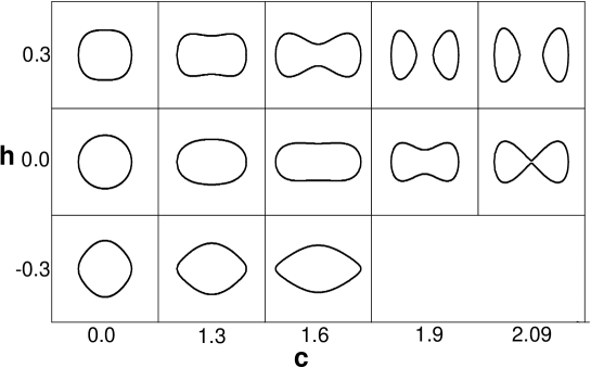
The volume is kept constant in the above parametrization for all variations of the nuclear shape. The total length of the longer axis of the density distribution, in units of , simply equals . The parameter describes the variation of the thickness of the neck without changing the length of the nucleus, and is chosen in such a way that the line fits approximately the bottom of the liquid drop valley. Positive values of implies that the neck formation starts for a lower value of as compared to the the case of and hence scission of the nucleus into two fragments also takes place for a lower value of . Inclusion of the neck degree of freedom is thus expected to accelerate the fission process. When , one has a set of oblate , and prolate ellipsoids. When , one obtains a family of symmetric shapes ranging from the spherical shape to two fragment shapes . For , and are connected by the following expression[130],
| (2.5) |
This parametrization describes separated shapes when .
2.3 Langevin equation for fission
The Langevin equation is the equation of motion of a Brownian particle in a viscous medium placed in an external potential field and is essentially given by the Euler-Lagrange equation where a dissipative force and a random force are included in the force balance equation. In the case of nuclear fission, the fission degree of freedom is considered as the Brownian particle while the friction and random forces arise out of the interaction of the fission degrees of freedom with the rest of the nuclear degrees of freedom, as we have discussed in the previous chapter. The two dimensional Langevin equation in coordinates has the following form[101]
| (2.6) |
with summation from 1 to 2 (c & h) over repeated indices; corresponds to and corresponds to . is the free energy of the system and and are the shape-dependent collective inertia and dissipation tensors, respectively. The random force represents the random part of the interaction between the fission degrees of freedom and the intrinsic degrees of freedom (considered as a thermal bath in the present picture) and is given by the following equation [33, 48],
| (2.7) |
The time-correlation property of is given the following relation,
| (2.8) |
where the strength of the random force is assumed to satisfy Einstein relation (fluctuation-dissipation theorem) which reads as follows
| (2.9) |
where is the temperature of the compound nucleus. It is assumed that [33, 48]
| (2.10) |
Comparing the above equations (Eqs. 2.7 to 2.10), it follows that
| (2.11) |
The conservative force is usually specified from an appropriate nuclear model while the friction force is treated as a phenomenological quantity. These different inputs to the Langevin equation as chosen in our dissipative dynamical model will be described in detail in the following sections.
2.3.1 Potential
The potential energy enters into our calculation through its dependence on the deformation coordinates and . It could in principle be obtained from a microscopic mean-field calculation at a finite temperature. This type of Hartee-Fock calculation using a reasonable effective nucleon-nucleon interaction of the Skyrme type or Gogny type at every point in the multidimensional deformation space, demands tremendous computer time even with the most powerful computers and hence performing such a computation for the present purpose is not attempted. To perform the same kind of calculation even on the level of a self consistent semiclassical approximation like the Extended Thomas-Fermi (ETF) method [131] at finite temperature [132], which would describe the average nuclear structure without shell oscillations, would also be far too time consuming with advanced computers. We have therefore used a still simpler semiclassical approach where the deformation dependent potential energy is obtained from the finite range liquid drop model [133] with the parametrization of Myers and Swiatecki [134]. In the rotating liquid drop model[135], the nucleus is assumed to be formed of an incompressible fluid with a constant charge density and a sharp surface, which rotates as a rigid body. There are three important contributions to the deformation-dependent potential energy in the liquid drop model: surface tension energy (arising from saturating short range nuclear forces) which tends to minimize the surface area of the nucleus, repulsive Coulomb energy(arising from mutual repulsion of protons) which tends to distort or disrupt the nucleus, and rotational energy which also favours disruption because large moments of inertia are energetically favoured. The basic assumption in the liquid drop model is that the surface thickness and the range of the force should be much smaller than any geometrical parameter of the configuration under consideration. This assumption breaks down in the highly deformed shapes of a fissioning nucleus with small neck where the neck dimension becomes comparable to small surface thickness. In these cases the finite range of the nuclear force and the diffuse surface lead to reduction in the energy which must be taken into account[136]. The following changes are therefore incorporated in the finite-range liquid drop model relative to the liquid drop model, namely (1) the surface energy of the liquid drop model is replaced by the Yukawa-plus-exponential nuclear energy, which models effects of the finite range of the nuclear force, nuclear saturation, and the finite surface thickness of real nuclei[136]; (2) the Coulomb energy is calculated for a charge distribution with a realistic surface diffuseness[137]; and (3) the rotational moments of inertia are calculated for rigidly rotating nuclei with realistic surface density profiles[137]. The different contributions of the deformation dependent potential energy in the finite range rotating liquid drop model are described briefly as follows.
(i) Yakawa-plus-exponential nuclear energy :
The
surface energy of the liquid drop model suffers from several
deficiencies in attempting to describe real nuclei. The most
important of these is the neglect of proximity effects; that is
there is an unrealistically high surface energy for strongly
deformed shapes and an absence of attraction between separated
nuclei in the liquid-drop model[133]. One important step
for obtaining an improved macroscopic nuclear energy is the
Yukawa-plus-exponential double folding potential[136].
With this technique, using one additional parameter (the range of
the potential) compared to the liquid-drop model, one can describe
suitably heavy-ion scattering potentials, fusion barriers for
light and medium-mass nuclei, the lower fission barriers observed
in nuclei with , and also satisfy the condition for
nuclear saturation[136, 138]. The better reproduction of
the fission barriers with this Yukawa-plus-exponential potential
motivated us to use it in our calculation. The Yukawa-plus
exponential nuclear energy may be written as
| (2.12) |
where , and is the neutron-proton asymmetry. The integrals are over the volume of a sharp surfaced nucleus. The range is the one additional parameter of this modification of the liquid drop model. The value of is determined from average charge radii of nuclei found in electron-scattering experiments, is determined from heavy-ion scattering experiments, while the surface energy and surface asymmetry constants and are determined from fitting the macroscopic fission barriers of nuclei with mass numbers from 109 to 252 at low angular momentum[136, 138]. The values of the constants used here are as follows[133]:
(ii) Coulomb energy :
The sharp surfaced charge distribution of a nucleus is made diffuse by
folding a Yukawa
function with range over a liquid drop distribution, and the
Coulomb energy of the liquid drop model is modified by a
Yukawa-plus-exponential function (almost similar in form as
in the case of surface energy),
proportional to . The range
parameter is chosen to be 0.704 fm. The diffuse surface
correction lowers the Coulomb energy since charge is spread over a
greater effective volume when the surface is made diffuse.
The six dimensional integrals in Coulomb and surface energy are
reduced to three dimensional integrals by Fourier transform
techniques. The axial symmetry of the shape parametrization is
also utilized effectively in simplifying these integrals. The
method used for evaluating the nuclear potential (surface and
Coulomb) is briefly
described in Appendix A.
(iii) Rotational energy :
The rotational energy of a nucleus is given by where is the largest of the
principal-axis rigid body moments of inertia. For a matter
distribution made diffuse by folding a Yukawa function over a
sharp-surfaced one, the rigid body moment of inertia is modified
by the term , where is the range
parameter of the folding function. The same diffuseness parameter
is used for both the charge and the matter distribution and
fm[133].
The fission barriers calculated from this model of potential energy have been found to be within 1 MeV (for the angular momentum values which are sampled in such experiments) of those which optimally reproduce fission and evaporation-residue cross-sections for a variety of nuclei with masses ranging from 150 to above 200[133]. Langevin dynamical calculations of fission fragment mass distribution in fission of excited nuclei is reported in Ref. [139] using two liquid drop models(LDM’s): the LDM with the sharp surface of the nucleus and the finite range LDM and it is seen that the fission fragment mass distributions and their variances calculated with finite-range LDM are in much better agreement with experimental data.
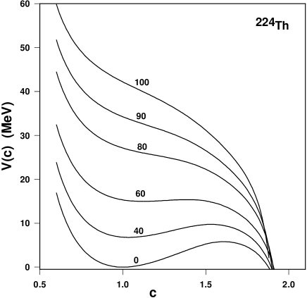
The deformation dependent potential energy which includes contributions from (i) surface energy (ii) Coulomb energy and (iii) rotational energy is plotted as function of the deformation coordinate for different values of angular momentum as marked in Fig. 2.2. It is seen from the figure that the fission barrier decreases with increasing values of angular momentum and gradually vanishes for higher values of . We have not included any shell and pairing effects in our potential. Compound nuclei formed with large angular momentum in heavy-ion collisions of highly excited nuclei ( MeV) will generally also have high internal excitation energy. For sufficiently high internal energies, shell and pairing effects are very small and therefore can be neglected for all practical purposes. The de-excitation of a compound nucleus by particle and gamma emission may however lead to a daughter nucleus with a lower excitation energy where the quantum effects like pairing correlations and shell effects start becoming important. But at such low excitation energies, fission cross section is also very low and also the neutron emission threshold is not reached. The nucleus predominantly cools by photon emission in this energy regime. Since we will mainly be concerned with prescission neutron multiplicity and fission probability, neglecting shell effects in the fission dynamics calculation is expected not to introduce any serious error in our calculation.
2.3.2 Level density parameter
The level density parameter is an important input for our calculations. Fröbrich et al. made an extensive study of different parameterizations available for this crucial quantity and finally considered the form given by Ignatyuk et al. to be the most appropriate for the fission process. We shall use the following level density parameter due to Ignatyuk et al. [140] which incorporates the nuclear shell structure at low excitation energy and goes smoothly to the liquid drop behavior at high excitation energy. In Ignatyuk’s approach the level density parameter is itself taken as a smooth function of mass but with an energy dependent factor which introduces the shell structure explicitly:
| (2.13) |
with
where is the liquid drop level density parameter, determines the rate at which the shell effects disappear at high excitations, and is the shell correction given by the difference between the experimental and liquid drop masses, . We shall further use the shape-dependent liquid drop level density parameter as function of elongation coordinate given as [141] (leaving out the curvature corrections),
| (2.14) |
The choice of the values for the parameters , and the dimensionless surface area by Fröbrich et al.[47] was motivated by the fact that when using a stronger deformation dependence of the level density parameter, e.g. that of Ref. [142], it was not possible to find a universal, i.e. for all systems, the same friction parameter . Hence they selected among the different possibilities the weakest coordinate dependence which is consistent with data. Those values correspond to and [140] which we shall use in our work. The parametrization used for is of the following form[143]:
| (2.15) | |||||
where is related to c & h by Eq. 2.1.
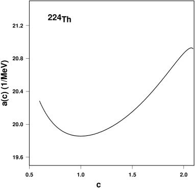
The variation of the level density parameter with the elongation coordinate is shown in Fig. 2.3. The fission rates turn out to be sensitive to the detailed coordinate dependence of the level density parameter. The temperature of the system is also extracted using the level density parameter which in turn dictates the emission of light particles. Thus emission rates therefore also depend on the level density parameter.
In Ref. [144], the level-density parameter and the Helmholtz free energy are calculated using the generalized finite-range liquid drop model(LDM). The finite-range LDM based on the Yukawa-plus-exponential potential was generalized by Krappe[145] to describe the temperature dependence of the nuclear free energy. This dependence is obtained by fitting the results of the temperature-dependent Thomas-Fermi calculation[146] with a finite-range formula. Based on these calculations, the level-density parameter was approximated by a leptodermous-type expression. The coefficients of this expansion are in good agreement with those obtained earlier by Ignatyuk et al.[140]. The results of Langevin dynamical calculations of the mean prescission neutron multiplicity and fission probability are practically the same for the level-density parameter calculated with Ignatyuk’s coefficients as well as the one calculated using the generalized finite-range liquid-drop model[144]. This fact establishes the validity of our dynamical calculations performed with Ignatyuk’s level-density parameter.
2.3.3 Free Energy
The driving potential for a hot thermodynamic system such as the excited nuclei has to be the free energy[24, 143, 147, 148] which can easily be seen from the following arguments. The total energy change is given by where is the work done and is the change in entropy. Using the relation in this formula, one obtains , i.e. the driving force is the negative gradient of the free energy with respect to the fission coordinate at a fixed temperature .
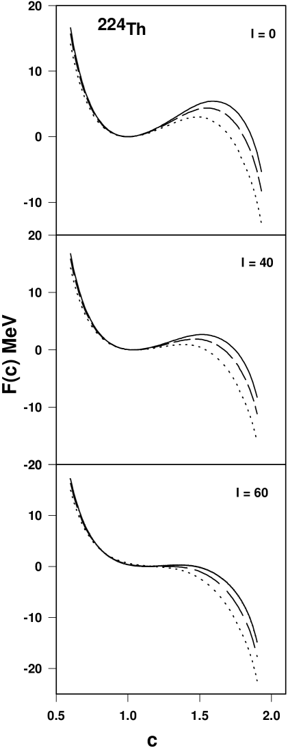
Considering the nucleus as a non interacting Fermi gas, the following expression will be used for free energy (as function of the elongation coordinate ),
| (2.16) |
where is the temperature of the system, is the potential energy and is the coordinate dependent level density parameter. The driving force is thus given by
| (2.17) |
i.e. it consists of the usual conservative force plus a term which comes from the thermodynamical properties of the fissioning nucleus, which enter via the level density parameter , whose deformation dependence is now essential. The properties of the heat bath enter in the description via the temperature , which is calculated from the internal energy and the level density parameter by the Fermi gas relation . Free energy is plotted in Fig. 2.4 for three different temperatures. It is seen from the figure that the fission barrier decreases with increasing temperature for a fixed value of angular momentum . The plot is repeated for three different angular momentum as seen from the figure. It is also seen from comparison of Figs. 2.2 and 2.4 that fission barrier in the free energy profile is lower than that in the potential energy profile and this will have significant impact in the calculation of different observables in fission dynamics of hot nuclei where free energy will be used to generate the driving force.
2.3.4 Inertia
We will make the Werner Wheeler approximation[74, 149] for incompressible irrotational flow to calculate the collective inertia term . We shall follow the work of Davies. et al.[74] for this purpose. The total kinetic energy of the system is given as
| (2.18) |
We specialize here to axially symmetric shapes, for which the velocity is given in cylindrical coordinates by
| (2.19) |
where and are unit vectors in and directions, respectively. The Werner-Wheeler method is equivalent to assuming that is independent of and depends linearly on , i.e., and , where are the generalized velocities and correspond to and in our case. is the value of on the surface of the shape at the position . By virtue of the equation of continuity, the velocity field for an incompressible fluid satisfies and using this relation it can be shown that the expansion coefficients and are related by the equation . The collective kinetic energy of the system depends on the generalized velocities as
| (2.20) |
where denotes the generalized coordinates that specify the shape of a system and corresponds to and in our case. Substituting the expressions for and in Eq. 2.20 and comparing Eq. 2.18 with Eq. 2.20 , we obtain for the elements of the inertia tensor the result
| (2.21) |
where the primes denote differentiation with respect to z. The expansion coefficients are determined from the condition that for an incompressible fluid the total(convective) time derivative of any fluid volume must vanish. The formula for is given by the following expression
| (2.22) |
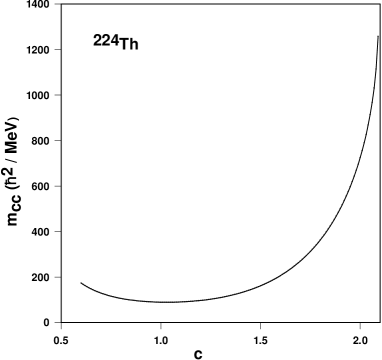
This inertia tensor is then calculated for different values of the collective coordinate and . has three components, namely, , and . Fig. 2.5 shows the variation of the component with elongation . It needs mentioning that our calculations will be essentially in one dimension( coordinate), and hence we will be concerned mainly with the component , the other two being not needed for our purpose. We shall denote by for the sake of simplicity.
2.3.5 Random force R(t)
The instantaneous random force plays a very crucial role in the Langevin description of nuclear fission. Though the initial collective kinetic energy of the fission degrees of freedom may be lower than the fission barrier, as a result of receiving incessant random kicks from the fluctuating force , the fission degrees of freedom can finally pick up enough kinetic energy to overcome the fission barrier. This random force is modelled after that of a typical Brownian motion and is assumed to have a stochastic nature with a Gaussian distribution whose average is zero [33]. It is further assumed that has extremely short correlation time implying that the intrinsic nuclear dynamics is Markovian. Consequently the strength of the random force can be obtained from the fluctuation-dissipation theorem and the properties of can be written as,
| (2.23) |
where is the strength of the dissipation and is the nuclear temperature.
2.4 One-body dissipation
2.4.1 Wall Friction
It is already pointed out in the previous chapter that one-body dissipation is the dominant mode of energy damping in nuclear fission and is considered to be more successful in describing fission dynamics than two-body viscosity [101]. At excitation energies per nucleon much smaller than the Fermi energy domain, the exclusion principle will severely restrict the phase space available for two-body collisions and the one-body mechanism is expected to dominate. Hence we shall use the one-body dissipation for nuclear friction in the Langevin equation. The standard prescription for one-body dissipation is the wall friction which has been introduced in the previous chapter in some detail. However, for realistic applications, it was found [109, 150] that the wall friction overestimates the one body dissipation (as required to fit experimental data for fission of hot nuclei) by an order of magnitude. In order to reproduce simultaneously the measured prescission neutron multiplicities and the variance of the fission fragment mass-energy distribution, the reduction coefficient() of the contribution from a wall formula has to be decreased at least by half of the one-body dissipation strength ( )[151, 152].
In the microscopic derivation of the wall friction it is seen that the energy transferred to particle motion in a dissipative process of very short duration (smaller than the interval between successive collisions between a particle and the wall) is given by the original wall friction. In other words, energy damping is given by wall friction irrespective of the shape of the potential when time available for energy damping is short compared to the time between successive collisions. When the dissipative process lasts longer, a part of the energy transfer could be reversible and the net energy transfer can be shown to depend on the shape of the potential. One of the important assumptions of the wall friction concerns the randomization of the particle motion. It is assumed[73] that successive collisions of a nucleon with the one-body potential give rise to a velocity distribution which is completely random. This is normally satisfied for one body potentials whose shapes are rather irregular. If the particle motion is not fully random, energy transferred to a particle from a time-dependent wall could be partly reversible, resulting in a reduced strength of the wall friction. The classical wall friction was therefore re-examined in order to distinguish between the reversible and irreversible energy transfers. The irreversible energy transfer was identified with the true one body dissipation. The wall friction was modified to describe the irreversible energy transfer and the modified wall friction would be applicable to systems in which particle motion is not fully randomized. Studies of the nature of dynamical systems [153] demonstrated that even simple systems possess a rich phase space structure and classical dynamics can be idealized for the two extreme cases of either fully regular(integrable) or fully chaotic(nonintegrable) motions. Most of the systems of practical interest fall in between the above limiting cases and they are ‘mixed’ systems which display both regular and chaotic(irregular) features. Arvieu et al. [154] pointed out the importance of topology of phase space to characterize the motion of a particle moving in a deformed potential. Blocki et al. [111] showed a strong correlation between chaos in classical phase space and efficiency of energy transfer from collective to intrinsic motion. It was established by their calculations that for slow dissipative processes, wall friction is valid when the intrinsic dynamics is fully chaotic. The wall friction was therefore modified to make it applicable to mixed systems i.e., when mixing in phase space is partial. Following the above line of argument, we shall describe a specific model, namely the Chaos Weighted Wall Friction, in the following sub-section.
2.4.2 Chaos Weighted Wall Friction
Pal Mukhopadhyay[123] introduced a measure of chaos into the classical linear response theory for one body dissipation, developed earlier by Koonin and Randrup [122] and a scaled version of the wall friction, namely the “chaos weighted wall friction” was thus obtained. We shall present a brief account of this model of one-body friction here.
Following the work of Koonin and Randrup, a classical system of independent particles placed in a container with time-dependent walls is considered which is described by Hamiltonian and respectively. Under the linear response approximations which require the validity of a perturbative treatment and the assumption that the relaxation time of intrinsic motion is short in comparison with the time scale for collective motion(adiabatic approximation), the rate of energy dissipation from the collective motion of the wall can be expressed as
| (2.24) |
This equation corresponds to a physical picture in which a particle originating from a point in phase space contributes a dissipation rate equal to the product of the initial impulse received and the sum of all impulses received subsequently along its entire (unperturbed) trajectory . In the above expression is the single particle phase space distribution function governed by the unperturbed Hamiltonian and the factor ensures that for a Fermi-Dirac distribution only particles near the Fermi surface contribute. It was observed that relaxation of the adiabatic approximation to realistic collective speeds reduces the damping by . Therefore the above equation shall give the leading contribution to one-body damping even when the collective and intrinsic time scales become comparable. Considering a leptodermous system in which the nuclear potential is uniform throughout the volume but rises steeply at the surface, the above time integral can be written as a sum of the impulses received by a particle during its successive encounters with the nuclear surface along its unperturbed trajectory. Separating the contribution of the first impulse given to a particle near its point of origin at (local part) from those arising out of the successive reflections from other regions of the nuclear surface (nonlocal part) Koonin and Randrup[122] obtained the energy damping rate as
| (2.25) |
The nonlocal term is determined by the correlation in the velocity field sampled at successive reflection points of a particle trajectory in the unperturbed system. This correlation, in turn, depends on the nature of the velocity field at the cavity surface as well as on the nature of the particle trajectory. It was found that the local and the nonlocal parts completely cancel each other in an integrable system in which particle trajectories are fully regular. This essentially reflects a regular distribution of the velocity fields which results in a strong correlation when sampled at reflection points along a regular trajectory. It is argued that energy transfer to the particle motion described by the regular part of the classical phase space is reversible i.e., energy gained by a particle from the wall is eventually fed back to the wall when particle motion is regular. An integrable system is thus completely non dissipative in this picture and wall friction tends to the limit of zero energy loss. Noninteracting particles in a spherical cavity constitute an example of an integrable system in which particle trajectories are fully regular.
In the case of a non integrable system, on the other hand, where particle dynamics is fully chaotic, the velocity fields sampled by such trajectories are expected to be highly uncorrelated leading to a vanishing nonlocal dissipation. This in turn corresponds to a completely irreversible energy transfer arising from the local term alone and energy dissipation in an irregular system can thus be shown to reduce to the wall friction. Particle trajectories in cavities with octupole and higher multipole deformations follows the full wall friction limit which confirms that the energy damping for irregular systems is entirely determined by the local term. Considering classical particles in vibrating cavities of various shapes, it was demonstrated in[111, 112] that while the energy transfer is much smaller than the wall friction limit in a cavity undergoing quadropule vibration, it reaches the wall friction limit for higher multipole vibrations. Similar conclusions were also reached [104, 114, 115, 116] when the particle motion was treated quantum mechanically, though the quantal energy transfers were found to be somewhat suppressed compared to the classical ones. It was also noted that if the interaction time is too short for any possible transfer of particle energy to the wall after the first collision, the net energy transfer rate would be given by the local term, or, equivalently, the wall friction, irrespective of the system being regular or chaotic.
Most of the physical systems of interest however are neither fully integrable(full regularity) nor fully nonintegrable(complete chaos). The dynamics of such systems display both the characteristic features of regularity and chaos in classical phase space. The measure for the degree of chaos or nonintegrability for mixed systems is usually defined as the relative volume of phase space that belongs to chaotic trajectories. A trajectory is said to be regular when originating from a given point on the cavity wall and moving in a given direction, it closes smoothly in phase space. On the other hand, another trajectory leaving the same point but in a different direction could be a chaotic one which does not close in the phase space. It has already been stated that regular trajectories contribute to zero net dissipation while the dissipation due to the chaotic trajectories correspond to the full wall friction. The dissipation rate in mixed systems can therefore be decomposed into following four terms,
| (2.26) |
The first two terms on the right side represent the local and nonlocal contributions to the dissipation due to the trajectories which are regular and they are expected to cancel each other as noted before. The nonlocal term due to the chaotic trajectories also vanish due to the random nature of the surface velocity components at successive reflecting points as mentioned previously. Therefore we are left with the local term due to the chaotic trajectories and the net dissipation rate amounts to . This term represents the contribution of the chaotic trajectories alone and can be written as
| (2.27) |
where is the fraction of the chaotic trajectories and ( is the normal component of the surface velocity at the surface element ) represents the full strength of the wall dissipation where all trajectories (regular + chaotic) are considered. The details of the derivation can be found in Ref. [123].
The wall friction is thus modified by a factor (chaoticity) which gives the average fraction of trajectories which are chaotic when sampling is done uniformly over the surface. In other words, the chaoticity is used to express the degree of irregularity in the dynamics of the system. This modified or scaled version of the wall friction is known as the ”chaos-weighted wall friction”(CWWF)[123].
The CWWF coefficient will therefore be given as
| (2.28) |
where is the friction coefficient as given
by the original wall friction. This modified version is applicable
for any system lying between a fully regular (, i.e., no
dissipation) and a fully chaotic one (, i.e, original wall
friction). For mixed systems, the dissipation rate depends on the
degree of chaos in single particle motion of the nucleons within
the nuclear volume and it is thus necessary to calculate for
such systems. The chaoticity is a specific property of the
nonintegrability of the nuclear shape. Thus it is required to be
calculated for all possible shapes of the nucleus up to the
scission configuration. In order to calculate the chaoticiy ,
it is required to identify a classical trajectory as a regular or
a chaotic one. For conservative Hamiltonian systems, the methods
which are mostly used to
distinguish between regular and chaotic
trajectories are to investigate
Poincare surfaces of section.
Lyapunov exponents.
In our work we will use the second method to evaluate the chaoticity .
2.4.3 Chaoticity from Lyapunov exponent
One representative feature of a chaotic trajectory is its sensitivity to initial conditions and the consequent exponential divergence of the neighboring trajectories. A typical calculation for chaoticity proceeds as follows. Two chaotic trajectories (systems) having very close initial conditions and governed by the same set of equations of evolution will eventually fall apart very rapidly as the time progresses and will never come back close to each other (except accidently). Here lies the unpredictability of a chaotic system, though governed by deterministic equations and hence the name deterministic chaos in contrast to noise which is statistical in nature. The initial distance (a measure of difference in the initial condition) between two trajectories can diverge or converge as
| (2.29) |
If the value of is zero or negative, the trajectories converge rapidly (integrable system) whereas positive values imply exponential divergence and chaos. For a system with dimensions in phase space there will be such exponents corresponding to each dimension. The coefficient ( to ) is known as the Lyapunov exponent in the limit when time tends to infinity and the initial distance tends to zero. Hence
| (2.30) |
In order to calculate the dissipation according to the chaos weighted wall friction (CWWF), the chaoticity is required for all the deformations through which the nuclear shape evolves with time. The chaoticity for each deformation is obtained by considering particle trajectories in a cavity with the same deformation and distinguishing between the regular and chaotic trajectories. The chaoticity is defined as the average fraction of chaotic trajectories by uniformly sampling the trajectories which originate from the nuclear surface. Hence we calculate it by considering a large number of (typically 1000 or more) trajectories whose starting points on the nuclear surface are chosen at random. The initial coordinates of a classical trajectory starting from the nuclear surface are chosen by sampling a suitably defined set of random numbers such that all initial coordinates follow a uniform distribution over the nuclear surface. The initial direction of the trajectory is also chosen randomly and its Lyapunov exponent is obtained by following the trajectory for a considerable length of time. A particle’s trajectory is specified by giving its initial coordinates and on the nuclear surface and the components , , of its velocity . For a cavity, a trajectory is independent of the magnitude of the velocity, and hence four quantities, namely , and the orientation of (two angles) are sufficient to define the initial conditions of a trajectory. The magnitude of may be used as a convenient unit of velocity. The method[117] of computing the Lyapunov exponent is based on computing numerically the average rate of exponential divergence (or convergence) of two trajectories with nearly identical conditions (differing only by a small value greater than some predetermined noise threshold), in the limit when the difference between the two initial conditions tends to zero and the time over which the averaging is performed tends to infinity. In general some of the exponents may be positive and some negative. If positive exponents are present, the largest of them will eventually dominate the divergence between trajectories and it will control the exponential instability leading to chaos. In the case of regular trajectories the exponent is zero. The procedure consists in evolving numerically two close trajectories originally separated in phase space by , for a given short interval , after which the magnitude of their separation is scaled back to . The procedure is then repeated times. The largest Lyapunov exponent can be found from the limiting procedure
| (2.31) |
where is the square of the phase space separation between two trajectories after time . The result turns out to be essentially independent of the direction in phase space of the original displacement . In our case the length of the time interval was chosen to be ( being the radius of the spherical system), i.e., =0.5, when time is measured in units of . Each trajectory is identified either as a regular or as a chaotic one by considering the magnitude of its Lyapunov exponent and the nature of its variation with time. Operationally, a trajectory is deemed chaotic if for ,(), saturates to finite values and the value is greater than . The length of duration is found to be sufficient for this decision since for intervals longer than this time, Lyapunov exponent is found to be tending rapidly to zero for regular trajectories. For other trajectories recognized as chaotic, it stays at much higher and more or less steady value. With this method, a large number of trajectories(Lyapunov exponent calculated for each trajectory by following it for the time ) is sampled for each shape of the cavity. Thus after marking and counting the chaotic trajectories (those trajectories for which ) out of the total number of trajectories sampled, the measure of chaoticity for the deformation determined by the ratio of chaotic trajectories to the total number (say N) of sampled trajectories is given by
| (2.32) |
The value of changes from 0 to 1, as the nucleus evolves from a spherical shape to a highly deformed one.
The chaos parameter defined so far is a classically defined quantity which is calculated by sampling trajectories in the classical phase space. For the corresponding quantum system, the chaos parameter is obtained from a measure of the fluctuations of the single particle energy spectrum. For mixed systems, it has been argued that [155] that in the semiclassical limit a spectrum should consist of regular and irregular parts that are associated with the classical regular and irregular regions of phase space.
Using the values of chaoticity calculated as above, the CWWF friction was subsequently found [156, 157] to describe satisfactorily the collective energy damping of cavities containing classical particles and undergoing time dependent shape evolutions. Thus suppression of the strength of the wall friction achieved in the CWWF suggests that lack of full randomization(lack of chaos) in single particle motion can provide an explanation for reduction in strength of friction for compact nuclear shapes as required in the phenomenological friction of Ref. [85]. This motivated us to use the CWWF for nuclear dissipation in fission dynamics which is the main aim of the present thesis. In the present work, the chaoticity is calculated over a range of shapes from oblate to the scission configuration (at c=2.09 where neck radius becomes zero) at small steps of c, the elongation coordinate. Fig. 2.6 shows the calculated values of the chaoticity which will be subsequently used to obtain the chaos-weighted wall friction. Variation of chaoticity with elongation coordinate is plotted, while the coordinate corresponding to the neck degree of freedom is chosen to be zero (). Very small values of chaoticity for near-spherical shapes() implies a strong suppression of the original wall friction for compact shapes of the compound nucleus. Chaoticity, however increases as the shape becomes more oblate or changes towards the scission configuration.
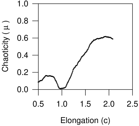
2.4.4 Window Friction and Center of mass correction to Wall Friction
The wall friction assumes isotropic velocity distribution of particles with respect to average drift velocity of the nucleus. In the final stages of fission, the formation of a neck restricts the free passage of particles from one half of the system to the other and the effect of this restriction is that particles bombarding surface elements of each part of the system come mostly from that part and the system is characterized by a leftward as well as a rightward drift. The relevant value of , the normal component of wall velocity with respect to the drift velocity, for the left part of the system is no longer the normal surface velocity with respect to bulk of the whole gas (which is at rest) but the velocity with respect to the leftward moving part. This enforces a correction in the normal velocity of the wall called the center-of-mass motion correction and the normal velocity of the surface element w.r.t particles about to strike it will be (), where is the relative velocity of the part under consideration with respect to the center-of-mass of the nucleus which is at rest[106].
The window friction is expected to be effective after a neck is formed in the nuclear system [106]. When the two halves are in relative motion due to leftward and rightward drifts, any particle passing through the window will damp the motion because of the momentum transferred between the systems. The dissipation rate due to window formation is given by the following expression[73]
| (2.33) |
where and are the components of along and at right angles to the normal through the window and is the area of the window. The radius of the neck connecting the two future fragments should be sufficiently narrow in order to enable a particle that has crossed the window from one side to the other to remain within the other fragment for a sufficiently long time. This is necessary to allow the particle to undergo a sufficient number of collisions within the other side and make the energy transfer irreversible. The window friction should be very nominal when neck formation just begins. Its strength should increase as the neck becomes narrower, reaching its classical value when the neck radius becomes much smaller than the typical radii of the fragments. Very little is known regarding the detailed nature of such a transition, i.e., at which point to switch on the window friction. In our calculation, a transition point is defined in the elongation coordinate beyond which window friction will be switched on. The assumption is that the compound nucleus evolves into a binary system beyond and accordingly correction terms for the motions of the centers of mass of the two halves will be added to wall friction and the window friction will be switched on as well for . It is noted that while the window friction makes a positive contribution to the wall friction for , the center of mass motion correction reduces the friction. These two contributions thus cancel each other to a certain extent and hence, the resulting wall-and-window friction is not very sensitive to the choice of the transition point. This point is explored by the following calculation. The transition point can lie anywhere between (where neck formation just begins) and (scission point). Calculations for fission probability and prescission neutron multiplicity were performed with different values for beyond 1.5, the calculated values were in agreement within . Therefore, the values of is not very critical for our purpose. A value for is chosen at the point when neck radius is half the radius of either of the would be fragments. The value of is thus halfway between its lower and the upper limit in terms of the neck radius.
2.4.5 Friction coefficient
We shall use the following expressions for the wall-and-window friction coefficients in one dimension ()[158],
| (2.34) |
where
| (2.35) |
and
| (2.36) |
where
| (2.37) | |||||
and
| (2.38) |
In the above equations, is given by Eq. [2b], is the mass density of the nucleus, is the average nucleon speed inside the nucleus. at zero temperature is defined as
| (2.39) |
with the Fermi momentum and is
the nuclear matter density.
, are the positions of the
centers of mass of the two parts of the fissioning system relative
to the center of mass of the whole system. and
are the two extreme ends of the nuclear shape along the axis
and is the position of the neck plane that divides the
nucleus into two parts. In the window friction coefficient,
is the distance between centers of mass of
future fragments and is the area of the window
between the two parts of the system.
The wall friction coefficients given by (Eqs. 2.35 and 2.37) are obtained [73] under the assumption of a fully chaotic nucleon motion within the nuclear volume. However, a fully chaotic motion is achieved only when the nuclear shape is extremely irregular whereas the nucleon motion is partly chaotic in varying degrees for typical nuclear shapes through which a nucleus evolves when it undergoes fission. We have already argued in the preceding section that for such cases, the chaos weighted wall friction () should be employed instead of the original wall friction. Accordingly, we shall replace Eqs. 2.35 and 2.37 by their chaos weighted versions and the chaos-weighted wall-and-window friction (denoted henceforth by ) is subsequently obtained as
| (2.40) |
and
| (2.41) |
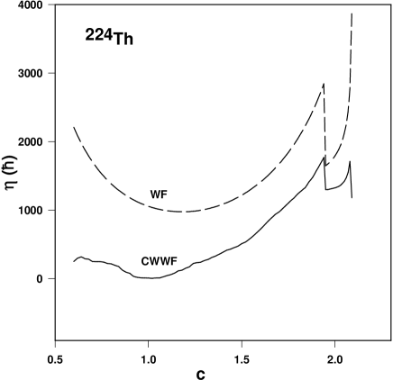
Fig. 2.7 depicts the variation of the friction coefficient with elongation for both CWWF and WF.
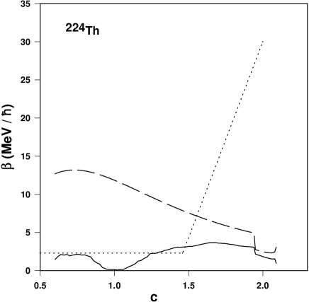
Defining a quantity ( corresponds to the inertia component ) as the reduced friction coefficient, its dependence on the elongation coordinate is shown in Fig. 2.8 for both the WF and CWWF for the 224Th nucleus. A strong suppression of the original wall friction for compact shapes of the nucleus can be immediately noticed in the CWWF. This implies that the friction is very small for near spherical shapes (), the physical picture behind which is as follows. A particle moving in a spherical mean field represents a typical integrable system and its dynamics is completely regular. When the boundary of the mean field is set into motion (as in fission), the energy gained by the particle at one instant as a result of a collision with the moving boundary is eventually fed back to the boundary motion in the course of later collisions. An integrable system thus becomes completely nondissipative in this picture resulting in a vanishing friction coefficient. This aspect has been investigated extensively on earlier occasions [122, 123] and has been found to be valid for any generic integrable system. The reduction in the strength of the wall friction is shown in Fig. 2.8 along with the phenomenological reduced friction obtained in Ref. [150] to fit experimental data. The reduction in the strength of the phenomenological friction is found to be very similar to that obtained from chaos considerations. Though the CWWF agrees qualitatively with the phenomenological friction for , it is beyond its scope to explain the steep increase of phenomenological friction for . We shall discuss this point further while presenting the results in chapter 4.
The strong shape-dependence of the CWWF can have some interesting consequences. In a dynamical description of fission, a compound nucleus spends most of its time in undergoing shape oscillations in the vicinity of its ground state shape before it eventually crosses the saddle and proceeds towards the scission point. Since the spin of a compound nucleus formed at a small excitation (small temperature) is also small, its ground state shape is nearly spherical and in this region the CWWF is also small. Conversely, higher spin values are mostly populated in a highly excited compound nucleus (high temperature) making its ground state shape highly deformed and thus it experiences a stronger CWWF. Therefore, if one uses a shape-independent friction in a dynamical model of fission, its strength has to increase with increasing temperature in order to give an equivalent description to that provided by the temperature-independent but shape-dependent CWWF. In fact, it was observed in Ref. [159] that a shape-dependent friction fits the experimental data equally well to that achieved by a strong temperature-dependent friction. Since there is a physical justification for shape-dependence in nuclear friction from chaos considerations, it is quite likely that the above strong temperature-dependence, at least a substantial part of it, is of dynamical origin as explained in the above and thus is an artifact arising out of using a shape-independent friction.
It must be pointed out, however, that one would expect a temperature-dependence of nuclear friction from general considerations such as larger phase space becoming accessible for particle-hole excitations at higher temperatures. In a microscopic model of nuclear friction using nuclear response function, Hofmann et al. [100] have obtained a nuclear friction which depends upon temperature as (leading term). This may be compared with the empirical temperature-dependent term of which was found in Ref. [159]. It therefore appears that only a small fraction of the empirical temperature-dependence can be accounted for by the inherent temperature-dependence of nuclear friction while the rest of it has a dynamical origin as we have discussed in the above. In fact it shown in Ref. [160] that in hot rotating where saddle to scission emission dominates the prescission particle and -ray spectra, the extracted nuclear dissipation coefficient is found to be independent of temperature and large dissipation during the saddle to scission path provides good fit to the -ray spectra. Similar conclusion is reached in Ref. [161] for where the friction parameter is found to be smaller inside the saddle and increases sharply outside the saddle in order to match experimental data. In the present work, we shall not consider any empirical temperature-dependence of the CWWF or WF in order to study solely the effects of shape-dependence. In what follows, we shall use both the WF and CWWF in a dynamical model of fission and shall investigate the effect of the reduction in the CWWF strength on prescission neutron multiplicity, fission probability as well as evaporation residue cross section.
Chapter 3 Fission widths of hot nuclei using Langevin dynamics
In this chapter, a detailed systematic study of the fission rates is made using both chaos-weighted wall friction(CWWF) and wall friction(WF) in the Langevin equation for different spins and temperatures of the compound nucleus. Similar studies of fission rates using different versions of friction is not found in the literature except for the work of Abe et al. [48, 162] where time dependent fission rates were calculated using both the two-body viscosity and the wall friction in the Langevin equation. The aim of the present study is two fold. First, the effect of introducing the chaos factor in nuclear friction parameter on fission rates will be examined at different excitation energies and spins of the compound nucleus. The effect of the choice of different scission criteria on fission rates will also be investigated. The second one concerns a parametric representation of the numerically obtained fission width, the need for which arises as follows. Fission width is an essential input along with particle and widths for a statistical theory in the stationary branch of compound nucleus decay. Kramers [8] obtained an analytical expression for the stationary fission width assuming a large separation between the saddle and scission points and a constant friction. Gontchar et al. [143, 150] later derived a more general expression taking the scission point explicitly into account but still assuming a constant shape independent friction coefficient. The CWWF however is not constant and is strongly shape dependent and hence the corresponding stationary fission width cannot be analytically obtained. Thus it becomes necessary to find a suitable parametrization of the numerically obtained stationary fission widths using CWWF in order to use them in the statistical regime of the compound nucleus decay. In the next section, the procedure for calculating the fission rates by numerically solving the Langevin equation is given. The results of our calculation will be presented in section 3.2 while a summary of the chapter will be given in the last section.
3.1 Solving the Langevin equation to calculate fission rate
3.1.1 Inputs to the equation
We have discussed in details the Langevin equation along with the various inputs of our model in the last chapter. The same definitions and notations will be followed henceforth. The shape parameters as suggested by Brack et al. [129] will be taken as the collective coordinates for the fission degree of freedom. We shall further assume in the present work that fission would proceed along the valley of the potential landscape in coordinates though we shall consider the Langevin equation in elongation coordinate alone in order to simplify the computation. Consequently, the one-dimensional potential in the Langevin equation will be defined as at valley. The potential is calculated over a grid of values and the valley of the minimum potential is located. The potential values along this valley are used in solving the Langevin equation. Other quantities such as inertia and friction will also be similarly defined. We shall, therefore, proceed by considering and its conjugate momentum as the dynamical variables for fission for our present study and the coupled Langevin equations in one dimension will be given as
| (3.1) |
The different inputs to the Langevin dynamics, namely the shape dependent collective inertia , the friction coefficient , the free energy of the system , and the random force are described in detail in the previous chapter. The usual wall friction (WF) as well as its modified version CWWF will both be used for the friction coefficient in order to study the effect of introducing the chaos-factor in CWWF. The random force is given by , where the diffusion coefficient is related to the friction coefficient through the Einstein relation . In this framework the temperature is simply a measure of the non-collective part of the nuclear excitation energy and related to the later by the usual Fermi gas relation , where is the level density parameter of the considered nucleus at a nuclear deformation characterized by . The excitation energy itself is determined by the conservation of the total energy as will be discussed afterwards.
3.1.2 Method of solving the equation
The Langevin equation [163] has been applied to many fields of physics. It was solved on several occasions for parabolic potential wells [164, 165]. Recently there has been a publication[166] which showed a general analytical scheme to solve multi-dimensional Langevin equations near a saddle point. Since analytical solutions of the Langevin equation can be derived for quadratic potentials only, it is mostly handled by numerical simulations. The “direct simulation” method is the most commonly used method for solving the Langevin equation. In this method, once the stochastic equation of motion is formulated, it is straightforward to numerically simulate the process in question, using a random number generator to supply the noise. By repeating the simulation with different sequences of random numbers, one obtains independent realizations of the process in question, reflecting the statistical distribution of events. This method however becomes impractical when studying rare outcomes. For instance, while computing the cross-section for the fusion of two heavy nuclei, where the vast majority of realizations will end with the nuclei flying apart, the number of simulations required to obtain even a handful of fusion events may well be prohibitively large. Recently a method based on the idea of importance sampling[167] has been developed for computing the probabilities of rare events for processes described by Langevin equations. However, for our purpose of studying fission dynamics by the Langevin equation, the direct simulation method to solve the equation is quite applicable since fission probabilities of hot nuclei are not too small. We shall follow [33] for the purpose.
The Langevin equation is a stochastic differential equation, which has a rapidly changing force in addition to the ordinary one. The random force has no well-defined derivatives with respect to time and hence the usual methods of solving differential equations such as Runge-Kutta algorithm cannot be utilized for solving the Langevin equation. Therefore it has to be integrated by direct methods. To integrate by the iteration method the Langevin equation is rewritten as follows:
| (3.2) |
where
| (3.3) |
Integrating Eq. (3.2) from to , we have
| (3.4) | |||||
By repeating the same procedure times starting at , we can obtain and at time . At each step, we need , which is a sum of Gaussian random numbers, and thereby is itself a Gaussian random number. Its average and variance can be calculated with the statistical properties of and they are as follows.
| (3.5) |
Thus we can describe by a new Gaussian random number , i.e.
| (3.6) |
where has the following properties (average and variance),
| (3.7) |
The method for generation of random numbers following a particular type of probability distribution is described in Appendix B. The same method is followed here as well as in all other cases where Monte-Carlo simulation is used in the present thesis. Eq. (3.4) is the first order approximation in . In a case such as fission one has to describe the system over a rather long period, which means one has to repeat the small steps many times. The time step is restricted by the friction strength as well as the force or the derivative of the potential. A very small time step of for numerical integration is used in the present work. The numerical stability of the results is checked by repeating a few calculations with still smaller time steps. The solution of Langevin equation of a free Brownian particle obtained by this method and its comparison with the analytical solution is presented in Appendix C. The close agreement of the numerical and the analytical solution confirms validity of the algorithm used in solving the Langevin equation. The units and dimensions used for different dynamical variables in the Langevin equation are described in details in Appendix D.
3.1.3 Initial conditions and scission criteria
Initial conditions
The initial
distribution of the coordinates and momenta are assumed to be
close to equilibrium and hence the initial values of are
chosen from sampling random numbers following the
Maxwell-Boltzmann distribution. Starting with a given total
excitation energy () and angular momentum () of the
compound nucleus, the energy conservation in the following form,
| (3.8) |
gives
the intrinsic excitation energy and the corresponding nuclear
temperature
at each step of the fission
process(each integration step).
The centrifugal potential is included in in the above equation.
Once the initial conditions are fixed one can integrate the
system of equations of motion, i.e. Eq. (3.1) using their
finite difference version i.e., Eq. (3.4). At each time step
one draws a random number from a gaussian
distribution which defines the fluctuating force and thus
generates a trajectory in the variable .
Scission criteria
“Scission” implies a transition from a continuous nuclear
configuration (that becomes unstable for a number of reasons)
to a configuration in which the nuclear system consists of
separated shapes.
The scission configuration is determined by the intersection
points of the stochastic Langevin trajectories of the fissioning
system, with the scission surface in the coordinate subspace.
For an arbitrary dimensional model the crucial problem is how
to define the scission surface. In fact, at the present time
there is no unambiguous criterion of the scission condition.
The condition of zero neck radius can be considered as one (the
simplest) of the scission conditions. However, this definition is
unsatisfactory because
the description of nucleus
based on liquid-drop model looses significance when the neck
radius becomes comparable with the distance between nucleons.
Hence, it is often supposed [129, 168, 169] that the
scission occurs at a critical deformation with a relatively thick
neck. Physical arguments lead to determine the scission surface as
the locus of points at which the following equation is satisfied:
| (3.9) |
This means that stability against variations in the neck
thickness is lost. Such a criterion of scission can be called the
criteria of instability of the nucleus with respect to variations
in the thickness of its neck [43, 129, 170, 171].
It should be noted that this scission condition corresponds to the
shapes of the fissioning nucleus with a finite neck radius, with
on the average [129, 168, 172], where is the
radius of the spherical compound nucleus and is given by
, A being the mass number of the fissioning nucleus.
Another acceptable and physically sensible criterion is based on
the equality of the Coulomb repulsion and the nuclear attraction
forces between future fragments. It was shown in [75]
that this scission condition leads to scission configurations for
the actinide nuclei with approximately the same neck radius
equaling . In Ref. [173], a probabilistic
criterion is proposed for the scission of a fissile nucleus, where
the probability is estimated by considering scission as a
fluctuation. The effect of the probabilistic criterion of
nuclear-scission on fission-process observables, such as the
moments of the mass-energy distribution of fission fragments and
prescission neutron multiplicity is demonstrated and it is shown
that the Strutinsky criterion[168], according to which
nuclear scission occurs at a finite neck radius of , is a
good approximation to the probabilistic scission criterion in
Langevin dynamical calculations employing reduced wall friction,
with the reduction factor being less than .
These arguments
led us to choose the scission criterion for our work as those
configurations of the fissioning nucleus where the nuclear shapes
have finite neck radius of . However, it is worthwhile to
notice that results of fission dynamics of hot nuclei obtained
with this scission criterion and those with the criterion of zero
neck radius do not vary much.
3.1.4 Fission Rate
A Langevin trajectory will be considered as undergone fission if it reaches the scission point (corresponding to the scission criteria defined above) in course of its time evolution. The calculations are repeated for a large number (typically 100,000 or more) of trajectories and the number of fission events are recorded as a function of time. At each iteration step, we calculate the probability of the system remaining as compound nucleus, , i.e, number of samples with divided by the total number of samples, and then calculate the fission rate as follows,
| (3.10) |
As the rate calculated at each time step is still fluctuating, a time averaging is made over time as
| (3.11) |
The fission width is given by .
The procedure described in this section to compute the fission rate is implemented in a computer code called FISSWDTH developed by us and is used for the numerical calculation presented in the next section. A brief description of FISSWDTH is given in Appendix F.
3.2 Results
A typical Langevin trajectory of nucleus which has reached the scission point and has ended up as a fission event is shown in Fig. 3.1 (upper panel). Another trajectory, the kind of which is less frequent, is shown in the lower panel of the same figure. The Langevin trajectory in this case crosses the saddle point and after spending some time beyond the saddle point drifts back into the potential pocket again. Such trajectories may or may not finally reach the scission point within the observation time and corresponds to a to-and-fro motion across the saddle and essentially portrays the stochastic nature of the dynamics. This point is further illustrated in Fig. 3.2 where time development of the fission rates are plotted.
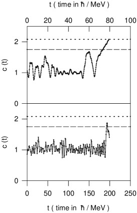
Two different criteria are used to define a fission event here. The filled circles correspond to fission events defined as those trajectories reaching the scission point whereas the open circles correspond to those crossing the saddle point. The fission rate is very small for both the cases at the beginning when the compound nucleus is just formed and the Langevin dynamics has just been turned on. Subsequently the fission rate grows with time and after a certain equilibration time it reaches a stationary value which corresponds to a steady flow across the barrier. The fission rate defined at the saddle point reaches the stationary value earlier than that defined at the scission point. The time difference between them gives the average time of descent from the saddle to the scission.
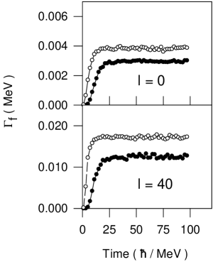
This observation was also made in earlier works [162]. The main purpose of the present discussion is to investigate the role of backstreaming in the fission process. It is observed in Fig. 3.2 that the stationary fission rate at saddle point is higher than that at the scission point. The difference between these two stationary rates can be regarded as due to backstreaming. The backstreaming is thus small compared to the steady outward flow though it is not negligible. This also shows that crossing the saddle point is not an adequate criteria for fission in stochastic calculations and can lead to an overestimation of the fission rate.
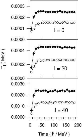
The fission rates calculated with chaos weighted wall-and- window friction is next compared with those obtained with wall-and-window friction. The calculations were performed for a wide range of spin and temperature of the compound nucleus. Fig. 3.3 shows the fission widths at three spins of the compound nucleus . The effect of suppression in the chaos weighted wall friction shows up as an enhancement by about a factor of 2 of the stationary fission rates. Similar enhancement of the stationary fission rate calculated with chaos weighted wall-and-window friction in comparison with that obtained with wall-and-window friction are also observed for a wide range of compound nuclear spin and temperature. The enhancement factor (of about 2) remains almost the same when different choices of are used in the window friction.
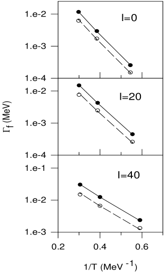
We next systematically extracted the stationary fission widths at different temperatures for a given spin of the compound nucleus. This was done by taking the average of the fission rates in the plateau region. These fission rates are essentially the Kramers’ limit of the Langevin equation under consideration and we expect the stationary fission widths to depend upon the temperature as for a given spin () of the compound nucleus where is the height of the fission barrier in the free energy profile and is a parameter. Such a dependence of stationary fission widths on temperature was indeed found and is shown in Fig. 3.4. The parameter can now be extracted by fitting the calculated fission widths with the above expression.
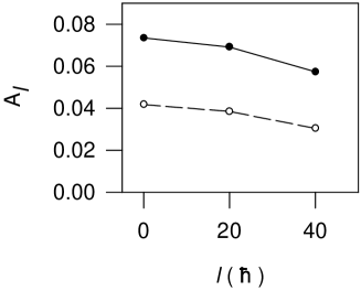
Subsequently we looked into the dependence of the parameter on , a few typical plots of which are shown in Fig. 3.5. The variation of with the spin is plotted both for chaos-weighted wall friction (solid circles) and wall friction(open circles). The nature of variation is similar for both types of friction, while the magnitudes differ almost by a factor of 2 which is expected from the enhancement observed in the stationary fission rates with CWWF (Fig. 3.3). Using these values of , one can now obtain this parameter value for any arbitrary spin by interpolation. Even with a limited number of calculated values, the interpolated values will be quite reliable since depends on rather weakly as can be seen in Fig. 3.5. Consequently it becomes possible to extract the fission width of a compound nucleus of any given temperature and spin from a set of a limited number of calculated widths. This fact will be very useful in statistical model calculations where fission widths are required at numerous values of temperature and spin which are encountered during evolution of a compound nucleus. Therefore in such cases where analytical expressions for fission widths cannot be obtained, the above systematics can generate fission widths from a limited set of calculations.
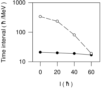
Next we will demonstrate the importance of dynamical models at higher angular momentum. Two time scales are of physical significance in the Langevin description of dynamics of fission. One is the equilibration time , the time required to attain a steady flow across the barrier. The other is the stationary fission life time . Fig. 3.6 shows these time intervals for different values of spin of the compound nucleus . At very small values of spin, the fission life time is many times longer than the equilibration time and one can neglect the equilibration time. This means that a statistical theory for compound nuclear decay is applicable in such cases. On the other hand, and become comparable at higher values of the compound nuclear spin and this corresponds to a dynamics dominated decay of the compound nucleus. Statistical models are not meaningful in these cases and dynamical descriptions such as Langevin equation become essential for fission of a compound nucleus. The results described in this section is reported in Ref. [174].
Before concluding this chapter, we would like to point out that our approximation of restricting the calculation to one-dimension is a reasonable one. This is so because it has been found in earlier works[162] that the fission rate in two-dimensional and one-dimensional cases differ by not more than while the stationary fission rate predicted by CWWF and WF vary by more than . Moreover, we have also checked that the prescission neutron multiplicity and fission probability change by less than when the input fission rates are changed by . Therefore we estimate that the uncertainty associated with our calculation is rather small allowing us to compare our results with experimental data, as we shall do in the next chapter.
3.3 Summary
In the preceding sections, we have presented a systematic study of fission widths using the Langevin equation. Among the various physical inputs required for solving the Langevin equation, we paid particular attention to the dissipative force for which we chose the wall-and-window one-body friction. We used a modified form of wall friction, the chaos weighted wall friction, in our calculation. The chaos weighted wall friction took into account the nonintegrabilty of single particle motion in the nucleus and it resulted in a strong suppression of friction strength for near spherical shapes of the nucleus. The fission widths calculated with chaos weighted wall friction turned out to be about twice the widths calculated with the normal wall friction. The chaos weighted wall friction thus enhances the fission rate substantially compared to that obtained with normal wall friction.
We further made a parametric representation of the calculated fission widths in terms of the temperature and spin of the compound nucleus. It was found that this parameterized form can be well determined from the fission widths calculated over a grid of spin and temperature values of limited size. This fact would make it possible to perform statistical model calculation of the decay of a highly excited compound nucleus where the fission widths are to be determined from a dynamical model such as the Langevin equation. When the friction form factor has a strong shape dependence as in the chaos weighted wall friction, the corresponding fission widths cannot be obtained in an analytic form. In such cases, the frequently required values of the fission width in a statistical model calculation can be made economically accessible through the parameterized representation of the fission width which has to be obtained in a separate calculation similar to the present one. In this calculation of fission rates, we restricted our investigations to the nucleus as a representative example. This nucleus has been experimentally formed at a number of excitation energies [62, 175, 176]. The fission probability and the prescission neutron and multiplicity were measured in these experiments. These quantities can be calculated in a statistical model which requires the fission width as well as the neutron and emission width as inputs to the calculation. In particular, the input fission width plays a critical role in order to reproduce the experimentally determined prescission neutron and multiplicities at high excitation energies(typically a few tens of MeV or higher) in statistical model calculations. While the neutron and widths can be obtained from standard Weisskopf formula [85], a dynamical theory is required to calculate the fission width of the hot compound nucleus. The work reported in this chapter is a step in this direction and the application of these parametrized fission widths (described in this chapter) in dynamical calculations to reproduce experimental data is reported in the next chapter.
Chapter 4 Prescission neutron multiplicity and fission probability from Langevin dynamics of nuclear fission
The Langevin equation has been used extensively in the recent years [48, 85, 152, 177] in order to explain the prescission neutron multiplicity and fission probability of highly excited (typically a few tens of MeV and above) compound nuclei formed in heavy-ion induced fusion reactions. It was shown by Fröbrich and his coworkers[150] that the wall friction cannot reproduce simultaneously experimental data for excitation functions of prescission neutron multiplicity and fission probability. It was found that different values of the reduced friction parameter () ranging from to was required to fit experimental data for different systems(compound nucleus). This is not a satisfactory situation because it is essential that a physically meaningful reduced friction coefficient should be a universal parameter for different systems. This realization led to introduce shape dependence in the friction coefficient and this shape dependent empirical friction parameter of Fröbrich successfully explained experimental data for different systems for prescission neutron multiplicity and fission probability simultaneously [150]. The application of the wall-plus-window dissipation to detailed and systematic analysis of the data from fusion-fission reactions have resulted in deduction of the value of (coefficient which reduces the magnitude of wall friction) for light as well as heavy fissioning systems[179]. The conclusions reached are as follows: (i) = for lighter fissioning systems, (ii) = for the heaviest ones in order to get a good fit of the parameters of the fission fragment mass energy distribution, and (iii) a good quantitative description of the prescission neutron multiplicities and angular anisotropy could be achieved for heavier systems for = . This was an indication that the factor by which the wall friction needs to be reduced might depend on the collective coordinate and excitation energy. Shape dependent nuclear friction coefficient is also extracted in Ref. [160, 161] in order to match giant dipole resonance -ray spectra. It has already been mentioned that an empirical suppression in the wall friction coefficient similar to the one demanded by the experimental data is achieved in the chaos weighted wall friction(CWWF) microscopically, based on physical arguments. In the previous chapter, the fission widths have been calculated using the CWWF in Langevin dynamics and are found to be less by a factor of 2 from those calculated by the standard wall friction. This reduction in fission width is expected to influence the fission probability and prescisssion neutron multiplicity favourably and this encouraged us to do a full dynamical calculation coupled with particle evaporation. The main motivation of the work presented in this chapter is to verify to what extent the chaos-weighted wall friction can account for the experimental prescission neutron multiplicity and fission probability data.
The Langevin equation will be solved by coupling it with neutron and evaporation at each step of its time evolution. Following the work of Fröbrich et al. [178], a combined dynamical and statistical model will be used for our calculation in which a switching over to a statistical model description will be made when the fission process reaches the stationary regime. The prescission neutron multiplicity and fission probability will be obtained by sampling over a large number of Langevin trajectories. We shall perform calculations at a number of excitation energies for each of the compound nuclei 178W, 188Pt,200Pb,213Fr, 224Th, and 251Es. A detailed comparison of the calculated values with the experimental data will be presented. We have mainly considered heavier mass nuclei () since for the lighter mass nuclei, fission width is much less than the corresponding neutron widths and hence the prescission neutron multiplicities in those cases are not sensitive to the choice of nuclear friction. It is for the heavier mass nuclei that the neutron and fission widths become comparable and their competition strongly dictates the final observables.
It is worthwhile here to point out a special feature of the present work. We do not have any adjustable parameter in our entire calculation. All the input parameters except the friction coefficients are fixed by standard nuclear models. The chaos weighted wall friction(CWWF) which is used for the nuclear friction coefficient is obtained following a specific procedure [123] which explicitly considers particle dynamics in phase space in order to calculate the chaoticity factor . There is no free parameter in this calculation of friction. In fact, our main aim in this work is to calculate observable quantities using the theoretically predicted friction and compare them with experimental values in order to draw conclusions regarding the validity of the theoretical model of nuclear friction. As it would turn out, our calculation would not only confirm the theoretical model of CWWF, it would also provide physical justification for the empirical values of friction used in other works [150, 160]. The present work is thus expected to contribute significantly to our understanding of the dissipative mechanism in nuclear fission.
The different steps of the combined dynamical and statistical model calculation will be briefly described in the next section. The calculated prescission neutron multiplicities and fission probabilities will be compared with the experimental values in sec. 4.2. A summary of the results will be presented in the last section.
4.1 Combined dynamical and statistical model
4.1.1 Introduction
After the formation of a fully equilibrated compound system in a heavy-ion fusion reaction, the decay of the compound nucleus can follow two different routes. On the first route the nucleus undergoes fission, i.e, it predominantly separates into two heavy fragments (binary fission) which is called a fusion-fission process. During fission the intermediate system evaporates light particles and -quanta until scission when the neck radius is shrinking to zero. These are called prescission particles. After scission the heavy fragments are still excited and continue to evaporate light particles and -quanta. These are called post scission particles. It is possible to distinguish experimentally between pre- and post-scission particles. Along the second decay route the nucleus does not undergo fission and the excitation of the compound nucleus is removed solely by the evaporation of light particles and -rays. The evaporation of light particles of a particular kind stops when the excitation energy has dropped to a value below the corresponding binding energy. The deexcitation of the system thus ends with the formation of the so-called evaporation residues. For -quanta the emission process lasts until zero excitation energy and the lowest possible spin value are reached. During the formation process of the compound system, some light particles can be emitted, which are of increasing importance with increasing bombarding energy. These particles are called pre-equilibrium particles and since our dynamical model starts from the formation of a equilibrated compound nucleus, we do not take into account these pre-equilibrium particles and hence the experimental data should to be accordingly corrected for these pre-equilibrium emission before any comparison is to be made. Another possibility which may happen is that the intermediate complex formed in the collision is not a fully equilibrated compound system and the process is called fast-fission or quasi-fission process. In our model we always assume that an equilibrated compound system is formed and hence we will not deal with fast fission or quasi-fission processes.
4.1.2 Initial conditions
In our calculation, we first specify the entrance channel through which a compound nucleus is formed. In the reaction process, the compound nucleus can be formed with different values of the angular momentum. For starting a trajectory, an orbital angular momentum value () is sampled from a fusion spin distribution as the proper weight function. This spin distribution is usually calculated with the surface friction model[180]. This calculation also fixes the fusion cross section thus guaranteeing the correct normalization of the fission and the evaporation residue cross sections within the accuracy of the surface friction model. Assuming complete fusion of the target with the projectile, and if both the nuclei are assumed to be spherical, the spin distribution of the compound nucleus calculated with the surface friction model is usually found to follow the following analytical form,
| (4.1) |
where is the wavenumber of the relative motion. This is used as the angular momentum weight function with which the Langevin calculations for fission are started. The situation is more complicated if one or both initial nuclei are deformed. In principle one should then consider all possible relative orientations of the nuclei and follow their relative trajectories from an infinite distance up to fusion. We will avoid such cumbersome calculations and restrict ourselves to the simplified procedure by assuming that both target and projectile are spherical in shape. The parameters and should be obtained by fitting the experimental fusion cross sections. It is however found that these parameters for different systems as calculated by the surface friction model, follow an approximate scaling [85] and hence it is not necessary to perform new surface friction model calculations for the spin distributions of each system. We shall, therefore, use the scaled values of these parameters. The quantity scales as
| (4.2) |
when ; and when , the term in the last brackets is put equal to 2.5. is the center of mass energy while is the Coulomb barrier. For , a simple Coulomb ansatz is used which is given by the following relation,
| (4.3) |
with . The diffuseness is found to scale as
| (4.4) | |||||
The initial spin of the compound nucleus will be obtained by sampling the above spin distribution function.
The Langevin equation and the different inputs for the Langevin dynamics is described in chapter 2. In order to integrate the Langevin equations, we need to fix the initial conditions from which the evolution of the compound system starts. It is also assumed that a fully equilibrated compound nucleus is formed at a certain instant and this point of time is fixed as the origin of our dynamical trajectory calculation. The initial distribution of the coordinates and momenta is assumed to be close to equilibrium and hence their initial values are chosen from sampling random numbers following the Maxwell-Boltzmann distribution. The energy available in the center-of-mass frame can be obtained from the beam energy of the projectile and the target and projectile mass. The excitation energy () of the compound nucleus is obtained from in the following manner.
| (4.5) |
where is the -value of the fusion reaction which forms the compound nucleus(CN), and is the mass defect of the respective nuclei. The target and projectile being in their ground states, shell corrections are to be incorporated to get the proper mass defects[181]. The compound nucleus however is formed in an excited state where shell corrections are expected to disappear and hence not included in the mass defect of the compound nucleus. The mass defect of the hot compound nuclei is taken from Ref. [182]. The total energy conservation of the following form,
| (4.6) |
gives the intrinsic excitation energy and the corresponding nuclear temperature at each time step of integration. The centrifugal potential is included in the potential energy in the above equation.
4.1.3 Particle emission
The process of light particle emission from a compound nucleus is governed by the emission rate at which a particle of type (neutrons, protons and -particles) is emitted at an energy in the range before the compound nucleus eventually undergoes fission. Several theoretical approaches have been proposed in order to describe the emission from a deformed, highly excited and rotating nucleus[42, 177, 183, 184, 185].
According to Weisskopf’s conventional evaporation theory [51], the partial decay width for emission of a light particle of type is given by
| (4.7) |
where is the spin of the emitted particle , is the reduced mass with respect to the residual nucleus. is the intrinsic excitation energy of the parent nucleus, is the binding energy of the emitted particle calculated by the liquid drop model [134], is the energy of the emitted particle and is the change of the rotational energy due to the angular momentum carried away by the rotating particle. The procedure for calculation of the binding energy of the emitted particle is given in Appendix E. The level densities of the compound and residual nuclei are denoted by and and is given by the following formula for the level density of a nucleus[147],
| (4.8) |
where is the moment of inertia and is the angular momentum of the rotating system. The level density parameter for particle emission is taken to be deformation independent and is given by . The inverse cross sections are given by Ref. [53],
| (4.9) | |||||
with
| (4.10) |
where is the mass number of the emitted particle . The Coulomb barrier is zero for neutron whereas for the charged particles the barrier is given by
| (4.11) |
with for and deuteron and 1.15 for proton. For the emission of giant dipole -quanta we take the formula given by Lynn[186]
| (4.12) |
with
| (4.13) |
with , and and are the position and width of the giant dipole resonance. Fig. 4.1 shows the plot of comparison of neutron, gamma and fission widths plotted on a logarithmical scale as function of for three different values of angular momentum . The fission width () shown here is calculated by following the procedure described in chapter 3 using CWWF. The competition between neutron and fission width is the main determining factor in deciding the fate of the compound nucleus. At low angular momentum, fission width is much less than the neutron width but with rise of angular momentum the two widths become comparable.
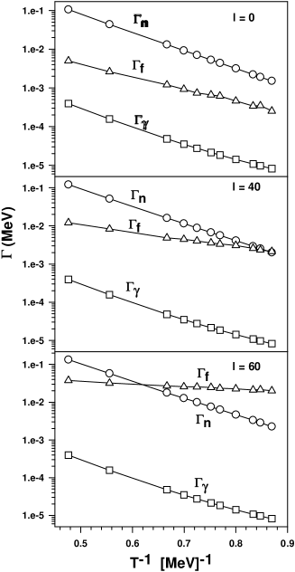
These widths depend upon the temperature, spin and the mass number of the compound nucleus and hence are to be evaluated at each interval of time evolution of the fissioning nucleus.
Once the emission widths are known, it is required to establish the emission algorithm which decides at each time step, along each of the trajectories, whether a particle is being emitted from the compound nucleus. This is done by first calculating the ratio where , and . The probability for emitting any light particle or is given, for a small enough time step , by
| (4.14) |
We shall then choose a random number by sampling from a uniformly distributed set between 0 and 1. If we find , it will be interpreted as emission of either a light particle or a during that interval. If the time step is chosen sufficiently small, the probability of emitting a particle will be small. In this way we guarantee that in each time interval at most one particle is emitted and we avoid to consider the emission of more than one particle in each time interval. In the case that a particle is emitted, the type of the emitted particle is next decided by a Monte Carlo selection with the weights (partial widths). This procedure simulates the law of radioactive decay for the emitted particles. The energy of the emitted particle is then obtained by another Monte Carlo sampling of its energy spectrum by choosing another random number following a probability distribution given by the energy distribution laws in Eqs. 4.7 4.12. The intrinsic excitation energy, mass and spin of the compound nucleus are recalculated after each emission and also the potential energy landscape of the parent nucleus is replaced by that of the daughter nucleus. The spin of the compound nucleus is reduced only in an approximate way by assuming that each neutron, proton or a carries away while the particle carries away of angular momentum. It is assumed that the deformation of the nucleus is not changed due to particle emission. It is evident that each emission of a light particle carries away excitation energy and angular momentum and thereby increases the height of the fission barrier of the residual nucleus which, in turn, renders the fission event less and less probable.
4.1.4 Dynamical model
For each choice of the initial conditions, one generates a separate trajectory which is followed in time dynamically by solving the Langevin equation numerically. The procedure of numerical integration of the Langevin equation which is described in details in the previous chapter is followed here. We will assume in the present work that fission would proceed along the valley of the potential landscape in coordinates, though we shall consider the one dimensional Langevin equation in elongation coordinate alone in order to simplify the computation. This approximation is good enough for the analysis of prescission particle multiplicities and fission probability. The emission of a particle (neutron, proton or ) or a photon and the nature of emission is checked at each time interval. Emitted particles and their energies are registered along a trajectory. Each Langevin trajectory can either lead to fission if it overcomes the fission barrier and reaches the scission point ( is defined in sec. 3.1.3 of the previous chapter) in course of its time evolution. Alternately it will be counted as an evaporation residue event if the intrinsic excitation energy becomes smaller than the fission barrier () and the binding energies of neutron (), proton () and alpha (), i.e., . The calculation proceeds until the compound nucleus undergoes fission or ends up as an evaporation residue. The above scheme can however take an extremely long computer time particularly for those compound nuclei whose fission probability is small. We shall therefore follow a combined dynamical and statistical model, first proposed by Mavlitov et al. [178], in the present calculation. In this model, we shall first follow the time evolution of a compound nucleus according to the Langevin equations as described above for a sufficiently long period denoted by ( is taken as in our model) during which a steady flow across the fission barrier is established. Beyond this period, a statistical model for compound nucleus decay is expected to be a equally valid and more economical in terms of computation. We shall therefore switch over to a statistical model description after the fission process reaches the stationary regime if the compound nucleus does not reach the scission configuration within the time .
4.1.5 Statistical model
When entering the statistical branch we calculate the decay widths for particle emission in the same way as described before. We shall, however, require the fission width along with the particle and widths in the statistical branch of the calculation. This fission width should be the stationary limit of the fission rate as determined by the Langevin equation. Though analytic solutions for fission rates can be obtained in special cases [8, 32, 143] assuming a constant friction, this is not the case with the chaos-weighted wall friction(CWWF) which is not constant and is strongly shape dependent. The fission widths for such shape dependent friction can only be calculated by solving the Langevin equation numerically as described in the previous chapter. Thus it becomes necessary to find a suitable parametric form of the numerically obtained stationary fission widths using the CWWF (and also WF) in order to use them in the statistical branch of our calculation. The details of this procedure is given in chapter 3 and also in Ref. [174], following which we shall calculate all the required fission widths for the present work.
Once the fission widths are known, we use a standard Monte Carlo cascade procedure where the kind of decay at each time step is selected with the weights with () and . This procedure allows for multiple emissions of light particles and higher chance fission. The time step is redefined after each step in the statistical branch as , where . This procedure ensures economy in terms of computation time. The Monte-Carlo procedure chooses the fission route at a certain interval and the trajectory is then counted as a fission event. If the Monte-Carlo procedure does not select the fission channel at a certain interval but selects a particle/ emission, we again recalculate the intrinsic energy and angular momentum, and continue the cascade until the intrinsic energy is min . In this case we count the event as evaporation residue event. The combined dynamical plus statistical calculation is implemented in the fortran code “DYSTNF” (developed as part of the thesis work) which is described in Appendix F. The flow chart of the calculation procedure of this combined dynamical plus statistical model which describes the logical sequence of the actual calculations is described schematically in Appendix G.
4.1.6 Calculation
Following the above procedure, the number of emitted neutrons, protons, alphas and photons is recorded for each fission event. This calculation is repeated for a large number of Langevin trajectories followed by the statistical model and the average number of neutrons emitted in the fission events will give the required prescission neutron multiplicity. The prescission neutron multiplicity is then given by
| (4.15) |
where is the total number of neutrons emitted for those events which have ended in fission and is the total number of fission events. The fission probability will be obtained as the fraction of the trajectories which have undergone fission. The fission cross section is given by the product of fission probability () and the fusion cross section , i.e.,
| (4.16) |
where is the total number of fused trajectories with which we have repeated the whole calculation.
4.2 Results
We have calculated the prescission neutron multiplicity () and the fission probability for a number of compound nuclei formed in heavy-ion induced fusion reactions. We have used both the chaos-weighted wall friction(CWWF) and wall friction(WF) in our calculation. Fig. 4.2 shows the results for prescission neutron multiplicity along with the experimental data. A number of systematic features can be observed from these results. First, the values calculated with the CWWF and WF are very close at smaller excitation energies, though at higher excitation energies, the WF predictions are larger than those obtained with the CWWF. This aspect is present in the decay of all the compound nuclei which we consider here and can be qualitatively understood as follows. The magnitude of the CWWF being smaller than that of the WF, fission rate with the CWWF is higher than that obtained with the WF.

It has been shown in the previous chapter that the stationary fission width with the CWWF is about twice of that with the WF [174]. However at a low excitation energy where a compound nucleus is formed with a low value of spin, the fission barrier is high and fission widths calculated with both CWWF and WF turn out to be many times smaller than the neutron width. This can be seen from Fig. 4.1, where the fission width is calculated using CWWF. The particle multiplicities is decided by the ratio of particle width and the total width . At lower energies, the fission width being much less than the particle width , the particle multiplicity is practically independent of the fission width and hence is insensitive to the particular type (WF or CWWF) of nuclear friction used in calculation of the fission width. The neutrons, therefore, have enough time to be emitted long before a compound nucleus undergoes fission irrespective of its dynamics being controlled by either the CWWF or the WF. This explains the observation of values calculated with CWWF and WF being close at lower excitation energies. Thus the prescission neutron multiplicities are rather insensitive to fission time scales at lower excitation energies. On the other hand, a compound nucleus is formed with a larger spin at higher excitation energies resulting in a reduction of the fission barrier and hence an increase in the fission width. The fission time scales and the neutron lifetimes start becoming comparable at higher excitation energies (refer Fig. 4.1), and the dependence of on fission width becomes sensitive. The fission width calculated with CWWF being about twice than that with WF, time available for evaporation of the neutrons is much less for the former type of friction and hence less neutrons are predicted from calculations with the CWWF than those with the WF. The prescission neutron multiplicity thus becomes capable of discriminating between different models of nuclear friction at higher excitation energies of the compound nucleus.
A similar explanation also holds for the systematic variation of the calculated prescission neutron multiplicities with respect to the mass number of the compound nucleus. We find that the WF prediction for prescission neutrons starts getting distinct from that of the CWWF at smaller values of the excitation energy with increasing mass number of the compound nucleus. Since the fission barrier decreases with the increasing mass of a compound nucleus, the fission time scales and the neutron lifetimes become comparable for heavier compound nuclei at lower excitation energies. This results in a fewer neutrons from calculations with the CWWF than those with the WF as one considers heavier compound nuclei.
A number of interesting points can be noted while comparing the calculated values with the experimental data. For the compound nucleus 178W, the available experimental points [62] are at low excitation energies and therefore, cannot distinguish between the calculated values using the CWWF and WF, which are almost identical. The calculated values slightly overestimate the prescission neutron multiplicity compared to the experimental data. A more extensive set of experimental values for prescission neutron multiplicity are available for the compound nuclei 188Pt, 200Pb, 213Fr and 224Th [62, 187, 188] covering a wider range of excitation energy in which the calculated values with the CWWF and WF differ. Clearly, the CWWF predicted values give excellent agreement with the experimental data for these compound nuclei whereas the WF predictions are considerably higher. However, similar conclusions cannot be drawn for the heavier nucleus 251Es. It appears that the WF predictions are closer to the experimental data [29, 62, 189] whereas the CWWF predictions are somewhat lower. We shall return to this point later for a detailed discussion. For the present, we shall consider the results of fission probability calculations.
The calculated and experimental values of fission probability are shown in Fig. 4.3 for four compound nuclei. While the fission probability for 251Es is almost , for , we shall consider the complimentary cross-section, the evaporation residue cross section separately in the next chapter. Hence they are excluded from the present discussion. The calculated values of fission probability complements the picture of fission dynamics which was obtained while discussing the prescission neutron data. The fission probability is found to be more sensitive to the choice of friction at lower excitation energies than at higher excitations. The CWWF predicted fission probabilities are larger than those from the WF predictions. Moreover, the CWWF predictions are consistently closer to the experimental values of fission probability than those from the WF predictions.

In order to gain further insight into the dynamics of fission, we have also calculated the presaddle and postsaddle (saddle to scission) contributions to the multiplicity of prescission neutrons. Figure 4.4 shows the results obtained with both the CWWF and WF.
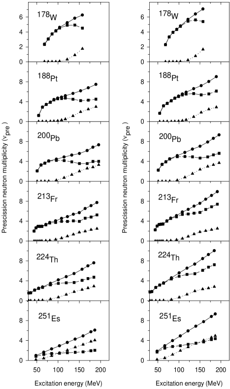
For all the cases, starting from almost zero multiplicity at small excitation energies, the postsaddle contribution increases at higher excitation energies. It is further observed that the postsaddle neutron multiplicities calculated with the CWWF and WF are almost same for all the compound nuclei over the range of excitation energies considered here. This would be due to the fact that the number of postsaddle neutrons depends on the time scale of descent from the saddle to the scission. This, in turn, will depend upon the strength of the friction between the saddle and the scission and we have already seen in Fig. 2.2 that the CWWF and WF are indeed close at large deformations. We shall next compare the presaddle contributions calculated with the CWWF and WF for each of the nuclei under consideration. We immediately notice that the WF predictions are consistently larger than those from the CWWF at higher excitation energies. This gives rise to the enhancement of the WF prediction for total prescission multiplicity compared to that from the CWWF prediction, which we have already noticed in Fig. 4.2 and have discussed earlier. Since the CWWF predicted neutron multiplicities agree with the experimental values for the nuclei 178W, 188Pt, 200Pb, 213Fr, and 224Th, we conclude that the chaos-weighted wall friction provides the right kind of friction to describe the presaddle dynamics of nuclear fission.
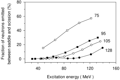
While comparing the relative importance of the presaddle and postsaddle neutrons, we further note that the postsaddle neutrons are more frequently emitted from heavier compound nuclei. For 251Es, most of the prescission neutrons predicted by the CWWF are accounted for by the postsaddle neutrons. The underlying physical picture can be described as follows. When a compound nucleus is formed in a heavy-ion induced fusion reaction, its spin distribution is assumed to be given by Eq. 4.1. If the compound nucleus is formed with a spin at which there is no fission barrier, its transition to the scission point will be essentially considered as postsaddle dynamics. In order to simplify our discussion, let us assume that most of the compound nuclei at a given excitation energy are formed with the spin of Eq. 4.1 and let be the limiting spin value at which the fission barrier vanishes. We can then find a critical excitation energy, , above which becomes greater than and most of the fission dynamics at excitations above this critical value can be considered as comprising of only postsaddle trajectories. In Fig. 4.5, we have plotted the fraction of neutrons emitted in the postsaddle stage as a function of the excitation energy for a number of compound nuclei. The critical excitation energy for each nucleus is also given in this plot. We have used the CWWF predicted neutron multiplicities for this plot where we find that the critical excitation energy decreases with increase in the compound nuclear mass. Thus the dominance of postsaddle neutrons sets in at lower excitation energies for heavier nuclei which, in turn, gives rise to the increase in the fraction of postsaddle neutrons with increasing mass of the compound nucleus.
Though the above discussion clearly establishes the importance of postsaddle neutrons for a very heavy compound nucleus, the number of postsaddle neutrons calculated with the CWWF still falls short of making the total prescission multiplicity equal to the experimental values for 251Es. We consider the apparent better agreement between the WF predicted prescission neutron multiplicity and the experimental data for 251Es as shown in Fig. 4.2 as a mere coincidence and we do not find any physical justification for abandoning the chaos-weighted factor in one-body friction for such heavy nuclei. Instead, we feel that the mechanism of neutron emission in the postsaddle stage requires a closer scrutiny essentially because the nucleus becomes strongly deformed beyond the saddle point. The neutron decay width of such a strongly deformed nucleus could be quite different from that of the equilibrated near-spherical nucleus which we use in our calculation. In particular, the neutron-to-proton ratio is expected to be higher in the neck region than that in the nuclear bulk and this can cause more neutrons to be emitted. Further, dynamical effects such as inclusion of the neck degree of freedom in the Langevin equation can influence the time scale of the postsaddle dynamics and hence the number of emitted neutrons. Such possibilities should be examined in future for a better understanding of the postsaddle dynamics of nuclear fission. The results presented in this section is published in Ref. [158].
4.3 Summary
We have applied a theoretical model of one-body nuclear friction, namely the chaos-weighted wall friction, to a dynamical description of compound nuclear decay where fission is governed by the Langevin equation coupled with the statistical evaporation of light particles and photons. We have used both the normal wall friction and its modified form with the chaos-weighted factor in our calculation in order to find its effect on the fission probabilities and prescission neutron multiplicities for a number of compound nuclei. The strength of the chaos-weighted wall friction(CWWF) being much smaller than that of the wall friction, the fission probabilities calculated with the CWWF are found to be larger than those predicted with the WF. On the other hand, the prescission neutron multiplicities predicted with the CWWF turn out to be smaller than those using the WF. Both the prescission neutron multiplicity and fission probability calculated with the CWWF for the compound nuclei 178W, 188Pt, 200Pb, 213Fr, and 224Th agree much better with the experimental data compared to the predictions of the WF.
We have subsequently investigated the role of presaddle and postsaddle neutrons at different excitation energies for different compound nuclei. It has been shown that the majority of the prescission neutrons are emitted in the postsaddle stage for a very heavy nucleus like 251Es. The CWWF, however, cannot produce enough neutrons to match the experimental prescission multiplicities for such a nucleus. It is, therefore, possible that in the postsaddle region, either the fission dynamics gets considerably slowed down or the neutrons are more easily emitted. These aspects require further studies before we draw conclusions regarding the postsaddle dynamics of nuclear fission.
The presaddle neutrons are however found to account for most of the prescission neutrons for lighter nuclei at lower excitation energies. On the basis of the comparison of the calculated prescission multiplicities with experimental data as given in the preceding section, we can conclude that the chaos-weighted wall friction can adequately describe the fission dynamics in the presaddle region.
Chapter 5 Evaporation residue cross-sections as a probe for nuclear dissipation
Experimental studies of the prescission multiplicities of neutrons [187], rays [89], and charged particles [191] have shown that the fission process is strongly hindered relative to expectations based on the statistical model description of the process, as we have already discussed in the previous chapters. However, it is not possible to infer from these experiments whether the emission of the particles occur mainly before or after the traversal of the saddle point as the system proceeds toward scission. This kind of information could be useful to discriminate between various dissipation models which are strongly dependent on the deformation and shape symmetry of the system. The evaporation probability for hot nuclei formed in heavy-ion fusion reactions can be useful for such purposes which is sensitive only to the dissipation strength inside the fission barrier. As the hot system cools down by the emission of neutrons and charged particles there is a finite chance to undergo fission after each evaporation step. If the fission branch is suppressed due to dissipation there is therefore a enhanced probability for survival which manifests itself as an evaporation residue cross section which is larger than expected from statistical model predictions. It turns out that the evaporation residue(ER) cross-section depends strongly on the strength of the nuclear dissipation whenever it is a very small fraction of the total fusion cross section[192]. The fate of a compound nucleus, i.e., whether it will undergo fission or survive as an evaporation residue is decided mainly within the saddle point. Hence the measurement of evaporation residue formation probability is expected to be a sensitive probe for nuclear friction and may therefore provide the desired separation between presaddle and post-saddle dissipation. It is concluded in Ref. [86] that evaporation residue cross sections give restrictions for possible ( friction parameter) values, and seem to be even more sensitive probes for friction than -rays which is generally considered as a good probe for investigating dynamics in fission.
In a recent work, Diószegi et al. [159] have analyzed the as well as neutron multiplicities and evaporation residue cross-section of 224Th and have concluded that the experimental data can be fitted equally well with either a temperature or a deformation-dependent nuclear dissipation. Interestingly, the deformation-dependence of the above dissipation corresponds to a lower value of the strength of the dissipation inside the saddle and a higher value outside the saddle, similar to the phenomenological dissipation of Ref. [150]. It is worthwhile to note here that our model for nuclear friction i.e., the shape-dependent chaos-weighted wall friction (CWWF) has features similar to the empirical dissipations discussed above. In the present work, we shall employ the CWWF to calculate the evaporation residue excitation function for the 224Th nucleus. Our main motivation here will be to put the CWWF to a further test and verify to what extent it can account for the experimental evaporation residue data which is a very sensitive probe for nuclear dissipation. Calculation will be performed at a number of excitation energies for 224Th formed in the 16O+208Pb system. We have chosen this system essentially because of the availability of experimental data on both evaporation residue and prescission neutron multiplicity covering the same range of excitation energies and the fact that earlier analysis of the evaporation residue excitation function have already indicated the need for a dynamical model for fission of this nucleus [87, 189, 193].
5.1 Calculation
The various inputs required for the model and the different steps involved in the calculation of evaporation residue probability are exactly same as those involved in the calculation of fission probability as described in chapters 2 and 4. The same notations and procedure will be followed in the present calculation and hence is not repeated here. A Langevin trajectory will be considered as undergone fission if it reaches the scission point () in course of its time evolution. Alternately it will be counted as an evaporation residue event if the intrinsic excitation energy becomes smaller than the fission barrier and the binding energies of neutron, proton and alpha. The calculation proceeds until the compound nucleus undergoes fission or becomes an evaporation residue. This calculation is repeated for a large number of Langevin trajectories and the evaporation residue formation probability is obtained as the fraction of the trajectories which have ended up as evaporation residues. The evaporation residue cross-section is subsequently obtained by multiplying the experimental value for fusion cross-section in the entrance channel with the formation probability of the evaporation residue. Similarly, the average number of particles (neutrons, protons or alphas) emitted in the fission events will give the required prescission particle multiplicities. The calculated evaporation residue excitation function and prescission neutron multiplicities will be compared with the experimental values in the next section.
5.2 Results
The results which are presented in this section is reported in Ref. [194]. We have calculated the prescission neutron multiplicity() and the evaporation residue(ER) cross-section for the compound nucleus 224Th when it is formed in the fusion of an incident 16O nucleus with a 208Pb target nucleus. The calculation is done at a number of incident energies in the range of MeV to MeV using both the WF and the CWWF.
Fig. 5.1 shows the calculated prescission neutron multiplicity along with the experimental data [189]. Both the wall friction(WF) and chaos-weighted wall friction(CWWF) predictions for are quite close to the experimental values and this shows that neutron multiplicity is not very sensitive to the dissipation in fission in the energy range under consideration. It must be pointed out, however, that the CWWF predictions for neutron multiplicity are closer to experimental data compared to those from WF at much higher excitations of the compound nucleus[158].
We shall next consider the results of the evaporation residue calculation. Fig. 5.2 shows the evaporation residue cross-section() excitation functions calculated using both the WF and CWWF.
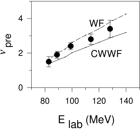
The experimental values[87] of evaporation residue cross-section are also shown in this figure.
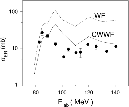
We first note that the calculated evaporation residue cross-section is very sensitive to the dissipation in the fission degree of freedom. The WF predictions are a few times (typically 2-5) larger than those obtained with the CWWF. Next we make the important observation that the CWWF predicted excitation function is much closer to the experimental values than that obtained with the WF. This observation clearly shows that the chaos-weighted factor in CWWF changes its strength in the right direction. We must take note of the fact, however, that the CWWF still considerably overestimates the ER cross-section. Since the present dynamical calculation considers only one (elongation) fission degree of freedom, it is expected that inclusion of the neck degree of freedom will increase the fission probability [162] further and hence reduce the ER cross-section. We plan to extend our work in this direction in future. We further observe that while a peak appears in the experimental excitation function at about 85 MeV, the same is shifted by 10 MeV in our calculated results. We do not have any explanation for this discrepancy except pointing out that there is no free parameter in our calculation and thus no parameter tuning has been attempted in order to fit experimental data. A similar shift has also been observed in an earlier work[159].
The structure of the evaporation residue excitation function can also reveal certain interesting features. Since the calculated values of the evaporation residue cross-section are obtained as the product of the fusion cross-section and the probability of evaporation residue formation, the initial rise of the ER cross-section with beam energy essentially reflects the steep rise of fusion cross-section in this energy region [193]. The high energy part of the ER cross section excitation function is due to charged particle emission and this part even seems to rise slowly with excitation energy[86]. The reason for that is that after the emission of some charged particles the daughter nuclei becomes less fissile and survive with higher probability. This mechanism works more successful for higher excitation energy because of the reduced role of the Coulomb barrier. This establishes the significant role of charged particle emission in the survival probability of a nucleus. An experimental finding like this is reported in Ref. [195]. At higher beam energies, the ER cross-section becomes approximately stable which results from a delicate balance between the increasing trend of the fusion cross-section and the decreasing trend of the probability of ER formation. Had the ER formation probability decreased at a rate higher than those obtained in the present calculation, the resulting ER cross-section would have decreased at higher compound nuclear excitations. In fact, such an observation was made in Ref. [87] where the ER
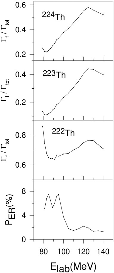
cross-section obtained from standard statistical model calculation was found to decrease very steeply beyond 100 MeV of beam energy. In order to explore this point a little further, we have calculated the excitation function of the partial width for fission. Since fission can take place at any stage during neutron (or any other light particle) evaporation, the partial widths are calculated for 222Th and 223Th as well at excitation energies reduced by the neutron separation energy after each neutron emission. The compound nuclear spin was taken as from Eq. 4.2 (section 4.1.2) while only chaos-weighted wall friction was considered for this calculation.
The calculated excitation functions of the fission partial widths are shown in Fig. 5.3. The calculated values of the ER formation probability () are also displayed in this figure. Each partial width excitation function is found to have a minimum around 90 MeV of beam energy after which it starts increasing till this trend is arrested and reversed at higher excitations. Recalling the fact that the above results on partial widths are only indicative while is obtained from a full dynamical calculation, it is of interest to note that a bump in the excitation function of also appears in the above ( 90 MeV) energy range. Subsequently, the value of drops rather sharply before it settles to a steady value at higher excitations. This feature is also complementary to that of the excitation functions of the partial widths of fission. We thus demonstrate in a schematic manner how the structure in the excitation function of the ER cross-section is related to the competition between fission and other decay channels at different stages of fission.
5.3 Summary
We have applied a theoretical model of one-body nuclear friction, namely the chaos-weighted wall friction, to a dynamical description of compound nuclear decay where fission is governed by the Langevin equation coupled with the statistical evaporation of light particles. We have used both the standard wall friction and its modified form with the chaos-weighted factor in order to calculate the prescission neutron multiplicity and evaporation residue excitation functions for the 224Th nucleus. Though the number of the prescission neutrons calculated with either wall friction or chaos-weighted wall friction are found to be very close to each other in the energy range considered, the evaporation residue cross-section is found to depend very strongly on the choice of nuclear friction. The evaporation residue cross-section calculated with the CWWF gives a much better agreement with the experimental data compared to the WF predictions. This result demonstrates that the consequences of chaos in particle motion give rise to a strong suppression of the strength of the wall friction for compact shapes of the compound nucleus which, in turn, brings theoretically calculated evaporation residue cross-sections considerably closer to the experimental values. Thus the chaos considerations may provide a plausible explanation for the shape-dependence of the strength of nuclear friction which was found [150, 159] to be necessary in order to fit experimental data.
Chapter 6 Effect of transients in nuclear fission
Induced nuclear fission had been viewed by H. A. Kramers as a diffusion process of the fission degree of freedom over the fission barrier long before the successful developments of transport theories for description of heavy ion reactions [8]. In the eighties, forty years after Kramers, Weidenmüller et al. made a detailed study of nuclear fission using the Fokker-Planck equation within the framework of this diffusion model [32]. The work of Weidenmüller et al. first revealed that it requires a certain interval of time to develop a steady probability flow at the saddle point across the fission barrier. During this time interval, also referred to as the transient time , the probability flow at the saddle point increases from zero to its stationary value. This stationary probability flow also defines the stationary fission width () and the associated fission life time (). More specifically, the fission-decay width is inhibited at its earliest times and thus at the beginning of the process, during a delay of the order of the transient time , the fission-decay width differs from its asymptotic value (), originally derived by Kramers by solving the stationary Fokker-Planck equation[8].
The transient time which arise from the relaxation of the collective degrees of freedom has significant effects on the prescission particle and multiplicities and on the future evolution of the nucleus, in particular its fission probability. The crucial quantities which govern the time evolution of the probability current across the barrier are: the excitation energy of the system, the height of the fission barrier and the nuclear friction coefficient. Depending on the values of these quantities, completely different situations may be encountered. One possibility is a slow attainment of a quasistationary regime of probability flow over the transient time . On the other extreme, the entire distribution may pass the barrier in a single swoop and the whole fission process becomes a transient[37]. These different situations are clearly not taken into account in the “statistical model” of Bohr and Wheeler, which assumes from the outset the existence of a quasistationary regime at the saddle point. In particular, when the entire distribution comes close to pass the barrier in a single swoop it is not possible to define a fission width in the usual sense. Thus the standard treatment of the cascade de-excitation and associated cooling of a compound nucleus via particle emission and fission needs to be modified accordingly.
Weidenmüller and his coworkers generalized the quasistationary approach of Kramers to a time dependent one and derived for the first time a time dependent fission width solving the Fokker-planck equation analytically as well as numerically within the framework of a simplified model. From their numerical calculations, the authors of Ref. [196] extracted the following information for the transient time, defined as the time until the fission width reaches of its asymptotic value:
| (6.1) | |||||
where is the fission-barrier height, is the nuclear temperature, is the effective oscillator frequency (harmonic oscillator osculating the nuclear potential at the first minima) at the ground state, and () is the effective reduced dissipation coefficient which rules the relaxation of the collective degrees of freedom towards thermal equilibrium. They distinguished two regimes for the motion of the collective variable in the first minimum of the potential, which is characterized by a specific value of the reduced nuclear friction coefficient : for the motion of the collective variable is underdamped while for it is overdamped. Thus a semi-quantitative estimate of the transient time was obtained and it was found to increase with decreasing values of in the underdamped case while it increases linearly with in the overdamped case. In both the cases they derived simple analytical formula for the time-dependent fission width.
The dominant role of transients on lifetime of induced fission at high excitation energies( 100 MeV) is emphasized in Ref. [196]. The detailed study and effects of transients in the case of overdamped motion can be found in Ref. [197]. In cases where the system is highly excited and the potential minimum is very shallow or non existent(no fission barrier), the entire fission process is predominantly or completely a transient phenomenon. The transient time for such cases is redefined and a simple analytical expression is given in Ref. [37]. It appears essentially as the time for the onset of the exponential growth of fluctuations i.e. the time when the system becomes globally unstable and breaks apart. The solution of Fokker-Planck equation to arrive at an analytical expression for the time-dependent fission width is significant since incorporation of this in a statistical model evaporation code is equivalent to a dynamical study of nuclear fission by Langevin or Fokker-Planck equation [198]. Due to the high computing time required by the Langein or the Fokker-Planck approaches, this equivalent procedure of using a cascade code (where fission is treated as one of the decay channels and time dependence of fission width is explicitly taken into account) is often preferred to interpret experimental data. This realization motivated improved deduction of from the analytical solution of the Fokker-Planck equation. One of the work worth mentioning is the meticulous investigation by B. Jurado et al. of the evolution of the probability distribution of the system in phase space all along its dynamical path which resulted in extracting the main features of the relaxation process towards equilibrium [199]. Characteristic features of the evolution of the amplitude of the probability distribution and the velocity profile at the fission barrier were derived. Making use of these results, they have developed an easily calculable approximation of the time dependent fission-decay width that is based on realistic physical assumptions, taking the initial conditions into account properly. This new analytical formulation of was able to reproduce rather closely the trend of the exact numerical solution in the under- as well as in the over-damped regime[200].
6.1 Experimental signatures
The tools most frequently applied to measure fission time scales are the neutron clock[65] and the gamma clock[67]. They have yielded the majority of the available information on the time interval a heavy nuclear system needs to cross the scission point. However, the mean scission time is an integral value, including the transient time, the inverse of the stationary decay rate(the statistical decay time) and an additional dynamic saddle-to-scission time. Thus it does not give direct access to the transient time that is connected to the equilibration process of the compound nucleus. The total fission or evaporation residue cross section have been used to investigate dissipation at low deformation, but they are not sufficient to determine transient effects in an unambiguous way. The challenge to observe transient effects is increased by the fact that they show up only in a restricted energy range. The calculations of Ref. [201] have shown that that fission is affected by transient effects only for excitation energies at saddle within the interval . At excitation energies below 150 MeV, the statistical decay times for fission is appreciably longer than typical dynamical time scales, making the dynamical observables rather insensitive to the transient time. This point may explain why in several experiments performed at rather low excitation energy no transient effects at all were observed[202]. In fact, the observation of transient effects requires a reaction mechanism that forms excited nuclei with an initial population in deformation space far from equilibrium and an experimental signature that is specifically sensitive to the delayed population of transition states.
In peripheral relativistic heavy-ion collisions using at 1 GeV, fission studies in inverse kinematics were carried out at GSI[203]. They studied projectile-fragmentation - fission reactions and introduced two experimental signatures to observe transient effects in fission. The total fission cross sections of projectiles at 1 GeV were studied as a function of the target mass and also the partial fission cross sections and the partial charge distributions of the fission fragments were investigated for the reaction of on target. The first signature exploited to measure transient effect was given by the partial fission cross-sections, i.e. the fission cross sections as a function of . At high excitation energies particle decay times become smaller than the transient time and the nucleus can emit particles while fission is suppressed. Therefore, for the lightest fissioning nuclei (lowest values of ) transient effects will lead to a considerable reduction of the fission probability. The second signature is based on the charge distribution of the fission fragments that result from a given fissioning element. The width of the charge distribution of the fission fragments is a measure of the saddle point temperature[203] and thus for the lower values of where the initial excitation energy is large and fission is suppressed with respect to evaporation, the nucleus will evaporate more particles on its way to fission. Therefore, transient effects will reduce the temperature of the system at saddle and consequently the width of the charge distributions[204]. These experimental observables were compared with an extended version of the abrasion-ablation Monte-Carlo code ABRABLA to deduce quantitative results on transient effects. The results demonstrated the suppression of fission at high excitation energies and thus established the importance of transients.
6.2 Transients in our model
The studies of transients as described earlier in this chapter were carried out under a number of simplifying assumptions. The potential chosen was not realistic(simplified) and the inertia and friction parameter were taken as constants so that analytical solution of the Fokker-Planck equation is possible as well as the numerical solution becomes easier. However it has been established by extensive experimental data that friction coefficient is not constant but strongly shape dependent and hence numerical study of the fission process becomes inevitable. This motivated us to use our model for friction namely the chaos-weighted wall friction in Langevin dynamics and study the effects of transients in nuclear fission in a much more realistic framework with a Yukawa plus exponential double folding potential.
In the present work, we would examine certain issues related to the time dependence of fission widths and its effect on the multiplicity of the prescission neutrons. First, we would study the effect of lowering the fission barrier on the time dependence of the rate of fission. The motivation for this study is to find the transition from a diffusive process in the presence of a fission barrier to a transient dominated picture when there is no fission barrier. We would indeed find that the diffusive nature of fission continues to some extent even for cases which have no fission barrier. The underlying physical picture that would emerge for fission in the absence of a fission barrier would be as follows. Consider an ensemble of fission trajectories which have started together sliding down the potential (with no fission barrier) towards the scission point. However, the random force acting on the trajectories will introduce a dispersion in their arrival time at the scission point. In other words, the trajectories will cross the scission point at different instants and a flow will thus be established at the scission point. However, the effect of this dispersion will be reduced when the conservative force becomes much stronger than the random force. This would happen at very large angular momentum of the fissioning nucleus due to the strong centrifugal force. Therefore, the single swoop picture for fission becomes more appropriate at very large values of spin of the nucleus. We would establish the above scenario in the first part of our work.
It is already stated that the study of fission dynamics using Langevin or Fokker-Planck equation requires huge amount of computation time and can be avoided by adopting an alternative and easier approach which is to perform a statistical model calculation by modifying a cascade code in which fission is treated as one of the decay channels and the time dependence of the fission width is explicitly taken into account [198]. In such calculations, the input fission widths and the transient times are usually taken from the analytical expressions deduced from the solution of the Fokker-Planck equation under simplifying assumptions [8, 32, 59, 200]. These analytical expressions for were all obtained under the approximation of constant, shape-independent nuclear friction. However, since friction was shown to be strongly shape dependent by extensive experimental work and theoretical analysis, numerical solution of the dynamical equation is essential. In our work, the fission widths will be obtained numerically by solving the Langevin equation using the chaos-weighted wall friction[174] (as described in chapter 3) and the transient time will be obtained by fitting the numerically calculated fission widths with an analytical expression. Thus the expression for to be used in the statistical calculation has inputs from the numerically solved Langevin dynamics and hence is a much realistic description of the actual process. In the next part of our work, we would perform such statistical model calculations for prescission neutron multiplicity using the time dependent fission widths as well as the single swoop description of fission. This would be done with the aim of finding how well the statistical model calculations with and without the single swoop assumption agree with each other. We would subsequently calculate the prescission neutron multiplicity in a dynamical model of fission and compare the results with those obtained from the statistical calculations with time dependent fission widths. Though one would expect the results from the statistical and the dynamical calculations to be the same, there could be some differences and we would ascertain the magnitude of such differences from our calculation.
As we have shown in chapter 4, the prescission neutron multiplicity and fission probability calculated from Langevin dynamics using the chaos-weighted wall friction were found to agree fairly well with the experimental data for a number of heavy compound nuclei () over a wide range of excitation energies [158]. This observation as well as the fact that CWWF does not contain any free parameter to fit experimental data motivated us to use this modified form of one-body friction to pursue our study of transients in this work. In the 3rd chapter, a systematic study of fission widths using this friction is already reported. That study was confined to cases with fission barriers whereas we would concentrate upon fission in the absence of a barrier in the present chapter. The details of our model including the nuclear shape, potential, inertia and friction is given in the 2nd chapter. The next section will contain the numerical results of our study while the last section will present a summary of this chapter.
6.3 Results
6.3.1 Fission widths from Langevin equation
The time-dependent behaviour of fission widths under different physical conditions is being studied here using the Langevin equation. Starting with a given total excitation energy () and angular momentum () of the compound nucleus, the energy conservation in the following form,
| (6.2) |
gives the intrinsic excitation energy and the corresponding nuclear temperature at each integration step. A Langevin trajectory will be considered as having undergone fission if it reaches the scission point () in the course of its time evolution. The calculations are repeated for a large number (typically 100 000 or more) of trajectories and the number of fission events is recorded as a function of time. Subsequently the time dependent fission rates can be easily evaluated as described in chapter 3.
We have chosen the 200Pb compound nucleus for our study which has been experimentally formed at different excitation energies in a number of heavy ion induced fusion reactions [62, 187, 188]. The results which will be described in this section is reported in Ref. [205]. Fig. 6.1 shows the calculated time dependent fission widths at different spins of the compound nucleus for a given temperature. A number of interesting observations can be made from this figure. The time dependence of the fission width of the compound nucleus with a spin of 40 (and with a fission barrier) is typical
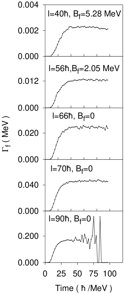
of a diffusive flow across the fission barrier which has been studied extensively in chapter 3[174]. The fission width is found to remain practically zero till a certain interval of time () which essentially corresponds to the interval after which the fission trajectories start arriving at the scission point. The fission width subsequently increases with time till it reaches its stationary value (). The following parametric form will be used for the time dependent fission width in order to enable us to use it in our later calculations,
| (6.3) |
where is a measure of the transient time after which the stationary flow is established and is the step function. The intervals and are obtained by fitting the calculated fission widths with the above expression.
It is observed from Fig. 6.1 that the nature of the time dependence of the fission width remains almost same even though the fission barrier decreases and subsequently vanishes with increasing spin. At very large values of spin, however, fluctuations appear at the later stages of time evolution. These fluctuations are statistical in nature because the number of nuclei which have not yet undergone fission decreases very fast with increasing time for higher values of spin and therefore introduces large statistical errors in the measured numbers. The magnitude of the fluctuations can thus be reduced by considering a larger number of fission trajectories. In our calculation, we have taken particular care by using larger ensembles at higher values of nuclear spin in order to enable us to check whether a stationary value of the fission width is attained at all.
The above observation is of particular interest since it shows that the diffusive nature of fission persists even for cases which have no fission barrier. This diffusive nature is a consequence of the random force acting on the fission trajectories as we have discussed earlier. As a compound nucleus is formed having no potential pocket in the fission channel, it starts rolling down the potential towards the scission point. However, the random force acting on these fission trajectories introduces a spread in their arrival time at the scission point. The spread in the arrival time of the fission trajectories gives rise to a finite fission width as we find in Fig. 6.1.
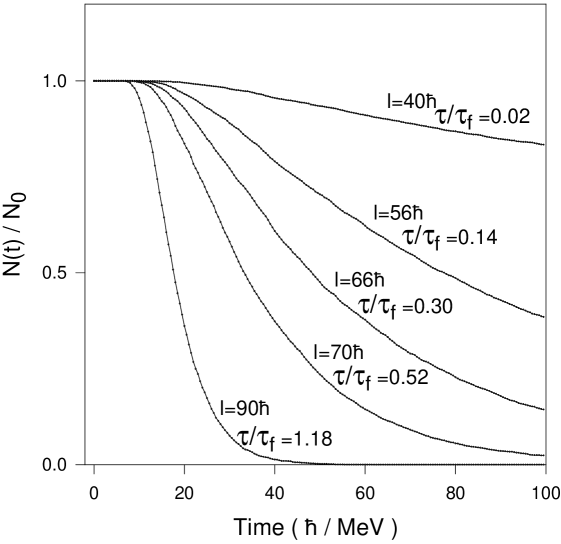
In order to further investigate the above diffusive nature of fission, the fraction of the number of compound nuclei which have survived fission is shown as a function of time in Fig. 6.2. The same compound nuclei as in Fig. 6.1 has been considered for this figure. Here we find a gradual shift in the decay rate with increasing spin of the compound nucleus. Specifically, the exponential decay of the number of compound nuclei having a fission barrier (with spins 40 and 56) is found to continue for those without fission barriers (with spins 66, 70 and 90). Subsequently the fraction of the surviving compound nuclei have been calculated from the Langevin dynamics by switching off the random force. Fig. 6.3 shows this decay in which all the nuclei have the same life time which is simply the swooping down time () from the initial to the scission configuration. The spread in the life time of the trajectories around this value when the random force is switched on can also be seen in this figure. It may also be noted that for very large values of the compound nuclear spin, the decay is very fast and consequently, the above spread is very small. For such cases, fission is dominated by the transients and can be approximated by a single swoop process.
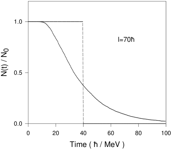
The relevance of the different time scales in order to distinguish between the roles of stationary flow and transients in fission will now be investigated. When the fission life time () is much longer than the transient time , most of the fission events take place after the establishment of a stationary flow. Evidently, this holds for nuclei with a barrier in the fission channel. However, it is also possible to have for cases which have no fission barrier.
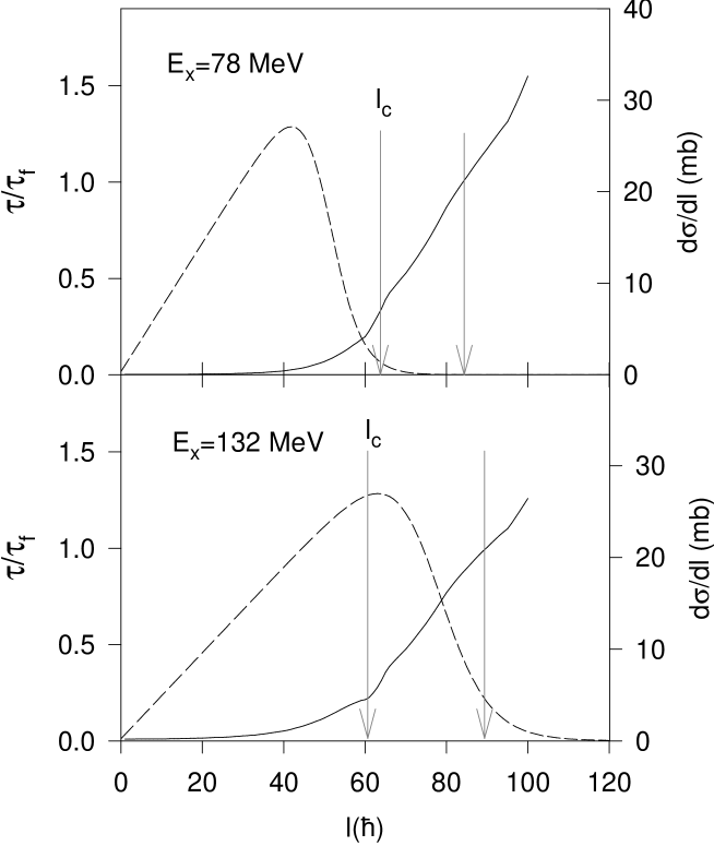
This is illustrated in fig. 6.4 where the ratio is plotted as a function of the spin of the nucleus. Beyond the critical angular momentum at which the fission barrier vanishes, we find a window of angular momentum where is indeed greater than . This window represents the transition region over which the fission dynamics changes from a steady flow to transients. Fission becomes transient dominated for spin values at which . A single swoop description of fission can be applied for such cases. However, a single swoop picture would be rather inaccurate in the transition region where a steady flow still persists. In the next subsection, the consequences of using the single swoop description of fission in statistical model calculations in terms of the multiplicities of prescission neutrons will be explored. It would be of interest for our later discussions to locate the transition region with reference to the spin distributions of the compound nuclei formed in heavy ion induced fusion reactions. The spin distribution of the compound nucleus 200Pb obtained in the fusion of +181Ta at two excitation energies is therefore plotted. It is observed that the transition region lies beyond the range of the spin distribution when the compound nucleus is excited to 78 MeV, whereas it is well within the range of the spin values populated at an excitation of 132 MeV. One would thus expect that the number of prescisssion neutrons would be affected more at higher excitation energies when the single swoop picture is used in the transition region.
6.3.2 Prescission neutrons from dynamical and statistical model calculation
A comparison of the prescission neutron multiplicity from the Langevin dynamics of fission as well as from a statistical model calculation (where time-dependent fission widths will be used) is studied in details in this section. The details of the dynamical model along with statistical evaporation of neutron and giant dipole is described in the 4th chapter. The same procedure is followed in the present calculation. A Langevin trajectory will be considered as undergone fission if it reaches the scission point in course of its time evolution. Alternately it will be counted as an evaporation residue event if the intrinsic excitation energy becomes smaller than either the fission barrier or the binding energy of a neutron. The calculation proceeds until the compound nucleus undergoes fission or ends up as an evaporation residue. The number of emitted neutrons and photons is recorded for each fission event. This calculation is repeated for a large number of Langevin trajectories and the average number of neutrons emitted in the fission events will give the required prescission neutron multiplicity.
The statistical model calculation of prescission neutron emission proceeds in a similar manner where a time-dependent fission width is used to decide whether the compound nucleus undergoes fission in each interval of time evolution. The intrinsic excitation energy at each step is given by the total excitation energy minus the rotational energy since no kinetic energy is associated with the fission degree of freedom in the statistical model and the compound nucleus is assumed to be in its ground state configuration (zero potential energy). Two prescriptions for the time-dependent fission widths will be used in our calculation. In the first one, we shall use the parametric form of the width given by Eq. 6.3 for all spin values including those for which there is no fission barrier. The parameters , and are obtained by fitting the numerically calculated time-dependent widths. In the other statistical model calculation, the above parametric form will be used only for those spin values which have fission barriers. For higher spin values for which there is no fission barrier including those in the transition region, the swooping down picture will be applied. For these cases, the swooping down time is evaluated numerically as explained earlier. In this statistical model calculation, neutron and evaporation can take place during this period while the nucleus will be considered as undergone fission at the end of this interval.
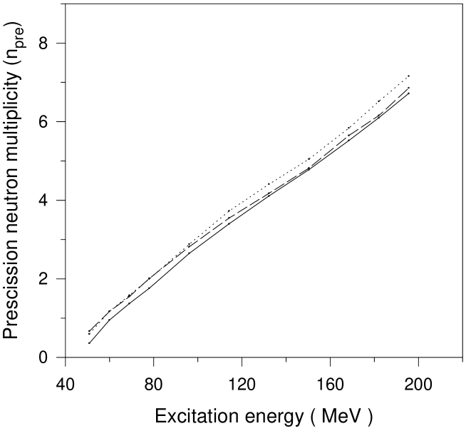
Fig. 6.5 shows the calculated prescission neutron multiplicity at different excitation energies of the compound nucleus 200Pb formed in the 19F + 181Ta reaction. Results shown in this figure are obtained from the dynamical and statistical model calculations which are continued for a period of 300. This time period is not sufficient for all the nuclei in the ensemble either to reach the fission fate or to become evaporation residues. Pushing the Langevin calculation much beyond the above time period becomes prohibitive in terms of computer time. The above time duration is however much longer than the transient times and hence are adequate for our purpose of comparing the dynamical and statistical results.
It is observed from Fig. 6.5 that the neutron multiplicity calculated from the statistical model using the time-dependent fission widths with and without swooping down assumption are almost same at lower excitation energies though they differ marginally at higher excitation energies. Such a difference was anticipated in the earlier subsection since the swooping down assumption is invoked more frequently for compound nuclei at high excitation energies which are mostly formed with large values of spin and consequently with no fission barrier.
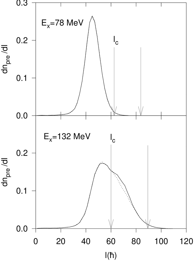
In order to explore this point further, the differential neutron multiplicities are obtained from the statistical model calculations with as well as without the single swoop description and are shown in Fig. 6.6. The two calculated distributions at an excitation energy of 132 MeV are found to be different beyond though they merge again at the higher end of the transition region. This difference essentially reflects the approximate nature of the single swoop description in the transition region. However, the magnitude of this difference is found to be rather small ( a few ). At a lower excitation of 78 MeV, the two distributions are almost identical as one would expect since they have very little overlap with the transition region. The significance of the above observations is of interest since it shows that for compound nuclei without a fission barrier, considering a sharp valued life time (the swooping down time ) instead of a life time with a dispersion does not make any appreciable effect in the number of emitted neutrons before fission. It is next observed in Fig. 6.5 that the neutron multiplicity from the statistical (both calculations) and dynamical models are also very close to each other though the statistical models marginally overestimate the neutron multiplicity compared to the dynamical model. A possible explanation for this observation would be the fact that the compound nuclear temperature in the statistical model is higher than that in the dynamical model since a part of the total excitation energy is locked up as kinetic energy of the fission mode in the dynamical model. This reduces the intrinsic excitation energy and hence the temperature in the dynamical model resulting in a smaller number of evaporated neutrons.
It is already mentioned that a full dynamical calculation can take an extremely long computer time particularly for those compound nuclei whose fission probability is small. Hence the combined dynamical and statistical model, first proposed by Mavlitov et al. is followed [178], in order to perform a full calculation. This approach has been described in details in the previous chapter. In this model, the time evolution of a compound nucleus is followed according to the Langevin equations for a sufficiently long period (during which a steady flow across the fission barrier is established) and then switch over to a statistical model description after the fission process reaches the stationary regime. It is possible to continue this calculation for a sufficiently long time such that every compound nucleus can be accounted for either as an evaporation residue or having undergone fission.
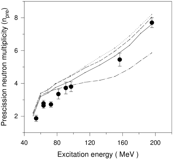
The prescission neutron multiplicity calculated with the above combined dynamical and statistical model is shown in Fig. 6.7 along with the full statistical model calculations. The statistical model calculations are made with as well as without the swooping down assumption in the time-dependence of the fission widths. The experimental values are also shown in this figure. The observations made in this figure are similar to those in Fig. 6.5, namely, the statistical calculations slightly overestimate the neutron multiplicity compared to the dynamical (plus statistical) calculation. However, the statistical and dynamical results are quite close to each other and are also close to the experimental values. This result therefore shows that the statistical calculation with time-dependent fission width can represent the dynamical calculation with reasonable accuracy. The results of a statistical calculation is also shown in this figure where the fission widths are assumed to be independent of time and are given by their stationary values. This calculation substantially underestimates the neutron multiplicity and illustrates the importance of transients at higher excitation energies.
6.4 Summary
We have presented in the above a numerical study of the transients in the fission of highly excited nuclei and their effect on the number of neutrons emitted prior to fission. To this end, we first investigated the time-dependence of fission widths using the Langevin dynamics of fission. We have shown that the fission width reaches a stationary value after a transient period even for those nuclei which have no fission barrier. We have discussed the role of the random force acting on the fission trajectories in introducing a dispersion in their arrival time at the scission point and thereby giving rise to a finite rate of fission for such cases. We have also shown that this stationary fission rate for very large values of spin of the nucleus loses significance since the stationary fission life time itself becomes much smaller than the transient time for such cases. Therefore, fission of nuclei rotating with a large angular momentum can be considered to proceed in a single swoop. Our study demonstrates a gradual transition from a diffusive to a single swoop picture of fission with increasing spin of the compound nucleus.
We have subsequently examined the effect of the transients on the multiplicity of the prescission neutrons emitted in heavy ion induced fusion-fission reactions. We used both the diffusive description and the swooping down picture separately in statistical model calculations and found close agreement between the two calculated neutron numbers at low excitation energies whereas they differed marginally at higher excitations. It was also shown that the differential neutron multiplicities calculated with and without the single swoop assumption differ only in the transition region though the magnitude of the difference is small. We therefore conclude that the single swoop description of fission can be used in statistical model calculations without making any significant error in the final observables.
We finally compared the number of neutrons calculated from a dynamical model with that obtained from a statistical model in which time-dependent fission widths are used. We found that the statistical model marginally overestimates the neutron numbers than those from the dynamical calculation. We explained this difference in terms of the temperature which is lower in the dynamical model than the statistical calculation. The temperature turns out to be smaller in the dynamical model because the excitation energy is shared between the collective fission mode and the thermal mode in the dynamical calculation in contrast to the statistical calculation where the full excitation energy is assumed to be available in the thermal mode. However, in most of the fission events in the dynamical calculation, the kinetic energy builds up to values which are a little above the fission barrier before it proceeds to fission. Since the values of the fission barrier (typically a few MeV or less) are much smaller than the excitation energies (a few tens of MeV or more) considered here, the temperature differences between the statistical and dynamical calculations remain small for most of the cases. Consequently the difference between the prescission neutron multiplicities calculated from the dynamical and statistical models become small, as we have observed in our calculation.
Chapter 7 Summary, discussions and future outlook
7.1 Summary and discussions
A detailed study of fission dynamics of highly excited nuclei formed in heavy-ion collisions is presented in this thesis with a view to extract knowledge about the dissipative properties of hot fissioning nuclei. Chaos-weighted wall friction(CWWF) which is a microscopic model of nuclear friction, is incorporated in a Langevin dynamical model, and different observables namely prescission neutron multiplicity, fission probability and evaporation residue cross-sections are calculated. CWWF takes into account the nonintegrabilty of single particle motion in the nucleus and it resulted in a strong suppression of friction strength for near spherical shapes of the nucleus. A general introduction to the subject and application of Langevin dynamics in fission with description of different input parameters are given in chapter 1 and 2 respectively.
In chapter 3 a systematic study of the fission widths is made for different excitation energies and spins of a compound nucleus, using both CWWF and WF in the Langevin equation. The fission widths calculated with CWWF turned out to be about twice the widths calculated with the normal wall friction(WF). A parametric representation of the calculated fission widths in terms of the temperature and spin of the compound nucleus was made so that they can be used in subsequent statistical model calculation of the decay of a highly excited compound nucleus which requires dynamically calculated fission widths as inputs. The substantial enhancement in the fission widths with CWWF was expected to influence fission probability and neutron multiplicity and this motivated the use of these parameterized widths in the next part of our work.
In chapter 4 of this thesis, the chaos-weighted wall friction is applied to a combined dynamical plus statistical description of compound nuclear decay where fission is governed by the Langevin equation coupled with statistical evaporation of light particles and photons. The calculation was done using both CWWF and WF and the results show that both the prescission neutron multiplicity as well as the fission probability calculated with the chaos-weighted wall friction for the compound nuclei 178W, 188Pt, 200Pb, 213Fr, and 224Th agree much better with the experimental data compared to the predictions of the normal wall friction. The separate contributions of presaddle and postsaddle neutrons at different excitation energies were investigated in order to gain further insight into the dynamics of fission. The postsaddle neutron multiplicities calculated with the CWWF and WF are almost same for all the compound nuclei over the range of excitation energies considered. This is due to the fact that the number of post saddle neutrons depend on the strength of friction between saddle and scission, and CWWF and WF are indeed close to each other in this regime of large deformation. The wall friction predictions for the presaddle contribution to neutron multiplicity are consistently higher than those from CWWF at higher excitation energies and this gives rise to the enhancement of the WF prediction for total prescission neutron multiplicity as compared to that from CWWF predictions. Since CWWF predicted neutron multiplicities better agree with the experimental values for all the above nuclei, we conclude that the chaos-weighted wall friction provides the right kind of friction to describe the presaddle dynamics of nuclear fission.
It was also noted that the majority of the prescission neutrons are emitted in the postsaddle stage for a very heavy nucleus like 251Es. The chaos-weighted wall friction, however, cannot produce enough neutrons to match the experimental prescission multiplicities for such a nucleus. It is, therefore, possible that in the postsaddle region, either the fission dynamics gets considerably slowed down or the neutrons are more easily emitted. The neutron widths from a highly deformed nucleus could be quite different from that of the equilibrated near-spherical nucleus which we use in our calculation. Also, dynamical effects, like inclusion of the neck degree of freedom in the Langevin equation can influence the time scale of post saddle dynamics and hence the number of neutrons.
In chapter 5, we have used the evaporation residue cross-sections as probe for nuclear dissipation. We have used both the standard wall friction and its modified form with the chaos-weighted factor in order to calculate the prescission neutron multiplicity and evaporation residue excitation functions for the 224Th nucleus. It is found that WF and CWWF predictions for neutron multiplicity are very close to each other in the energy range considered, and hence is not a sensitive probe for nuclear friction in this energy regime. It is further noted from the results that the calculated evaporation residue cross section is very sensitive to the dissipation in the fission degree of freedom, the WF predictions being few times (typically 2-5) larger than those obtained with the CWWF. The most important observation is that the CWWF predicted excitation function is much closer to the experimental values than that obtained with the wall friction, which clearly shows that the chaos-weighted factor in CWWF changes its strength in the right direction. Thus the chaos considerations may provide a plausible explanation for the shape-dependence of the strength of nuclear friction which was found [150, 159] to be necessary in order to fit experimental data.
In chapter 6, a numerical study of the transients in the fission of highly excited nuclei was presented using our dissipative dynamical model of nuclear fission and also the effect of the transients on the number of prescission neutrons was investigated. The detailed study of the time-dependent fission widths demonstrated a gradual transition from a diffusive to a single swoop picture of fission with increasing spin of the compound nucleus. It was found that the fission width reaches a stationary value after a transient period even for those nuclei which have no fission barrier. The stationary fission life time for such nuclei is much smaller than the transient time and hence fission can be considered to proceed in a single swoop for nuclei rotating with large angular momentum. For nuclei with no fission barrier, the diffusive picture and the swooping down assumption were used separately in statistical model calculations and close agreement was found on the calculated prescission neutron numbers which justified the use of swooping down description of fission in statistical model calculation without making any significant error in the final observables.
Finally, it was noted that statistical model calculation with time dependent fission widths marginally overestimates the prescission neutron multiplicity than a dynamical calculation. This is mainly because the intrinsic excitation energy turns out to be smaller in the dynamical model since total excitation energy is shared between collective and thermal degrees whereas in statistical description the full excitation energy is available in the thermal mode. The number of neutrons emitted depends sensitively on the compound nuclear temperature which is directly proportional to the intrinsic excitation energy and thus the dynamical model calculation ends up with a marginally smaller number of neutrons. It is to be noted that this temperature difference between the two types of calculation is small for most cases and hence the difference between the neutron numbers as observed from the calculations is marginal and thus statistical model calculation with time dependent fission widths can represent a dynamical model calculation with reasonable accuracy.
7.2 Future Outlook
The dynamical model of fission of hot nuclei using the chaos weighted wall friction can be extended to include the asymmetry degree of freedom in the dynamics in order to study the fission fragment mass energy distributions. The available experimental data of the prescission neutron multiplicities as a function of the fragment mass asymmetry and kinetic energy can be compared with the results of this dynamical model which includes asymmetry parameter as a collective coordinate. The comparison of such exclusive experimental data with the theoretical results is in fact a crucial test for the stochastic approach to fission dynamics based on the Langevin equations. This will also help in analyzing and elucidating correlations between the prescission neutron multiplicities and fission fragment mass energy distribution and to study the fission fragment angular anisotropy. It is claimed in [65] that fission fragment angular anisotropy is strongly affected by evaporation of presaddle neutrons and hence is a strong probe of dissipation, in particular for compact configurations. Three dimensional Langevin calculations of the fission fragment mass energy distributions have been carried out[151, 152] using wall friction with a adjustable reduction coefficient. Our model of nuclear friction (CWWF) should be used for such three-dimensional dynamical calculations and analysis of the relevant experimental data. This calculation will be of great significance since it can predict the production cross section of exotic nuclei as asymmetric fission fragments. The chance of formation of exotic nuclei by this method will depend sensitively on nuclear dissipation and CWWF is expected to play a significant role. The production cross-section of fission fragments predicted by the fission dynamics calculation is also expected to have significant bearing on transmutation of nuclear waste.
The neck degree of freedom designated by the coordinate in our shape parametrization, will be included in our dynamical model in near future in order to compare the results of the already reported one dimensional calculation with the two dimensional one. Fission rates obtained from the two dimensional calculation is expected to improve upon that of the one dimension though the difference will not be very significant. On the whole, the effect of incorporation of this additional collective coordinate in the dynamical model is expected to influence the prescission neutron multiplicity and fission probability in a favourable direction. The inclusion of an additional degree of freedom will increase the accuracy of our dynamical model and hence will be a better test of our model of friction. The production cross section of evaporation residues which can be better predicted from this multi-dimensional fission dynamics model will help in search of superheavy elements formed as evaporation residues.
It was concluded from the analysis of our results of postsaddle, presaddle and total prescission neutrons that chaos weighted wall formula is the right kind of friction to describe the presaddle dynamics of a hot rotating nucleus. It was also noted that for a heavy nucleus like , most of the prescission neutrons are contributed by the post saddle ones and the calculated number using CWWF number falls short of the experimental value by a considerable margin. In fact, it was seen that in order to match experimental data, the empirical friction of Frobrich et al. needs to be much stronger in the large deformation region(post saddle part) than that given by the chaos weighted wall formula. However, there is no physical justification of increasing the strength of the nuclear dissipation in the post saddle region beyond that of the wall friction. Instead, we feel that the mechanism of neutron emission in the postsaddle stage requires a closer scrutiny essentially because the nucleus becomes strongly deformed beyond the saddle point. The neutron decay width of such a strongly deformed nucleus could be quite different from that of the equilibrated near-spherical nucleus which we use in our calculation. In particular, the neutron-to-proton ratio is expected to be higher in the neck region than that in the nuclear bulk and this can cause more neutrons to be emitted. Further, dynamical effects such as inclusion of the neck degree of freedom in the Langevin equation can influence the time scale of the postsaddle dynamics and hence the number of emitted neutrons. Such possibilities should be examined in future for a better understanding of the postsaddle dynamics of nuclear fission.
In our model we have not used any explicit temperature dependence of the dissipation coefficient. However, the necessity for clarifying the role of the deformation and the temperature dependence is exemplified in a recent paper by Dioszegi et al. [159] who were able to reproduce their data with a modified statistical model by applying either a strong temperature dependent friction form factor or with a deformation dependent form factor. A temperature dependence of nuclear friction is expected from general considerations since large phase space becomes accessible for particle-hole excitations at higher temperature. In fact in a microscopic calculation using linear response theory Hofmann et al. have obtained a temperature dependence of the form of . The role of the temperature dependence of the friction factor predicted by microscopic theory is still to be clarified by using it in Langevin calculations and confronting the results with experimental data. Our model can be extended to include a form factor in the friction coefficient which will represent the temperature dependence in order to examine its effect on the final observables. Questions such as whether both shape and temperature dependence should exist simultaneously or either one of them is sufficient should be addressed in future. Investigations regarding the nature of dependence on temperature is also to be carried out in order to arrive at a conclusive picture of the friction form factor with respect to its deformation and temperature dependence.
Quantal corrections are expected to modify the fission rates from classical Langevin results up to quite high temperatures. A fission rate calculated with an influence functional path integral technique gives a enhancement as compared to a Kramers rate for fission of at a temperature of 1.57MeV[206]. The inclusion of quantum effects like the shell and the pairing correlations on the potential energy landscape is expected to alter the barrier height which in turn will influence the fission rates and the fragment mass distributions as seen in Ref. [207]. At lower temperatures, e.g. when dealing with Langevin models for superheavy element formation, quantum effects are more important.
It has already been discussed in chapter 1 (section 1.2.3) that the Langevin equation needs to be generalized to allow for finite memory effects when the time scale of the fission degree of freedom becomes comparable to that of the intrinsic degrees of freedom. Thus one has to deal with a non-Markovian process when the collective motion is faster than it is assumed in our dissipative dynamical model. The chaos weighted wall friction can be extended in future to include the memory effects in order to examine its influence on the final observables. It is shown in a paper by Kolomietz et al. [208] that the elastic forces produced by the memory integral in the friction kernel lead to a significant delay for the descent of the nucleus from the barrier. Numerical calculations for the nucleus show that due to memory effect the saddle-to scission time grows by a factor of about 3 with respect to the corresponding saddle-to -scission time obtained in liquid drop model calculations with friction forces[208]. This observation implies that incorporation of the memory effects in our calculation may increase the saddle to scission time and in turn the total prescission neutron multiplicity. In fact this effect can account for the empirical need of large increase in the strength of friction in the post saddle region. Thus the non Markovian dynamics may be a possible explanation for the extra neutrons in the post saddle region.
The study of fission dynamics using the concept of “Mean First Passage Time”(MFPT) has invoked interest in recent times[209, 210, 211]. This time interval represents the average time it takes for the system to start at the potential minimum and to make its motion all the way out to scission. It included relaxation processes around the first minimum as well as the sliding down from saddle to scission. The concept of the “transient effect” is examined with respect to MFPT in [212, 213]. Our dissipative dynamical model of fission can be used to investigate this concept and its dependence on initial conditions. A comparative study of MFPT with the concept of transient time is to be made to reach at a more definite conclusion. In Ref. [214], the concept of “Mean Last Passage Time” (MLPT) is proposed for the fission rate defined at the saddle point and it is concluded that this is a better concept than that of the mean first passage time(MFPT) since a dynamical effect of descent from the saddle point to the scission point has been induced in the MLPT. This idea can be checked using our dissipative dynamical model.
In Ref. [215], one-dimensional Langevin simulations are performed to emphasize the strong sensitivity of fission transients to the assumed initial shape distribution of the compound nuclei. Fission delays or transient fission suppressions are found if the compound nucleus is initially spherical or near spherical, whereas a moderate initial fissionlike deformation can reduce the magnitude of this suppression (transient fission enhancement). It is argued that the initial conditions are determined by the fusion dynamics and thus fission transients are dependent on the entrance channel. The nature of the transients may change from suppression to an enhancement as the entrance-channel changes from asymmetric to symmetric. Transient fission will only be important when there is strong competition from evaporation of light particles and thus calculations which invoke fission delays (transient effects) to explain the large number of prescission neutrons measured in experiments should be reexamined in the light of these considerations and our dissipative dynamical model of fission can be used for this purpose.
In this work we have considered only those systems where fission follows the formation of an equilibrated compound system and the process is called fusion-fission. In our model, we have not taken into account any delay effects in the formation phase i.e., the previous pre-equilibrium stage is not considered explicitly. This assumption is valid as long as the decay time of the system is much longer than the equilibration time. However, at sufficiently high excitation energies when the transient time is comparable to or even greater than the stationary fission life time, quasi-fission or fast-fission process needs to be considered. The presence of quasi-fission process inhibits heavy element formation and thus experimental studies of this process is crucial for the search of superheavy elemnts[216, 217]. There is an increasing amount of data in which contributions of fast-fission or quasi-fission are identified; i.e. there is a need for modelling these processes.
In our model, though we calculate the number of prescission
protons, alphas and GDR ’s, we do not compare them
with experimental data because these numbers are rather small
with large statistical uncertainties in the present work. In
order to obtain the energy spectrum of the multiplicity
with a reasonable statistical accuracy, in particular, it is
necessary to perform computation using a much larger ensemble of
trajectories than the one used in the calculation presented in
this thesis. This puts a severe demand on computer time making
such computations impractical at present. However, an
alternative approach would be to make use of the time-dependent
fission widths in a full statistical calculation of the
compound-nucleus decay. This calculation would be much faster
than the present Langevin dynamical model calculation though the
time-dependent fission widths would be required as input to this
statistical model calculation. The results of the calculation
are to be folded with the appropriate detector response function
so that the calculated numbers can be compared to the experimental
data. We plan to perform such calculations in future.
Experimental scenario: The majority of the experimental approaches dedicated to the study of nuclear dissipation are based on nucleus-nucleus collisions at energies that range from 5 MeV to about 100 MeV. Among the experimental observables studied in this type of reactions the most common are the particle[65] and the -ray[67] multiplicities, the angular, mass and charge distributions of the fission fragments[218], and the fission and evaporation-residue cross sections. Except for the fission and evaporation-residue cross sections, all these observables give information on dissipation on the whole path from ground-state deformation to scission, but they do not allow exploring the deformation range from the ground state to the saddle point independently. Also, fusion-fission and quasi-fission reactions, which are mostly used, induce initial composite systems with large deformation, and therefore they do not offer suitable conditions for extracting the relevant information at small deformation. Contrary to fusion-fission and quasi-fission reactions, antiproton annihilation experiments[219, 220, 221, 222], very peripheral transfer reactions[223] and spallation reactions[204] lead to fissioning nuclei with small deformation and small angular momentum, simplifying the theoretical description considerably. Fission induced by heavy ion collisions at relativistic energies offers ideal conditions for investigating dissipation at small deformation [224]. Two new experimental signatures, namely the partial fission cross sections and the partial widths of the fission fragment charge distributions are introduced by these peripheral heavy-ion collisions[203], in order to observe transient effects in fission. These observations exploit the influence of the excitation energy on the fission probability and on the fluctuations of the mass-asymmetry degree of freedom. They are based on the particle-emission clock; however the emission of particles is translated into a reduction of excitation energy before the system passes the fission barrier. These new signatures, being sensitive to the dissipation at small deformation, is expected to give new insights into still open questions on the strength of the nuclear dissipation coefficient and its variation with deformation and temperature. These investigations are planned to be extended to projectiles between uranium and lead in order to separately vary fissility and induced energy by using secondary beams, presently available at GSI. Further progress in this field is expected when advanced installations, e.g, in the planned GSI or RIA future projects, will become available. They will allow for more sophisticated fission studies by extending the isospin range of available secondary beams and by adding new capabilities for mass-identification and light-particle-detection, aiming for kinematically complete experiments with a measure of excitation energy in individual events.
Chaos-weighted wall friction, which is the friction model used in this thesis does not have any adjustable parameter and has the same order of magnitude for low deformation as the empirical frictions which have successfully reproduced experimental data for different observables[85, 179]. In fact CWWF is the only model of deformation dependent friction derived from physical considerations which is closest to the phenomenological frictions of Fröbrich for compact shapes [225]. However, CWWF does not increase strongly for large deformations as required by the phenomenological friction[85] in order to match the prescission neutron multiplicity data for heavy systems like with a long saddle to scission path. Therefore CWWF should be applied to wider variety of systems and for different types of observables so that distinction between different models could be made more confidently in order to reach at a better picture. A systematic analysis and explanation of all the available experimental data should be attempted using CWWF in a multi-dimensional Langevin dynamical model. This will be a crucial test for our theoretical model of friction and will help to reach at a definite conclusion regarding the friction form factor with respect to its deformation (and temperature) dependence, and finally to arrive at an unified picture for fission of hot nuclei.
Appendix A
Evaluation of the nuclear potential
The potential energy is obtained from the finite-range liquid drop model, where we calculate the generalized nuclear energy by double folding the uniform density within the nuclear surface with a Yukawa-plus-exponential potential. The six dimensional double folding integral for evaluation of the potential is as follows:
| (A.1) |
where and gives the nuclear density and potential respectively. The above integral is reduced to that of lower dimensions by the method of Fourier transform. The Fourier transform in space of the charge densities and the potential are given by the following relations.
Substituting these fourier transforms in Eq. (A.1), and using the following identities,
and exploiting the properties of the delta function, the six dimensional integral is reduced to the following three dimensional integral.
| (A.2) |
Since the charge distribution is symmetric i.e., , it can be shown that and hence the integration takes the form
| (A.3) |
where the inverse Fourier transform relations,
and similarly for are used. If potential is of the
coulomb form i.e., , then it can shown using
contour integration that .
If the potential takes the exponential form i.e., , then
. For
Yukawa type of potential, i.e., ,
.
is evaluated in cylindrical
coordinate system. Due to axial symmetry in ,
will also have axial symmetry in space.
Assuming to lie in plane, it can be shown that
. Hence in
cylindrical coordinate system,
| (A.4) |
For uniform density, = constant within the defined surface.
where is the zeroth order Bessel function. Using the above result,
| (A.5) |
where
| (A.6) |
and
| (A.7) |
is calculated for to , where , and using these values of , is calculated for a wide range of of ranging from to (). The integral is evaluated for different values and the required values are extracted later by interpolating from the table. The function is thus required to be computed only once and can be used as a standard input for any subsequent double folding calculation. These values are used to evaluate in Eq. (A.5). The integral in Eq. (A.2) is finally evaluated in spherical polar coordinates. The final form of Eq. (A.2) is given by
| (A.8) |
where . The integration is done by dividing the range in two parts i.e, from to and to . The upper cut-off is chosen after ensuring a very good convergence of the integral. Since the integrand for lower values of is very oscillating, the integration here is done with very small step size, while for the second part integration is performed with a bigger step size. The stability of the potential calculation by this method is of the order of 1 in .
Appendix B
Generation of random numbers
Random number generation following a particular distribution occurs repeatedly at different stages of our calculation. The solution of Langevin equation for fission dynamics requires the generation of Gaussian distributed random number at each step of time evolution. Choosing of initial coordinates, momenta and spin of the compound nucleus also required the generation of random numbers following particular type of distribution function.
The emission of particles during the fission process as well as the energy of the emitted particles is decided by Monte-Carlo selection where random numbers are required to be generated following uniform probability distribution. The method for generation of random numbers following a particular distribution function is described here.
If the numbers , are the values of one and the same random quantity under independent trials with recurrent conditions following a particular distribution law, then the sequence of random numbers is called a random sequence with that particular distribution. To generate random numbers by computers, it is convenient to consider the sequence of random numbers uniformly distributed on the unit interval The probability of generating a number between and , denoted by , for a sequence of random numbers with a uniform and normalised () probability distribution, is given by
| (B.1) | |||||
If the random sequence is uniformly distributed on the interval , then the linear transformation
| (B.2) |
(A and B are given numbers) reduces to the random sequence
uniformly distributed on the interval .
Now if we generate a uniform deviate and then take some
prescribed function of it, say , the probability
distribution of , denoted by is determined by the
fundamental transformation law of probabilities, which is simply
| (B.3) |
For a uniform deviate for . Hence
| (B.4) |
Having a random sequence uniformly distributed on the interval , we can construct a random sequence with a specified distribution, say one with for some positive function whose integral is 1, using the above transformation method. We need to solve the equation
| (B.5) |
to get y. The solution is
| (B.6) |
i.e., indefinite integral of . Hence the transformation which takes a uniform deviate into one distributed as is therefore
| (B.7) |
where is the inverse function to . The inverse function can be found analytically if feasible, otherwise computed numerically by forming a table of the integral values and the corresponding value is found from the table by interpolation.
A Gaussian distributed random number is numerically generated following the method described above. Fig. (B.1) clearly implies that the quality of the random number improves considerably as one increases the number of samplings . The accuracy of the algorithm followed is also established by the exactness of the numerically generated random number. This method is used in all cases for generation of random numbers following any particular distribution law.
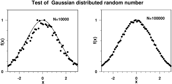
Appendix C
Numerical integration of the Langevin equation
The Langevin equation describing the motion of a free Brownian particle can be solved analytically to get the mean values of the position and momentum as a function of time . As approaches infinity, the Brownian particle is expected to be in equilibrium with the heat bath. The average value of the kinetic energy of the Brownian particle becomes equal to (the temperature T is here in units of energy, i.e. we set the Boltzman constant ). The one dimensional Langevin equation in space with and neglecting the coordinate dependence of the inertia reads as follows:
| (C.1) |
The analytical solution of the above equation is given by[33]
| (C.2) | |||||
| (C.3) |
where and are the respective initial values. Averaging over all possible realizations of the random force, the mean value of the momentum and coordinate are given by
| (C.4) | |||||
| (C.5) |
The mean values of the square of position and momentum are given as follows:
| (C.6) | |||||
| (C.7) | |||||
The above equation is also solved numerically by integrating it
directly by successive iterations(method explained in chapter 3).
The numerical results are compared with the analytical results for
the cases starting with and .
It is seen from Fig. (C.1) that the numerical results almost
coincide with the analytical solution at any steps. We also see
that the Brownian particle approaches the thermal equilibrium
with the heat bath, i.e., irrespective of the initial momenta. The numerical results for are also very well reproduced.
The errors are within which is comparable
with where is the number of trajectories. These
results establish the accuracy and convergence of our algorithm
for solving the Langevin equation which is subsequently used in
fission dynamics.
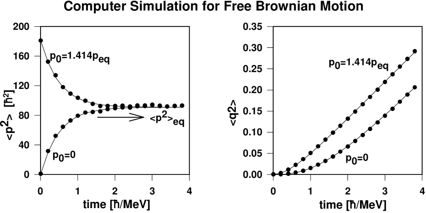
Appendix D
Units and Dimensions
Langevin dynamics
The units and dimensions used for different dynamical variables in the Langevin dynamics will be described here. The different input quantities for the fission dynamics including the shape degrees of freedom for the collective motion are described in details in chapter 2.
(A) Shape degrees of freedom:
and are the shape variables for the fission degrees of
freedom. Both are dimensionless while
( is radius)
has the dimension of length and its unit is . The surface of
the nucleus is
defined by the following expression in cylindrical coordinates,
| (D.1) |
where and are dimensionless (expressions given in section 2.2), has the dimension of length and unit is .
(B) Inertia:
The inertia is given by the following equation, the different
quantities used being already explained in the subsection 2.3.4.
| (D.2) |
In the above expression, is the matter density, the unit is . is the value of on the nuclear surface and hence has the dimension of , unit is . The mathematical definition of is given in section 2.3.4, from which its dimension reduces to that of length, since in our choice of units, ( ) is dimensionless. The unit of being , inertia has the unit of .
(C) Friction:
The friction coefficient is given by the following
expression
| (D.3) |
The unit of (average nucleon speed) is , the units of other quantities being already, defined has the unit of .
(D) Momentum:
It is conventional to express time interval in units of
in the calculations of fission dynamics and we will
also follow the same convention. The following relations will be
useful for the required conversion of units.
| (D.4) |
and
| (D.5) |
It is convenient to express inertia and friction coefficients in units of and MeV. To convert (inverse of inertia) given in units of to that in , one needs to multiply it by the conversion factor as seen is seen from Eq. D.5. Similarly to express the friction coefficient in units of , one needs to divide given in units of by the factor as is evident from Eq. D.4. The equation gives for momentum the units of , being dimensionless. Hence momentum has units of .
(E) Energy:
Energy is expressed in units of MeV and so is the temperature .
It can be checked that the kinetic energy has
units of
MeV.
The units of different input quantities for the Langevin equation
being defined, it can be checked whether the different terms of the
equation has the correct dimensions and units.
The time evolution equation for the momentum is as follows
| (D.6) |
All the quantities in the above Langevin equation is converted and
expressed in units involving and . The l.h.s has unit
of . It can be checked that all the
terms in r.h.s also has the same unit.
( is a number and is hence dimensionless)
Thus it is verified that the system of units used in the Langevin
dynamics is consistent and all the variables has the correct
dimensions.
Particle emission width
In Langevin dynamics, though it is conventional to express time in units of , in the calculation of particle emission widths, time is normally expressed in units of (). Since in our model it is required to couple particle emission with the fission dynamics, appropriate conversions for the corresponding units should be made so that the final dimensions are correct. The particle emission width is given by the following formula
| (D.7) |
The different quantities used in the above equation is explained in section 4.2.4. It is important to note that
| (D.8) |
| (D.9) |
To make proper use of the units, the numerator and denominator of the r.h.s of Eq. D.7 is multiplied by and the final expression has the dimension of (substituting the conversions used in Eqs. D.8 D.9)
| (D.10) |
The decay width thus rightly is expressed in units of and the corresponding decay time which equals is in units of time ()and can be converted to units of using Eq. D.8.
Appendix E
Energetics
The energy conservation followed during the emission of a particle from the compound nucleus is given by the following equation.
| (E.1) |
The subscript is for the parent compound nucleus with mass number , atomic number and neutron number , whereas stands for the daughter nucleus after emission of a particle (subscript ) from the compound nucleus. denotes the mass which for the parent nucleus equals where and are proton and neutron masses respectively. Hence, by definition, will cancel with . stands for the binding energy which is calculated by the liquid drop mass formula of Myers and Swiatecki which is given at the end of this Appendix. If the emitted particle is not a composite particle, i.e, if it is a neutron or a proton then the corresponding binding energy is zero. and gives the excitation energies of the parent and daughter nucleus respectively. is the kinetic energy of the emitted particle which can vary from zero to a maximum value fixed from the above energy balance equation by setting the excitation energy of the daughter nucleus to a minimum possible value. This minimum excitation energy of the daughter nucleus is determined from the considerations of level density of the nucleus which should have some finite value. Zero value of kinetic energy of the emitted particle correspond to maximum excitation of the daughter nucleus. gives the rotational energy of a nucleus with angular momentum and moment of inertia . and gives the angular momenta of the parent and the daughter nucleus where we usually take for the emitted neutron or .
The binding energy of of a nucleus with mass number , proton number and neutron number is given by the liquid drop model of Myers and Swiatecki[134] which is given by the following expression.
| (E.2) |
where
| (E.3) |
and . The first term on the r.h.s of Eq. E.2, i.e., is the sum of the volume energy term which is proportional to the mass number and the volume-asymmetry energy term which is proportional to . The second term is the sum of the surface energy term being proportional to and the surface asymmetry energy term proportional to where equals . The third term is the direct sharp-surface Coulomb energy whereas gives the surface-diffuseness correction to the direct Coulomb energy. The shell correction is not included in the binding energy formula since in fission dynamics of excited nuclei, both the parent and the daughter nuclei are hot, and shell corrections need not be considered. gives the pairing energy correction and is given by the following formulas.
| (E.4) | |||||
Appendix F
Brief description of the computer codes
The different computer codes developed and used in the thesis will be briefly mentioned here. The codes were all written in Fortran language and the computational work was done using ES-40 server with alpha CPU (21264A) having clock speed 667 MHz.
CHAOTICITY
The code named by us as “CHAOTICITY” was obtained from Professor J. Blocki of Institute for Nuclear Research, Swierk, Poland. This code calculates the chaos factor of different nuclear shapes starting from spherical to the scission configuration. The method is based on calculating the Lyapunov exponent of a large number of classical trajectories (typically 10000 or more), from which the chaos factor is extracted. The procedure for calculation of Lyapunov exponent of a trajectory by following it classically in time is explained in section 2.4.3. As part of the thesis work, the above code was modified suitably to incorporate the Brack shape parametrization which is used in our model to represent a hot fissioning nuclei. The initial code as obtained was for volume sampling of trajectories. It was modified by us so that surface sampling of trajectories is possible which is required for our purpose. The chaos factor is calculated for a wide range of the dynamical coordinates and . Values of range from 0.6 to 2.1 in steps of 0.01, whereas for each value of , ranges from -1.5 to 1.5 in steps of 0.1. A typical calculation of chaos factor(for 1000 trajectories) for a particular value of and takes about 2.22 minutes of computer time.
POTFOLD
The code named as “POTFOLD”(POTential FOLDing) was developed as part of this thesis work. This code calculates the potential energy of nuclei of different mass and atomic number as function of the deformation coordinates and . “POTFOLD” includes both the nuclear and the coulomb part of the potential. The potential landscape in coordinates is generated from the finite-range liquid drop model where we calculate the generalized nuclear energy by double folding the uniform density with Yukawa-plus-exponential potential. The Coloumb energy is obtained by double folding another Yukawa function with the density distribution. The detailed description of the potential used can be found in chapter 2 and the techniques used for simplifying and solving the integrals is given in Appendix A. The potential is calculated for the same range of and as the chaos factor mentioned above. A typical calculation of potential for a nuclei of mass number 224 for a particular value of and takes about 8.8 seconds of computer time.
FISSWDTH
The calculation of prescission neutron multiplicity and fission probability proceeds through two stages. In the first part the fission width of a nucleus is calculated dynamically which is required for the next part of the calculation. This code named as “FISSWDTH”(FISSion WiDTH) is developed to calculate the dynamical fission rate or fission width of a nucleus for a particular angular momentum and excitation energy, by numerically solving the Langevin equation. This code considers only one mode of decay of the compound nucleus i.e, fission, and does not include particle or gamma emissions. The fission widths calculated from this code for different values of energy and angular momentum is used for the parametric representation of fission width which serve as input for the statistical branch of the main code(to be described next). The chaos factor and potential which are calculated using the codes mentioned above are used as input for this code. The other inputs required for the calculation of fission width like the friction and inertia are calculated within this code “FISSWDTH”. The different steps involved in the procedure for calculation of fission width is described in section 3.2. A Langevin trajectory is followed in time till it reaches the fission fate and the calculation is repeated for a large number (typically 100,000) of trajectories so that fluctuations in the steady value is minimised (better averaging is possible) and a reliable value of fission width can be extracted from its saturation value. A typical calculation of fission width for thorium nucleus(A=224) for angular momentum and temp MeV takes about 4.72 hours of computer time.
DYSTCNF
This code called “DYSTCNF” is developed as part of the thesis work to calculate the prescission neutron multiplicity and fission probability of different nuclei. The name stands for ‘DYnamical plus STatistical Code for Nuclear Fission’. As the name implies, the code uses a combined dynamical plus statistical model where light particle evaporation is coupled with Langevin dynamics followed by a statistical branch based on Monte Carlo cascade procedure. The different steps of the calculation is discussed thoroughly in section 4.2. The mass and atomic number of target and projectile, laboratory energy of the projectile and value of the reaction are given as inputs to this code. The calculation in the code starts from the formation of a compound nucleus from the fusion of target and projectile, the total excitation energy of the fused nuclei being calculated from the projectile energy and value. The initial conditions for the dynamical coordinates as well as the angular momenta are obtained by sampling suitable distribution functions which are suitably incorporated in different subprograms of the code. The potential values being supplied by the code ’POTFOLD’, a suitable minimization routine finds the minimum in the two dimensional (c,h) valley. Different subprograms are developed in the main code to calculate the free energy, inertia, level density parameter, moment of inertia of the nucleus for different values of the dynamical coordinates and . Wall and Window friction values for different nuclear shapes calculated in a subprogram is suitably combined with the values of the chaos factor obtained from the code ’CHAOTICITY’ to generate the values of the chaos-weighted wall friction values, the testing of which in fission dynamics being the main emphasis of the thesis. The formulas and mathematical expressions for different input parameters calculated in this code are given in chapter 2 of the thesis. The particle emission widths required for the evaporation probability of the particles are calculated within this code while the fission widths are obtained from the separately developed code ’FISSWDTH’. The neutron widths for different mass number(A), angular momentum(l) and excitation energy() of the parent nucleus are calculated and stored by constructing a three dimensional matrix wdthn(i,j,k) where the indices i, j and k stand for mass number, angular momentum and excitation energy respectively. The required values are obtained from this matrix by interpolation. The energy of the emitted particles obtained by sampling the energy spectrum of each type and the binding energy of the emitted particles calculated from the mass of the parent and daughter nuclei using the global liquid-drop parameters of Myers and Swiatecki (Appendix E) are taken care of in different subroutines of the main code. The different time steps like (time step for numerical integration of Langevin equations), (time from where the statistical part of the code starts) and (total time up to which a trajectory is followed) are all given as inputs to this code. The calculation in the code terminates with each trajectory reaching the scission point or ending up as an evaporation residue. A few trajectories may not reach either of these fates within the total specified time (which is chosen to be sufficiently large) and the calculation is stopped there for those trajectories. The whole calculation is repeated for a large ensemble of trajectories and the final outputs like the prescission neutron multiplicity, fission probability or evaporation residue probability are extracted by suitably averaging the numbers obtained from the ensemble. A typical calculation for for 20000 trajectories for projectile energy 100MeV takes about 60 hours of computer time. A schematic sketch of the calculational procedure used in this code is given by the flow chart in Appendix G.
Appendix G
Schematic sketch of the calculational procedure
The flow diagram (Fig. G.1) displays schematically the logical sequence of the actual calculations described in the combined dynamical plus statistical model in chapter 4, which essentially constitutes the code “DYSTCNF” referred in Appendix F . The main steps of the algorithm used in the calculation are shown in the flow chart, others being omitted to make the diagram look simple. The different symbols and logical steps shown in the figure is being explained here. The diagram explains the different steps followed by a trajectory from a compound nucleus till it end up as an evaporation residue or reaches the fission criteria. The flow chart starts with a compound nucleus (CN) of mass with a particular angular momentum and excitation energy . If the excitation energy is less than minimum of (binding energy of neutron) and (fission barrier), then the compound nucleus forms an evaporation residue and adds to which gives the total number of evaporation residue formed. The calculation proceeds if this condition is not satisfied. The dynamical coordinate and momentum at time being given by and respectively, evolve in time following Langevin equations and change over to and , being the time step of integration of the Langevin equations. After each time step, the criteria for scission is checked, i.e, whether the coordinate reaches the scission point . The condition being satisfied, it adds to the total number of fission events which is given by , and the calculation stops there. If the fission condition is not reached, the calculation for the trajectory proceeds to check for the emission of light particles and gamma. The emission of only neutron and gamma is shown in the flow chart. The Monte Carlo selection procedure (described in section 4.2.3) is used to decide whether any emission takes place as well as the type of emission (neutron or ). The energy of the emitted particles is also calculated by Monte-Carlo procedure (not shown in the flow chart), using the integrand of the formula for the corresponding decay width as weight function. The mass number, excitation energy and angular momentum are adjusted properly after each emission of neutron or gamma. gives the energy of the emitted particle. After checking for particle emission, the total elapsed time is compared with . When the total time of calculation in the dynamical branch exceeds the equilibration time and the fission criteria is not yet reached, one switches over to the statistical branch as explained in section 4.2.4. In the statistical branch, the possibility of any particle/ emission or fission and the kind of emission at each time step is checked following the same criteria as in the dynamical branch. The fission width obtained in a separate calculation is used as input for the statistical branch and compared with the particle/ widths to decide the possibilities. The time step in the statistical branch is redefined after each step as , where , and . The final fate of a trajectory (fission or evaporation residue) may be reached from either the dynamical part or the statistical one, each adding up to the respective numbers or . The total number of neutrons emitted in the dynamical branch () is added to that emitted from the statistical branch () to get the total number of neutrons . This number is divided by the total number of fission events to get the prescission neutron multiplicity . If a trajectory neither fissions nor reaches the evaporation residue within the total time specified for the combined dynamical plus statistical calculation, then the calculation is stopped there with the fate of the trajectory still undecided. However, is taken to be sufficiently long so that the number of such “undecided” trajectories is statistically insignificant.
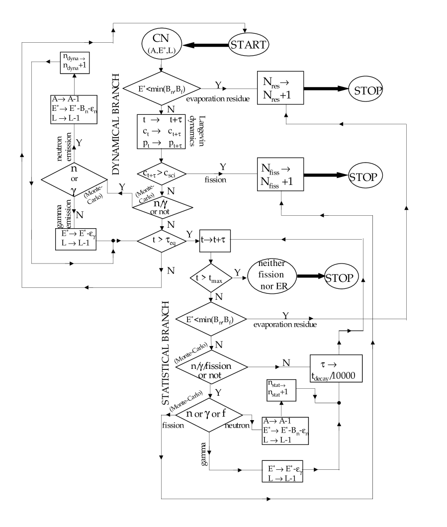
Bibliography
- [1] H.A. Weidenmüller, Progress Particle Nucl. Phys. 3 (1980) 49.
- [2] W. Nörenberg, Nucl. Phys. A 428 (1984) 177c.
- [3] J.R.Birkelund, L.E.Tubbs, J.R. Huizenga, J.N. De and D. Sperber, Phys. Rep. 56 (1979) 107.
- [4] D.H.E. Gross, H. Kalinowski, Phys. Rep. 45 (1978) 175.
- [5] N. Bohr, F. Kalckar, Kgl. Danske Videnskab. Selskab, Mat. Fys. Medd. 14 (1937) (10).
- [6] L. Meitner, O.R. Frisch, Nature 143 (1939) 239.
- [7] N. Bohr, J. A. Wheeler, Phys. Rev. 56 (1939) 426.
- [8] H. A. Kramers, Physica (Amsterdam) 7 (1940) 284.
- [9] A. Bohr, B. R. Mottelson, Kgl. Danske Videnskab. Selskab, Mat. Fys. Medd. 27 (1953) (16).
- [10] P. Ring, P. Schuck, The Nuclear Many Body Problem, Springer, Berlin, 1980.
- [11] G.F. Bertsch, S. Das Gupta, Phys. Rep. 160 (1988) 189.
- [12] H. Hofmann, P.J. Siemens, Nucl. Phys. A 257 (1976) 165.
- [13] H. Hofmann, P.J. Siemens, Nucl. Phys. A 275 (1977) 464.
- [14] W. Nörenberg, H. A. Weidenmüller, Lecture notes in Physics, vol. 51, 2nd ed., Springer, Heidelberg, 1980.
- [15] M.C. Nemes, H.A. Weidenmüller, Phys. Rev. C 24 (1981) 450 and 944.
- [16] W. Cassing and W. Nörenberg, Nucl. Phys. A 401 (1983) 467.
- [17] W. Nörenberg, Nucl. Phys. A 409 (1983) 191c.
- [18] H. Risken, The Fokker-Planck Equation, 2nd ed., Springer, Berlin, 1989.
- [19] N.G. Van Kampen, Stochastic Processes in Physics and Chemistry, North-Holland, Amsterdam, 1981.
- [20] P. Hänggi, P. Talkner and M. Borkovec, Rev. Mod. Phys, 62 (1990) 251.
- [21] W. Nörenberg, Phys. Lett. B 52 (1974) 289.
- [22] P. Hänggi, J. Stat. Phys. 42 (1986) 105.
- [23] A.O. Calderia, A.J. Leggett, Ann. Phys. 149 (1983) 374.
- [24] H. Hofmann, R. Samhammer and G. Ockenfu, Nucl. Phys. A 496 (1989) 269.
- [25] H. Hofmann, G. L. Ingold, Phys. Lett. B 264 (1991) 253.
- [26] H. Hofmann, G. L. Ingold and M. H. Thoma, Phys. Lett. B 317 (1993) 489.
- [27] H. Hofmann, F. Ivanyuk, Phys. Rev. Lett. 82 (1999) 4603
- [28] L.C. Vaz, D. Logan, E. Duck, J.M. Alexander, M.F. Rivet, M.S. Zisman, M. Kaplan, and J.W. Ball, Z. Phys. A 315 (1984) 169; also see, N.N. Ajitanand et. al., Z. Phys. A 316 (1984) 169.
- [29] D.J. Hinde, R.J. Charity, G.S. Foote, J.R. Leigh, J.O. Newton, S. Ogaza and A. Chatterjee, Phys. Rev. Lett. 52 (1984) 986, erratum: 53 (1984) 2275.
- [30] M. Thoennessen, D.R. Chakrabarty, M.G. Hermann, R. Butsch, and P. Paul, Phys. Rev. Lett. 59 (1987) 2860
- [31] S. Hassani and P. Grangé, Phys. Lett. B 137 (1984) 281.
- [32] P. Grangé, Li Jun-Qing and H.A. Weidenmüller, Phys. Rev. C 27 (1983) 2063.
- [33] Y. Abe, C. Gregoire, H. Delagrange, J. Phys. C4 (47) (1986) 329.
- [34] V.M. Strutinsky, Phys. Lett. B 47 (1973) 121.
- [35] P. Grangé and H.A. Weidenmüller, Phys. Lett. B 96 (1980) 26.
- [36] A. Gavron et. al., Phys. Rev. Lett. 47 (1981) 1255, erratum: 48 (1982) 835. A. Gavron et. al., Phys. Lett. B 176 (1986) 312.
- [37] P. Grangé, Nucl. Phys. A 428 (1984) 37.
- [38] Wu. Xi-Zhen and Zhuo Yi-Zhong, Chin. Phys. 1 (1981) 671.
- [39] H. Delagrange et al. Z. Phys. A 323 (1986) 437.
- [40] D.J. Hinde, D. Hilscher and H. Rossner, Nucl. Phys. A 502 (1989) 497c.
- [41] C. Gregoire, H. Delagrange, K. Pomorski, K. Dietrich, Z. Phys. A 329 (1988) 497.
- [42] E. Strumberger, K. Dietrich and K. Pomorski, Nucl. Phys. A 529 (1991) 522.
- [43] G.D. Adeev, I.I. Gontchar, V.V. Pashkevich, N.I. Pischasov, and O.I. Serdyuk, Sov. J. Part. Nucl. 19 (1988) 529.
- [44] J. Randrup, Nucl. Phys. A 327 (1979) 490.
- [45] K.E. Rehm, Phys. Lett. B 86 (1979) 260.
- [46] V.C. Barbosa, P.C. Soares, E.C. Oliveira, L.C. Gomes, Rev. Bras. Fiz. 15 (1985) 211.
- [47] P. Fröbrich, in: H. Feldmeier(Ed.), Proc. Gross properties of nuclei and nuclear excitations XV, Hirschegg, Austria, (1987) 230.
- [48] Y. Abe, S. Ayik, P.-G. Reinhard, E. Suraud, Phys. Rep. 275 (1996) 49.
- [49] U. Eckern et al., J. Stat. Phys. 59 (1990) 885.
- [50] H. Hofmann, R. Samhammer and S. Yamaji, Phys. Lett. B 229 (1989) 309.
- [51] V. Weisskopf, Phys. Rev. 52 (1937) 295.
- [52] F. Pühlhofer, Nucl. Phys. A 280 (1977) 267.
- [53] M. Blann, Beckerman, Nucleonika 23 (1978) 34.
- [54] D. Hilscher, E. Holub, U. Jakuke, H. Orf, H. Rossner, Proc. 3rd adriatic Europhysics Conf. on dynamics of Heavy-ion collisions, Hvar, Yugoslavia, North-Holland, Amsterdam, (1981) 225.
- [55] S. Hassani, P. Grangé, Z. Phys. A 325 (1986) 95.
- [56] H. A. Weidenmüller, Nucl. Phys. A 471 (1987) 1c.
- [57] W.P. Zank, D. Hilscher, G. Ingold, U. Jahnke, M. Lehmann, H. Rossner, Phys. Rev. C 33 (1986) 519.
- [58] A. Gavron. et al., Phys. Rev. C 35 (1987) 579.
-
[59]
P. Grangé, P. Hassani, H.A. Weidenmüller, A.
Gavron, J.R. Nix, A.J. Sierk,
Phys. Rev. C 34 (1986) 209. - [60] D.J. Hinde, R.J. Charity, G.S. Foote, R.J. Leigh, J.D. Newton, S. Osaza, A. Chatterjee, Nucl. Phys. A 452 (1986) 550.
- [61] J.P. Lestone et. al., Phys. Rev. Lett. 67 (1991) 1078.
- [62] J.O.Newton, D.J.Hinde, R.J. Charity, J.J.M. Bokhorst, A. Chatterjee, G.S. Foote, S. Ogaza, Nucl Phys. A 483 (1988) 126.
- [63] M. Thoennessen, G.F. Bertsch, Phys. Rev. Lett.. 71 (1993) 4303.
- [64] J.O. Newton, Sov. J. Part. Nucl. 21 (1990) 349.
- [65] D. Hilscher, H. Rossner, Ann. Phys. Fr. 17 (1992) 471.
- [66] D.J. Hinde, Nucl. Phys. A 553 (1993) 255c.
- [67] P. Paul, M. Thoennessen, Ann. Rev. Part. Nucl. Sci. 44 (1994) 65.
- [68] D. Hilscher, I.I. Gontchar and H. Rossner, Physics of Atomic Nuclei 57 (1994) 1187.
- [69] D.J. Hofman, B.B. Back and P. Paul, Phys. Rev. C 51 (1995) 2597.
- [70] W. Nörenberg, Z. Phys. A 274 (1975) 241.
- [71] W. Nörenberg, Z. Phys. A 276 (1976) 84.
- [72] D.H.E. Gross, Nucl Phys. A 240 (1975) 472.
- [73] J. Blocki, Y. Boneh, J.R. Nix, J. Randrup, M. Robel, A.J. Sierk, and W.J. Swiatecki, Ann. Phys. 113 (1978) 330.
- [74] K.T.R. Davies, A.J. Sierk, J.R. Nix, Phys. Rev. C 13 (1976) 2385.
- [75] K.T.R. Davies, R.A. Managan, J.R. Nix, A.J. Sierk, Phys. Rev. C 16 (1977) 1890.
- [76] P. Grange, H.C. Pauli, H.A. Weidenmüller, Phys. Lett. B 88 (1979) 9.
- [77] P. Grange, H.C. Pauli, H.A. Weidenmüller, Z. Phys. A 296 (1980) 107.
- [78] G.D. Adeev, I.I. Gontchar, Yad. Fiz. 37 (1983) 1113.
- [79] G.D. Adeev, I.I. Gontchar, Yad. Fiz. 40 (1984) 869.
- [80] G.D. Adeev, I.I. Gontchar, Z. Phys. A 320 (1985) 451.
- [81] G.D. Adeev, I.I. Gontchar, L.A. Marchenko, N.I. Pishasov, Yad. Fiz. (1986) 1137.
- [82] G.D. Adeev, I.I. Gontchar, Z. Phys. A 322 (1985) 479.
- [83] O.I. Serdyuk, G.D. Adeev, I.I. Gontchar, V.V. Pashkevich, N.I. Pishasov, Yad. Fiz. 46 (1987) 710, translated in Sov. J. Nucl. Phys. 46, 399.
- [84] G.D. Adeev, I.I. Gontchar, L.A. Marchenko, Yad. Fiz.42 (1985) 42.
- [85] P. Fröbrich, I.I. Gontchar, Phys. Rep. 292 (1998) 131.
- [86] P. Fröbrich, I.I. Gontchar, Nucl. Phys. A 563 (1993) 326.
- [87] K. -T, Brinkmann, A.L. Caraley, B.J. Fineman, N. Gan, J. Velkovska, and R.L. McGrath, Phys. Rev. C 50 (1994) 309.
- [88] Yu.A. Lazarev, I.I. Gontchar and N.D. Maviltov, Phys. Rev. Lett. 70 (1993) 1220.
- [89] D.J. Hofman et al., Phys. Rev. Lett. 72 (1994) 470.
- [90] H. Hofmann, Phys. Rep. 284 (4 & 5) (1997) 137.
- [91] S. Yamaji, F.A. Ivanyuk, H. Hofmann, Nucl. Phys. A 612 (1997) 1.
- [92] H. Hofmann, F.A. Ivanyuk, and S. Yamaji, Nucl. Phys. A 598 (1996) 187.
- [93] H. Hofmann, F. A. Ivanyuk, A. G. Magner, Acta Phys. Polon. B 29 (1998) 375.
- [94] F.A. Ivanyuk, Z. Phys. A 334 (1989) 69.
- [95] A.G. Magner, H. Hofmann, V.M. Kolomietz and S. Shlomo, Phys. Rev. C 51 (1995) 2457.
- [96] B.W. Bush, G.F. Bertsch and B.A. Brown, Phys. Rev C 45 (1992) 1709.
- [97] D. Cha and G.F. Bertsch, Phys. Rev. C 46 (1992) 306.
- [98] D. Boiley, E. Suraud, Y. Abe, ans S. Ayik, Nucl. Phys. A 556 (1993) 67.
- [99] F.A. Ivanyuk, K. Pomorski, Phys. Rev. C 53 (1996) 1861.
- [100] H. Hofmann, F.A. Ivanyuk, C. Rummel and S. Yamaji, Phys. Rev. C 64 054316 (2001).
- [101] T. Wada, Y. Abe, N. Carjan, Phys. Rev. Lett. 70 (1993) 3538.
- [102] S.E. Koonin, R.L. Hatch, J. Randrup, Nucl. Phys. A 283 (1977) 87.
- [103] S. Yamaji, H. Hofmann and R. Samhammer, Nucl. Phys. A 475 (1988) 487.
- [104] J. Blocki, J. Skalski, W.J. Swiatecki, Nucl. Phys. A 594 (1995) 137.
- [105] J. Blocki, M. Dworzecka, F. Beck, and H. Feldmeier, Phys. Lett. B 99 (1981) 13.
- [106] A.J. Sierk and J.R. Nix, Phys. Rev. C 21 (1980) 982.
- [107] J.R. Nix and A.J. Sierk, Phys. Rev. C 21 (1980) 396; C 25 (1982) 1068.
- [108] W.D. Myers, W.J. Swiatecki, T. Kodama, L.J. El-Jaick, and E.R. Hilf. Phys. Rev. C 15 (1977) 2032.
- [109] J.R. Nix and A.J. Sierk, in Proceedings of the International School- Seminar on Heavy Ion physics, Dubna, USSR, (1986), Report No. JINR-D7-87-68, 1987, p. 453; J. R. Nix, Nucl. Phys. A 502 (1989) 609c.
- [110] J.R. Nix and A.J. Sierk, in Proceedings of the 6th Adriatic Conference on Nuclear Physics: Frontiers of Heavy Ion Physics, Dubrovnik, Yugoslavia,1990, edited by N. Cindro, R. Caplar and W. Greiner (World Scientific, Singapore, 1990), p. 333.
- [111] J.Blocki, J.-J.Shi and W.J.Swiatecki, Nucl. Phys. A 554 (1993) 387.
- [112] J. Blocki, F. Brut and W.J. Swiatecki, Nucl. Phys. A 554 (1993) 107.
- [113] J. Blocki, C. Jarzynski and W.J. Swiatecki, Nucl. Phys. A 599 (1996) 486.
- [114] J. Blocki, F. Brut and W.J. Swiatecki, Acta Phys. Pol. B 25 (1994) 637.
- [115] J. Blocki, J. Skalski and W.J. Swiatecki, Nucl. Phys. A 618 (1997) 1.
- [116] P. Magierski, J. Skalski and J. Blocki, Phys. Rev. C 56 (1997) 1011.
- [117] J. Blocki, F. Brut, T. Srokowski and W.J. Swiatecki, Nucl. Phys. A 545 (1992) 511c.
- [118] Oriol Bohigas, H. A. Weidenmüller, Ann. Rev. Nucl. Part. Sci. 38 (1988) 422.
- [119] W. J. Swiatecki, Nucl. Phys. A 488 (1988) 375c.
- [120] C. Yannonleas, Nucl. Phys. A 439 (1985) 336.
- [121] J.J. Griffin and M. Dowrzecka, Nucl Phys. A 455 (1986) 61.
- [122] S.E. Koonin and J. Randrup, Nucl. Phys. A 289 (1977) 475.
- [123] Santanu Pal and Tapan Mukhopadhyay, Phys. Rev. C 54 (1996) 1333.
- [124] Y. Abe, B. Bouriquet, Acta Phys. Polon. 34 (2003) 1927.
-
[125]
V. S. Stavinsky, N. S. Rabotnov, and A. A.
Seregin, Yad. Fiz. 7 (1968) 1051;
V. V. Pashkevich, Nucl. Phys. A 169 (1971) 275. - [126] G.D. Adeev and P.A. Cherdantsev, Phys. Lett. B 39 (1972) 485; G.D. Adeev and P.A. Cherdantsev, Yad. Fiz. 18 (1973) 741.
- [127] G.R. Tillack, Phys. Lett. B 278 (1992) 403.
- [128] N. Carjan, A.J. Sierk and J.R. Nix, Nucl. Phys. A 452 (1986) 381, and refernces therein.
- [129] M. Brack, J. Damgard, A.S. Jensen, H.C. Pauli, V.M. Strutinsky, C.Y. Wong, Rev. Mod. Phys. 44 (1972) 320.
- [130] R. W. Hasse and W. D. Myers, Geometrical Relationships of Macroscopic Nuclear Physics (Springer-Verlag, Berlin, 1988)
- [131] M. Brack, C. Guet, H.-B. Hakansson, Phys. Rep. 123 (1985) 275.
- [132] J. Bartel, M. Brack, M. Durand, Nucl. Phys. A 445 (1985) 263.
- [133] A.J. Sierk, Phys. Rev. C 33 (1986) 2039.
- [134] W.D. Myers, W.J. Swiatecki, Ark. Phys. 36 (1967) 343; Nucl. Phys. 81(1966) 1.
- [135] S. Cohen, F. Plasil, and W. J. Swiatecki, Ann. Phys. (N.Y.) 82 (1974) 557.
- [136] H. J. Krappe, J. R. Nix, and A. J. Sierk, Phys. Rev. Lett. 42 (1979) 215; Phys. Rev. C 20 (1979) 992.
- [137] K.T.R. Davies and J.R. Nix, Phys. Rev. C 14 (1976) 1977.
- [138] P. Möller and J. R. Nix, Nucl. Phys. A 361 (1981) 117; At. Data Nucl. Data Tables 26 (1981) 165.
- [139] D. V. Vanin, G. I.. Kosenko, and G.D. Adeev, Phys. Rev. C 59 (1999) 2114; Phys. At. Nucl. 63 (2000) 1865.
- [140] A.V. Ignatyuk, M.G. Itkis, V.N. Okolovich, G.N. Smirenkin, and A.S. Tishin, Yad. Fiz. 21 (1975) 1185. [Sov. J. Nucl. Phys. 21 (1975) 612.]
- [141] R. Balian and C. Bloch, Ann. Phys. (N.Y.) 60 (1970) 401.
- [142] J. Toke, W.J. Swiatecki, Nucl. Phys. A 372 (1981) 141.
- [143] I.I. Gontchar, P. Fröbrich, and N.I. Pischasov, Phys. Rev C 47 (1993) 2228; I.I. Gontchar, P. Fröbrich, Nucl. Phys. A 551 (1993) 495.
- [144] A.V. Karpov, P.N. Nadtochy, E.G. Ryabov and G.D. Adeev, J. Phys. G: Nucl. Part. Phys. 29 (2003) 2365.
- [145] H.J. Krappe, Phys. Rev. C 59 (1999) 2640.
- [146] C. Guet, E. Strumberger, and M. Brack, Phys. Lett. B 205 (1988) 427.
- [147] A. Bohr and B.R. Mottelson, Nuclear structure, Vol. II, Benjamin, London, 1975.
- [148] H. Hofmann, Phys. lett. B 61 (1976) 423.
- [149] J. R. Nix, Nucl. Phys. A 130 (1969) 241.
- [150] P. Fröbrich, I.I. Gontchar, N.D. Maviltov, Nucl. Phys. A 556 (1993) 281.
- [151] A. V. Karpov, P.N. Nadtochy, D.V. Vanin, and G.D. Adeev, Phys. Rev. C 63 (2001) 054610.
- [152] P.N. Nadtochy, G.D. Adeev, and A.V. Karpov, Phys. Rev. C 65 (2002) 064615.
- [153] Martin C. Gutzwiller, Chaos in Classical and Quantum Mechanics (Springer, Berlin, 1990)
- [154] R. Arvieu, F. Brut, J. Carbonell, and J. Touchard, Phys. Rev. A 35 (1987) 2389.
- [155] I.C. Percival, J. Phys. B 6 (1973) L229.
- [156] T. Mukhopadhyay and S. Pal, Phys. Rev. C 56 (1997) 296.
- [157] S. Pal and T. Mukhopadhyay, Phys. Rev. C 57 (1998) 210.
- [158] Gargi Chaudhuri and S. Pal, Phys. Rev. C 65 (2002) 054612.
- [159] I. Diószegi, N.P. Shaw, I. Mazumdar, A. Hazikoutelis, and P. Paul, Phys. Rev. C 61 (2000) 024613-1.
- [160] N.P. Shaw et al., Phys. Rev. C 61 (2000) 044612-1.
- [161] I. Diószegi et al., Phys. Rev. C 63 (2000) 014611-1.
- [162] T. Wada, N. Carjan, and Y. Abe, Nucl. Phys. A 538 (1992) 283c.
- [163] P. Langevin, Comptes Rendus de l’ Academic des Sciences 146 (1908) 530.
- [164] G.E. Uhlenbeck and L.S. Ornstein, Phys. Rev. 36 (1930) 823.
- [165] S. Chandrasekhar, Rev. Mod. Phys. 15 (1943) 1.
- [166] Y. Abe, D. Boiley, B.G. Giraud,T. Wada, Phys. Rev. E 61 (2000) 1125.
- [167] O. Mazonka, C. Jarzynski and J. Blocki, Nucl. Phys. A 641 (1998) 335.
- [168] V. M. Strutinsky, N. Ya. Lyashchenko, and N.A. Popov, Nucl. Phys. 46 (1962) 639.
- [169] U. Brosa, S. Grossmann, and A. Müller, Phys. Rep. 197 (1990) 167.
- [170] G. D. Adeev and V. V. Pashkevich, Nucl. Phys. A 502 (1989) 405c.
- [171] G.I. Kosenko, I.I. Gontchar, N. I. Pischasov, and O.I. Serdyuk, Sov. J. Nucl. Phys. 55 (1992) 514.
- [172] J. Bao, Y. Zhuo, and X. Wu, Z. Phys. A 352 (1995) 321.
- [173] G. D. Adeev and P. N. Nadtochy, Phys. At. Nucl. 66 (2003) 618.
- [174] Gargi Chaudhuri and S. Pal, Phys. Rev. C63 (2001) 064603.
- [175] J.S. Forster, L.V. Mitchell, J.U. Anderson, A.S. Jensen, E. Laegsgard, W.M. Gibson, and K. Reichelt, Nucl Phys. A 464 (1987) 497.
- [176] D. Fabris, G. Viesti, E. Fioretto, M. Cinausero, N. Gelli, K. Hagel, F. Lucarelli, J.B. Natowitz, G. Nebbia, G. Prete, and R. Wada, Phys. Rev. Lett. 73 (1994) 2676.
- [177] K. Pomorski, B. Nerlo-Pomorska, A. Surowiec, M. Kowal, J. Bartel, K. Dietrich, J. Richert, C. Schmitt, B. Benoit, E. de Goes Brennand, L. Donadille, and C. Badimon, Nucl. Phys. A 679 (2000) 25.
- [178] N.D. Maviltov, P. Fröbrich, and I.I. Gontchar, Z. Phys. A 342 (1992) 195.
- [179] P. N. Nadtochy, A.V. Karpov, D.V. Vanin, and G.D. Adeev, Phys. At. Nucl. 66 (2003) 1203.
- [180] J. Marten, P. Fröbrich, Nucl. Phys. A 545 (1992) 854.
- [181] Nuclear Wallet Cards, Isotope Project, NNDC, Lawerence Berkeley Laboratory.
- [182] W. D. Myers, Droplet Model of Atomic Nuclei, IFI/ Plenum Data Company, New York (1977).
- [183] P. Fröbrich, Nucl. Phys. A 545 (1992) 87c.
- [184] Y. Abe, N. Carjan, M. Ohta and T. Wada, Proc. IN2P3-RIKEN Symp. on Heavy-Ion Collisions, Obernai, (1990) France.
- [185] K. Pomorski, J. Bartel, J. Richert, K. Dietrich, Nucl. Phys. A 605 (1996) 87.
-
[186]
J.E. Lynn, Thoery of Neutron Resonance Reactions,
Clarendon, Oxford, 1968,
p. 325. - [187] D.J. Hinde, D. Hilscher, H. Rossner, B. Gebaure, M. Lehmann, and M. Wilpert, Phys. Rev. C 45 (1992) 1229.
- [188] D.J. Hinde, H. Ogata, M. Tanaba, T. Shimoda, N. Takahashi, A. Shinohara, S. Wakamatsu, K. Katori, and H. Okamura, Phys. Rev. C 39 (1989) 2268.
- [189] H. Rossner, D.J. Hinde, J.R. Leigh, J.P. Lestone, J.O. Newton, J.X. Wei, and S. Elfstrom, Phys. Rev. C 45 (1992) 719.
- [190] R.J. Charity, J.R. Leigh, J.J.M. Bokhorst, A. Chatterjee, G.S. Foote, D.J. Hinde, J.O. Newton, S. Ogaza, and D. Ward, Nucl. Phys. A 457,(1986) 441.
- [191] J. Lestone et al., Phys. Rev. Lett. 70 (1993) 2245.
- [192] B.B. Back, D.J. Blumenthal, C.N. Davids, D.J. Henderson, R. Hermann, D.J. Hofman, C.L. Jiang, H.T. Pentilä, and A.H. Wuosmaa, Phys. Rev. C 60 (1999) 044602-1.
- [193] C.R. Morton, D.J. Hinde, J.R. Leigh, J.P. Lestone, M. Dasgupta, J.C. Mein, J.O. Newton, and H. Timmers, Phys. Rev. C 52 (1995) 243.
- [194] Gargi Chaudhuri and Santanu Pal, Eur. Phys. J. A 18 (2003) 9.
- [195] F.P. Heberger, V. Ninov and U. Spoerel, Z. Phys. A 340 (1991) 171.
- [196] K. H. Bhatt, P. Grange and B. Hiller, Phys. Rev. C 33 (1986) 954.
- [197] Hans A. Weidenmüller and Zhang Jing-Shang, Phys. Rev. C 29 (1984) 879.
- [198] R. Butsch, D. J. Hofman, C. P. Montoya, P. Paul and M. Thoennessen, Phys. Rev. C 44 (1991) 1515.
- [199] B. Jurado, K.-H. Schmidt, J. Benlliure, Phys. Lett. B 553 (2003) 186.
- [200] B. Jurado, C. Schmitt, K.-H. Schmidt, J. Benlliure, A.R. Junghans, arXiv: nucl-ex/0302003, submitted to Nucl. Phys. A.
- [201] B. Jurado, C. Schmitt, K.-H. Schmidt, J. Benlliure, A.R. Junghans, arXiv: nucl-ex/0403004.
- [202] S.K.Hui, C.R. Bhuniya, A.k. Ganguly, N.Madhavan, J.J.Das, P.Sugathan, D.O. Kataria, S. Murlithar, L.T. Baby, V. Tripathi, A. Jhingan, A.K. Sinha, P.V. Madhusudhana Rao, N.V.S.V. Prasad, A. M. Vinodkumar, R. Singh, M. Thoennessen, G. Gervais, Phys. Rev C 62 (2000) 054604, Comment: Phys. Rev. C 64 (2001) 019801, Reply: Phys. Rev. C 64 (2001) 019802.
- [203] B. Jurado, C. Schmitt, K.-H. Schmidt, J. Benlliure, T. Enqvist, A.R. Junghans, J. Benlliure, A. Kelić, F. Rejmund, arXiv: nucl-ex/0401013.
- [204] J. Benlliure, P. Armbruster, M. Bernas, A. Boudard, T. Enqvist, R. Legrain, S. Leray, F. Rejmund, K.-H. Schmidt, C. Stéphan, L. Tassan-Got, C. Volant, Nucl. Phys. A 700 (2002) 469.
- [205] Gargi Chaudhuri and Santanu Pal, Eur. Phys. J. A 14 (2002) 287.
- [206] P. Fröbrich, G. R. Tillack, Nucl, Phys. A 540 (1992) 353.
- [207] C. Schmitt, J. Bartel, K. Pomorski, A. Surowiec, Acta Phys. Polon. B 34 (2003) 1651.
- [208] V.M. Kolomietz, S.V. Radionov, S. Shlomo, Phys. Rev. C 64 (2001) 054302.
- [209] H. Hofmann, F.A. Ivanyuk, Phys. Rev. Lett. 90 (2003) 132701.
- [210] H. Hofmann, Phys. Lett. B 567 (2003) 189.
- [211] K.-H. Schmidt, J. Benlliure, D. Boilley, A. Heinz, A. Junghans, B. Jurado, A. Kelic, J. Pereira, C. Schmitt, O. Yordanov, arXiv: nucl-th/0307097.
- [212] H. Hofmann, F.A. Ivanyuk, Heavy Ion Phys. 18 (2003) 377 (arXiv: nucl-th/0210004).
- [213] H. Hofmann, A.G. Magner, Phys. Rev. C 68 (2003) 014606.
- [214] Jing-Dong Bao and Ying Jia, Phys. Rev. C 69 (2004) 027602.
- [215] R. J. Charity, arXiv:nucl-th/0406040.
- [216] A.C. Berriman et al., Nature(London) 413 (2001), 144.
- [217] D.J. Hinde, M. Dasgupta, and A. Mukherjee, Phys. Rev. Lett. 89 (2002) 282701-1.
- [218] W.U. Schröder, J.R. Huizenga, “Treatise on Heavy-Ion Science”, ed. D.A. Bromley, Vol. 2, Plenum Press New York and London (1984) 115.
- [219] B. Lott, F. Goldenbaum, A. Böhm, W. Bohne, T. von Egidy, P. Figuera, J. Galin, D. Hilscher, U. Jahnke, J. Jastrzebski, M. Morjean, G. Pausch, A. Péghaire, L. Pienkowski, D. Polster, S. Proschitzki, B. Quednau, H. Rossner, S. Schmid, W. Schmid, Phys. Rev. C 63 (2001) 034616.
- [220] P. Hofmann, A. S. Iljinov, Y. S. Kim, M. V. Mebel, H. Daniel, P. David, T. von Egidy, T. Haninger, F. J. Hartmann, J. Jastrezbeski, W. Kurzewicz, J. Lieb, H. Machner, H. S. Plendl, G. Riepe, B. Wright, K. Ziock, Phys. Rev. C 49 (1994) 2555.
- [221] Y. S. Kim, A. S. Iljinov, M. V. Mebel, P. Hofmann, H. Daniel, T. von Egidy, T. Haninger, F. J. Hartmann, H. Machner, H. W. Plendl, G. Riepe, Phys. Rev. C 54 (1996) 2469.
- [222] W. Schmid, T. von Egidy, F. J. Hartmann, J. Hoffmann, S. Schmid, D. Hilscher, D. Polster, H. Rossner, A. S. Iljinov, M. V. Mebel, D. I. Ivanov, V. G. Nedorezov, A.S. Sudov. H. Machner, H. S. Plendl, J. Eades, S. Neumaier, Phys. Rev. C 55 (1997) 2965.
- [223] E-M. Eckert, A. K hmichel, J. Pochodzalla, K. D. Hildenbrand, U. Lynen, W. F. J. M ller, H. J. Rabe, H. Sann, H. Stelzer, W. Trautmann, R. Trockel, R. Wada, A. Cerruti, P. Lh noret, R. Lucas, C. Mazur, C. Ng , M. Ribrag, E. Tomasi, A. Demeyer, D. Guinet, Phys. Rev. Lett. 64 (1990) 2483.
- [224] B. Jurado, C. Schmitt, K.-H. Schmidt, J. Benlliure, T. Enqvist, A.R. Junghans, J. Benlliure, A. Kelić, F. Rejmund, arXiv: nucl-ex/0403006.
- [225] P. Fröbrich, arXiv: nucl-th/0401045. (to be published in Progress of Theoretical Physics).