QCD sum rules for nucleon two-point function in nuclear medium

Abstract

We derive QCD sum rules from the nucleon two-point function in nuclear medium, calculating its specral function in chiral perturbation theory to one loop. Our calculation shows the inadequacy of the commonly used ansatz to represent the two-point function as the sum of a nucleon pole term and a spectral integral over the high energy continuum. We also point out that it is the energy variable and not its square that must be used in writing the dispersion integrals. The sum rules are obtained by equating terms linear in nucleon number density of the spectral and operator representations of the correlation function. We use them to predict the curent-nucleon coupling, in good agreement with the value known from the vacuum sum rules. They also predict a definite deviation of the four-quark condensate from its ground state saturation value.

PACS numbers: 12.38.Lg, 12.39.Fe, 24.85.+p

I introduction

The extension of the original QCD sum rules [1] to finite temperature and chemical potential has been the subject of many investigations [2, 3]. These were first extended to finite temperature by Bochkarev and Shaposhnikov [4], who pointed out the importance of continuum contribution in the low energy region. Working with the two-point function of vector currents, they showed that the contribution of the $\pi\pi$ intermediate state, though negligible in vacuum compared to that of the $\rho$-pole, is important at finite temperature.

As shown by Leutwyler and Smilga [5], chiral perturbation theory provides a reliable method to calculate the correlation functions. They took the two-point function of nucleon currents at finite temperature and considered all the one-loop Feynman graphs of this theory to calculate the nucleon pole parameters at finite temperature. Later Koike [6] worked out directly the absorptive parts of these graphs to construct their spectral representations. He then evaluated the QCD sum rules in agreement with known results.

The sum rules at finite temperature were subsequently taken up in Refs. [7, 8], where their spectral sides were calculated from the set of all one-loop Feynman graphs with vertices from chiral perturbation theory. It was shown that the contribution of each graph can, in general, be separated into a pole term for the communicating single particle and a remainder, that is finite at the pole. Clearly to evaluate the changes in the pole paramters, the remainder terms are not necessary. But in the evaluation of the sum rules, where we require their contributions at large external momenta, both the pole term and the remainder are of comparable magnitude.

This observation questions the widely used ansatz for the two-point function given by a pole term (with modified parameters) together with continuum contributions from high energy region only. Such an Ansatz ignores the equally important contribution from the contiuuum in the low energy region and is therefore incomplete.

In this work we investigate the QCD sum rules derived from the two-point function of nucleon currents at finite nucleon chemical potential [9, 10]. Our work concerns the spectral side of the sum rules. As at finite temperature, we work out the spectral representation in nuclear medium in chiral perturbation theory to one loop. The contribution of the Feynman graphs are separared into the nucleon pole term and a continuum contribution in the low energy region. Again we find the Borel transform of these two types of terms to be of comparable magnitude.

Another point overlooked in the literature is the absence of any symmetry of the amplitudes in the energy variable in the present case. Unlike in pionic medium (at finite temperature), the two-point function in nuclear medium has no density dependent singularities from the ‘crossed channel’, as we have no antinucleons in the medium. Thus if $q$ is the external four-momentum and we restrict to $q_{\mu}=(q_{0}=E,\vec{q}=0)$, there is no absorptive part of the amplitudes for $E<0$. Clearly the amplitudes have no symmetry under $E\rightarrow-E$. As a result the dispersion variable must be $E$ and not $E^{2}$.

We also address the issue of sensitivity of the sum rules. The in-medium sum rules, as they are generally written, are actually the corresponding vacuum sum rules, to which are added density dependent contributions. If the vacuun sum rule is stable in a region of the Borel parameter and the density dependent ‘corrections’ are small, as is usually the case, it is likely that the stability of the in-medium sum rules do not depend sensitively on these corrections.

To restore the sensitivity of our sum rules, we equate terms linear in the nucleon number density on the spectral and the operator sides of the two-point function. Our in-medium sum rules are thus independent of the vacuum sum rule, being built out of the ‘correction terms’ only. We recall here that in the vacuum sum rules the unit operator provides the dominant contribution on the operator side, to which higher dimension operators add small ‘power corrections’. In the present sum rules, the contribution of the unit operator, being independent of density, is absent altogether.

In Sec.II we discuss the ingredients needed to write our sum rules. Here we present the form of the spectral representation given by the real-time field theory in medium. Then we derive the interaction vertices from chiral perturbation theory. We also list here the operators and their Wilson coefficients, that we shall include in expanding the operator product in the two-point function. The spectral representations of different Feynman graphs are worked out in Sec.III. The sum rules are written and evaluated in Sec.IV. In Sec.V we comment on different aspects of our sum rules.

II preliminaries

A Two point function

Although we restrict the sum rules to symmetric nuclear matter at zero temperature, our procedure to derive these is completely general. Thus we start with the ensemble average of the time ordered product of two nucleon ‘currents’,

$$\Pi(q)=i\int d^{4}xe^{iqx}\langle T\eta(x)\bar{\eta}(0)\rangle,$$ (2.1)

where for any operator $O$, $\langle O\rangle=Tr\left[\rho O\right]/Tr\rho~{},\rho=e^{-\beta(H-\mu N)}$, $H$ being the Hamiltonian of the system, $\beta$ the inverse of temperature and $N$ the nucleon number operator with chemical potential $\mu$. The nucleon current $\eta(x)_{D,i}$, with spin and isospin indices $D,\,i$ respectively, is built out of three quark fields, so as to have the quantum numbers of the nucleon [11]. In obtaining the spectral representation, we need only its hadronic matrix elements, but to expand the operator product in (2.1) into local operators, we must know its specific structure. Of the different possibilities, we take here the preferred one [12], which for proton ($i=1$) is

$$\eta_{D,1}(x)=\epsilon^{abc}\left(u^{aT}(x)C\gamma^{\mu}u^{b}(x)\right)\left(\gamma_{5}\gamma_{\mu}d^{c}(x)\right)_{D}\,,$$ (2.2)

where $C$ is the charge conjugation matrix and $a,\,b,\,c$ are the color indices.

It is well-known that in a medium amplitudes take a Lorentz covariant form, if we introduce the four-vector $u^{\mu}$, the four-velocity of the medium. Thus our two point function admits a Dirac decomposition, $\Pi(q)=A(q){\bf 1}+B(q)q\!\!\!/+C(q)u\!\!\!/$. In what follows we write the sum rules for $\vec{q}=0$, when it reduces to $\Pi(q_{0}=E,\vec{q}=0)=A(E){\bf 1}+D(E)\gamma_{0}$.

We shall use the real time version of the field theory in a medium, where a two point function assumes the form of a 2$\times$2 matrix. But the dynamics is given essentially by a single analytic function, that is determined by the $11$-component itself. Thus if $F_{11}(q)$ is the $11$-component of the matrix amplitude, the corresponding analytic function $F(q)$ has the spectral representation [13]

$$F(E,\vec{q})=\frac{1}{\pi}\int\frac{\coth(\beta(E-\mu)/2)ImF_{11}(E^{\prime},\vec{q})}{E^{\prime}-E-iE^{\prime}\epsilon}dE^{\prime}.$$ (2.3)

As the chemical potential for particles and antiparticles are equal and opposite, its presence in Eq.(2.1) leads to a loss of symmetry of the amplitude under $E\rightarrow-E$. The simplest example to observe this asymmetry is provided by the components of the $2\times 2$ matrix of the free nucleon propagator. Denoting the nucleon field by $\psi(x)$, we have for the $11$-component [14],

$$\frac{1}{i}S(p)_{11}\equiv\int d^{4}xe^{ipx}\langle T\psi(x)\bar{\psi}(0)\rangle_{11}=(p\!\!\!/+m)\left[\frac{i}{p^{2}-m^{2}+i\epsilon}-\left\{n^{-}(\omega_{p})\theta(p_{0})+n^{+}(\omega_{p})\theta(-p_{0})\right\}2\pi\delta(p^{2}-m^{2})\right],$$ (2.4)

where $n^{\mp}$ are the distribution functions for nucleons and antinucleons, $n^{\mp}(\omega_{p})=\left\{e^{\beta(\omega_{p}\mp\mu)}+1\right\}^{-1},\,\omega_{p}=\sqrt{m^{2}+\vec{p}\,^{2}}$, $m$ being the nucleon mass. The asymmetry is particularly explicit in the limit $\beta^{-1}\rightarrow 0$, in which we shall work, when $n^{-}(\omega_{p})\rightarrow\theta(\mu-\omega_{p})$ and $n^{+}(\omega_{p})\rightarrow 0$. As we shall see in the next section, for the two-point function (2.1) at $\vec{q}=0$, this has the consequence that the analytic function (2.3) has no imaginary part on the negative real axis in the $E$ plane. The range of integration therefore extends only over 0 to $\infty$.

Note that the analytic function $S(E)$ corresponding to the free propagator-matrix in medium is independent of $n^{\mp}$, coinciding with the free propagator in vacuum. But in keeping with the absence of singularities for $E<0$ from loop diagrams, we replace it by (for $\vec{q}=0$)

$$S(E)\rightarrow-\frac{\gamma_{0}E+m}{2m}\frac{1}{E-m+i\epsilon}.$$ (2.5)

B Chiral perturbation theory

To calculate the two point function (2.1), it is most convenient to use the external field method, where the nucleon current $\eta(x)$ is coupled to an external spinor field $f(x)$. The well-known QCD Lagrangian ${\cal L}_{QCD}^{0}$ is thus extended to

$${\cal L}={\cal L}_{QCD}^{0}+\bar{f}\eta+\bar{\eta}f.$$ (2.6)

Chiral perturbation theory [15] gives the effective Lagrangian for the pion nucleon system in terms of the pion matrix field $U(x)\in SU(2)$ and the Dirac spinor $\psi(x)$ for the nucleon [16]. In what follows we ignore isospin symmetry breaking. At leading order, the effective Lagrangian in presence of the external field $f(x)$ is given by,

$${\cal L}_{e\!f\!f}={\cal L}_{\pi}+\bar{\psi}(i{\partial\!\!\!/}-m)\psi+\frac{1}{2}g_{A}\bar{\psi}u\!\!\!/\gamma_{5}\psi+{\cal L}_{f}~{},$$ (2.7)

where ${\cal L}_{\pi}$ is the well-known Lagrangian for pions, whose interactions we do not need in this work. The matrix field $u$ is given by , $u^{2}=U$ and $g_{A}$ is the axial vector constant ($g_{A}=1.27$). ${\cal L}_{f}$ is the part involving the external field $f(x)$. Taking note of the transformation properties of different fields, we can write it to lowest order as

$${\cal L}_{f}=\lambda\bar{f}(u\psi_{L}+u^{\dagger}\psi_{R})+c.c\,,$$ (2.8)

where $\psi_{R,L}$ are the right- and left-handed components of $\psi$, defined as $\psi_{R,L}=\frac{1}{2}(1\pm\gamma_{5})\psi$ and $\lambda$ is the current-nucleon coupling constant.

In the explicit representation $U=\exp(i\phi^{a}\tau^{a}/F_{\pi})$, where $\phi^{a}$ are the hermitian pion fields ($a=1,2,3$), $\tau^{a}$ the Pauli matrices and $F_{\pi}$ the pion decay constant ($F_{\pi}=93$ MeV), we have

$${\cal L}_{e\!f\!f}=\bar{\psi}(i{\partial\!\!\!/}-m)\psi-\frac{g_{A}}{2F_{\pi}}\bar{\psi}\gamma_{\mu}\gamma_{5}\tau^{a}\psi\partial^{\mu}\phi^{a}+\lambda\bar{f}\left(\psi-\frac{i\tau^{a}}{2F_{\pi}}\gamma_{5}\psi\phi^{a}\right)+c.c.$$ (2.9)

We need two more vertices. One is the four-nucleon coupling derived by Weinberg [17]. Written in terms of the four component Dirac spinor $\psi$, this nonrelativistic Lagrangian has the form

$${\cal L}_{\psi^{4}}=-\frac{C_{S}}{8}\left[\bar{\psi}(1+\gamma_{0})\psi\right]^{2}-\frac{C_{T}}{8}\left[\bar{\psi}(1+\gamma_{0})\vec{\gamma}\gamma_{5}\psi\right]^{2},$$ (2.10)

where $C_{S}$ and $C_{T}$ may be obtained from the s-wave scattering lengths as

$\displaystyle C_{S}=-\left(\frac{1}{506MeV}\right)^{2},~{}~{}~{}~{}~{}C_{T}=\left(\frac{1}{52MeV}\right)^{2}.$

The other vertex is that of $\eta\rightarrow\psi\bar{\psi}\psi$. The most general form of this coupling would give $\eta$ as

$$\eta=\sum_{i}\{a_{i}(\bar{\psi}\Gamma^{i}\psi)\Gamma_{i}\psi+b_{i}(\bar{\psi}\Gamma^{i}\tau^{a}\psi)\Gamma_{i}\tau^{a}\psi\}~{},$$ (2.11)

where the sum runs over all the independent Dirac matrices $\Gamma^{i}$. For the particular Feynman graph we shall be interested in, only one linear combination of the ten coupling constants $a_{i}$ and $b_{i}$ will appear in its evaluation.

C Operator product expansion

As is well-known, not only the Lorentz scalar operators but also the vector and tensor operators can have non-zero ensemble averages due to the availability of the velocity four-vector $u_{\mu}$ of the medium. Examples are the quark current operator $\bar{q}\gamma_{\mu}q=\bar{u}\gamma_{\mu}u+\bar{d}\gamma_{\mu}d$ and the (traceless) energy momentum tensor operators $\Theta_{\mu\nu}^{f}$ and $\Theta_{\mu\nu}^{g}$ of quarks and gluons respectively given by

$$\Theta_{\mu\nu}^{f}=\bar{q}i\gamma_{\mu}D_{\nu}q-\frac{\hat{m}}{4}g_{\mu\nu}\bar{q}q\,,$$ (2.12)

$$\Theta_{\mu\nu}^{g}=-G^{c}_{\mu\lambda}{G_{\nu}^{\lambda}}^{c}+\frac{1}{4}g_{\mu\nu}G_{\alpha\beta}^{c}G^{\alpha\beta c},$$ (2.13)

with the symbols having their usual meaning. ($\hat{m}$ is the quark mass in the $SU(2)$ symmetry limit.) But as we already mentioned, the unit operator, that contributes dominantly to the vacuum sum rule, will not contribute at all to our in-medium sum rules.

Thus the contributing operators of lowest dimension in the expansion of the operator product of nucleon currents are $\bar{q}q$, $\bar{q}u\!\!\!/q$ (=$q^{\dagger}q$ in the rest frame of matter, $u^{\mu}=(1,0,0,0)$). Then there are the operators of dimension four, namely $(\alpha_{s}/\pi)G_{\mu\nu}^{a}G^{\mu\nu a}\,,~{}~{}\Theta^{f,g}\equiv u_{\mu}u_{\nu}\Theta_{\mu\nu}^{f,g}$. Here we retain only the operator $\Theta^{f}$, as the coefficients of the remaining operators are small, arising from three contractions of the the quark operators in the two-point function. Among dimension five operators, the coefficient of $\bar{q}\sigma_{\mu\nu}G^{\mu\nu}q$ turns out to be zero [7]. The other operators bring small contributions to the sum rules [10] and are ignored.

Of dimension six operators, we retain, as usual, only the quark operators that have no derivatives or gluon fields. In the case of vacuum sum rules, their vacuum expectation values may be related to the square of the vacuum expectation value of $\bar{q}q$, using the so-called factorisation or vacuum saturation. A similar approximation can also be made for the ensemble average, but simple model estimates seem to suggest that it may not be as good as in the case of vacuum. At this point we follow Ref.[10] to use factorisation and then replace the scalar-scalar condensate by the parametrisation,

$$\langle\bar{q}q\rangle^{2}\rightarrow(1-f)\langle 0|\bar{q}q|0\rangle^{2}+f\langle\bar{q}q\rangle^{2}\,,$$ (2.14)

where $f$ is a real patrameter.

The coefficient of operator product expansion at short distance are evaluated conveniently in configuration space. Such a method has been described in the Appendix of Ref. [7] for the case at hand. One first performs a Wick expansion of the two-point quark composite operators. The coefficients of the above mentioned operators are obtained from the single and double contractions of the quark fields. We state here the results of such a calculation,

$$\langle T\eta(x)\bar{\eta}(0)\rangle \rightarrow \frac{2}{\pi^{4}x^{6}}\left\{\langle\bar{u}u\rangle+2\left(u\!\!\!/+\frac{2x.ux\!\!\!/}{x^{2}}\right)\langle\bar{u}u\!\!\!/u\rangle\right\}$$ (2.15)

$$- \frac{4i}{3\pi^{4}x^{6}}\left\{\left(-3+\frac{8(x.u)^{2}}{x^{2}}\right)x\!\!\!/+4x.uu\!\!\!/\right\}\langle\Theta^{f}\rangle$$ (2.16)

$$+ \frac{i}{3\pi^{2}x^{4}}\left\{x\!\!\!/\langle\bar{u}u\rangle^{2}+2x.u\langle\bar{u}u\rangle\langle\bar{u}u\!\!\!/u\rangle\right\},$$ (2.17)

where we factorize the four-quark operators and omit the piece $\langle\bar{u}u\!\!\!/u\rangle^{2}$, being quadratic in nucleon density. Also we shall ignore the small effects of anomalous dimensions of the operators and assume their renormalization scale to be $1$ GeV.

III spectral representation

Here we want to calculate the (density dependent part of the) two-point function in the low energy region to first order in $\overline{n}$, the nucleon number density in symmetric nuclear matter at zero temperature,

$\displaystyle\overline{n}=4\int\frac{d^{3}p}{(2\pi)^{3}}\theta(\mu-\omega_{p})=\frac{2p_{F}^{3}}{3\pi^{2}},$

where $p_{F}$ is the Fermi momentum related to the chemical potential $\mu$ by $\mu^{2}=m^{2}+p_{F}^{2}$. To this end we draw all the Feynman graphs with one loop containing a nucleon line. In addition to the single nucleon line forming a loop, we include also the loop containing an additional pion line to account for singularities with the lowest threshold. They are depicted in Fig. 1 along with the free propagator graph (a).

FIG. 1.: Free propagator and one loop Feynman graphs for the two point function in the low energy region. The wavy line represents the nucleon current, while the continuous and the dashed internal lines are for nucleon and pion propagation.

Any nonsingular term in the contribution of graphs is of no interest to us and will be omitted. Thus the free amplitude of graph (a) is given by

$$\Pi(E)_{(a)}=\lambda^{2}S(E)=-\frac{\lambda^{2}}{E-m+i\epsilon}\,\frac{1}{2}(1+\gamma_{0}),$$ (3.1)

on making the replacement (2.5).

To evaluate the self-energy diagram (b) we rewrite the four-nucleon interaction term given by Eq. (2.10) conveniently as

$${\cal L}_{\psi^{4}}=-\frac{1}{8}\sum_{i=S,T}C_{i}\Gamma^{i}_{AB}\Gamma^{i}_{CD}(\bar{\psi}_{A}\psi_{B})(\bar{\psi}_{C}\psi_{D}),$$ (3.2)

where $\Gamma^{S}=(1+\gamma_{0})$, and, $\Gamma^{T}=(1+\gamma_{0})\vec{\gamma}\gamma_{5}$. Then the two point function for this diagram is given by

$$\Pi(E)_{(b)}=-\lambda^{2}S(E)\sigma S(E).$$ (3.3)

Here the self-energy $\sigma$ is a constant given by

$$\sigma=-\frac{i}{4}\sum_{i=S,T}C_{i}\int\frac{d^{4}p}{(2\pi)^{4}}\{-2tr(S(p)_{11}\Gamma^{i})\Gamma^{i}+\Gamma^{i}S(p)_{11}\Gamma^{i}\},$$ (3.4)

where the $tr$(ace) is over $\gamma$-matrices. On inserting the density dependent part of $S_{11}$ from Eq. (2.4) it gives

$$\sigma=\frac{3}{8}(C_{S}-C_{T})\bar{n}(1+\gamma_{0}),$$ (3.5)

reproducing the result obtained earlier[21]. Eq.(3.3) then gives

$$\Pi(E)_{(b)}=-\frac{3\lambda^{2}}{8m}(C_{S}-C_{T})\overline{n}\left\{\frac{1}{E-m}+\frac{m}{(E-m)^{2}}\right\}(1+\gamma_{0}).$$ (3.6)

It is simple to evaluate the diagrams (c) and (d). Since two of the nucleon fields are contracted at the vertex itself, we may do so in Eq.(2.11) for $\eta$ itself and retain the $\overline{n}$ dependent term to get

$\displaystyle\eta(x)\rightarrow-(\alpha+\beta\gamma_{0})\overline{n}\psi(x),$

where $\alpha$ and $\beta$ depend linearly on $a_{i}$ and $b_{i}$. Then we get

$$\Pi(E)_{(c)+(d)} = -2\lambda\overline{n}(\alpha+\beta\gamma_{0})S(E)$$ (3.7)

$$= \frac{\lambda^{2}\zeta\,\overline{n}}{E-m}(1+\gamma_{0}),~{}~{}~{}~{}\zeta=(\alpha+\beta)/\lambda.$$ (3.8)

Here the coupling constant $\zeta$ is unknown. We shall attempt in Sec.IV to find it from our sum rules.

We now consider the diagram (e) with the $\pi N$ two-particle intermediate state. It is the prototype of all the remaining diagrams, so we derive its integral representation in some detail. Its contribution is

$$\Pi(q)_{(e)}=-\frac{3\lambda^{2}}{4F^{2}_{\pi}}\Gamma(q)$$ (3.9)

where

$$\Gamma(q)_{11}=i\int d^{4}xe^{iq.x}\frac{1}{i}D(x)_{11}\gamma_{5}\frac{1}{i}S(x)_{11}\gamma_{5}.$$ (3.10)

The standard way to find the imaginary part of such a loop diagram is to write it in momentum space and integrate out the time component of the loop momentum, from which the imaginary part may be read off. But here this integration is difficult due to the presence of $\theta(\pm p_{0})$ in the nucleon propagator (2.4). We may, however, integrate out the $p_{0}$ variable in the propagator itself, getting

$$\frac{1}{i}S(x)_{11} = \int\frac{d^{3}p}{(2\pi)^{3}2\omega_{p}}\Big{[}\left\{(p\!\!\!/+m)(1-n^{-})e^{-ip.x}+(p\!\!\!/-m)n^{+}e^{ip.x}\right\}\theta(x_{0})$$ (3.11)

$$- \left\{(p\!\!\!/+m)n^{-}e^{-ip.x}+(p\!\!\!/-m)(1-n^{+})e^{ip.x}\right\}\theta(-x_{0})\Big{]}.$$ (3.12)

The analogous expression for the pion propagator is

$$\frac{1}{i}D(x)_{11}=\int\frac{d^{3}k}{(2\pi)^{3}2\omega_{k}}\Big{[}\left\{(1+n)e^{-ik.x}+ne^{ik.x}\right\}\theta(x_{0})+\left\{ne^{-ik.x}+(1+n)e^{ik.x}\right\}\theta(-x_{0})\Big{]},$$ (3.13)

where $n$ is the pion distribution function at temperature $\beta^{-1}$, $n=(e^{\beta\omega_{k}}-1)^{-1}~{},\omega_{k}=\sqrt{m_{\pi}^{2}+\vec{k}^{2}}$. Though $n^{+}(\omega_{p})$ and $n(\omega_{k})$ are zero for the medium we are interested in, we retain them at this stage for generality and symmetry.

With these expressions for the propagators, we may carry out both the $x^{0}$ and $\vec{x}$ integrations in Eq.(3.9) and find the imaginary part from the energy denominators,

$$Im\Gamma(q)_{11}=\pi\tanh(\beta(q_{0}-\mu)/2)Im\Gamma(q),$$ (3.14)

where

$$Im\Gamma(q)=-\int\frac{d^{3}p}{(2\pi)^{3}2\omega_{p}}\int\frac{d^{3}k}{(2\pi)^{3}2\omega_{k}}(p\!\!\!/-m)\left\{(1-n^{-}+n)\delta(q-p-k)+(n^{-}+n)\delta(q-p+k)\right\}.$$ (3.15)

Here the first term corresponds to $\eta\rightarrow\pi N$ and the second to $\eta+\pi\rightarrow N$, giving rise respectively to the discontinuity across the unitary and the ‘short’ cuts [22]. For $\vec{q}=0$, these extend in the $E$-plane over $E\geq m+m_{\pi}$ and $0\leq E\leq m-m_{\pi}$. Note the opposite sign before $n^{-}$ in the two terms; it ensures $Im\Gamma\sim O(\overline{n})$ for small $\overline{n}$.

The complete result for $Im\Gamma_{11}$ has also another piece given by

$\displaystyle-\int\frac{d^{3}p}{(2\pi)^{3}2\omega_{p}}\int\frac{d^{3}k}{(2\pi)^{3}2\omega_{k}}(p\!\!\!/+m)\left\{(1-n^{+}+n)\delta(q+p+k)+(n^{+}+n)\delta(q+p-k)\right\},$

which is non-zero for $E<0$ only, but has no term proportional to $n^{-}$. Clearly this observation does not depend on the structure of vertices in the loop diagrams. We thus have the general result that there is no spectral function to one loop for $E<0$ in a medium with nucleons only.

The three momentum integration in Eq.(3.13) can be carried out immediately to get

$$Im\Gamma(E)=\pm\frac{f(\omega)}{E},~{}~{}~{}~{}~{}~{}\omega=(E^{2}+m^{2}-m^{2}_{\pi})/2E~{},$$ (3.16)

where

$\displaystyle f(\omega)=\frac{\sqrt{\omega^{2}-m^{2}}}{8\pi^{2}}(\gamma_{0}\omega-m)n^{-}(\omega),$

The +(–) sign in front in Eq.(3.14) correspond to the unitary (short) cut. Inserting this result in Eq.(2.3) we get the spectral representation for $\Gamma$,

$$\Gamma(E)=\int\frac{dE^{\prime}f(E^{\prime})}{E^{\prime}(E^{\prime}-E)},$$ (3.17)

where the integration is understood to run over the two cuts for $E>0$, with appropriate sign for $f(E)$.

Let us illustrate a convenient way to treat the integration in Eq.(3.15). We write it explicitly as

$$\Gamma(E)=\int_{m+m_{\pi}}^{\infty}\frac{dE^{\prime}f(E^{\prime})}{E^{\prime}(E^{\prime}-E)}-\int_{0}^{m-m_{\pi}}\frac{dE^{\prime}f(E^{\prime})}{E^{\prime}(E^{\prime}-E)}\,.$$ (3.18)

The range of the second integral can be mapped on to that of the first by the inverse transformation $E^{\prime}\rightarrow(m^{2}-m_{\pi}^{2})/E^{\prime}$. Noting that $\omega$ and hence $f(\omega)$ is form invariant under this transformation, we have

$$\Gamma(E)=\int_{m+m_{\pi}}^{\infty}\frac{dE^{\prime}}{E^{\prime}}f(E^{\prime})\left(\frac{1}{E^{\prime}-E}-\frac{1}{(m^{2}-m_{\pi}^{2})/E^{\prime}-E}\right).$$ (3.19)

Once we are on the unitary cut, the kinematics is determined by the first $\delta$-function in Eq.(3.13). With $\vec{q}=\vec{0}$, it gives

$$E=\sqrt{m^{2}+p^{2}}+\sqrt{m_{\pi}^{2}+p^{2}},$$ (3.20)

so that $E$ becomes the total energy of the $\pi N$ system in its centre-of-mass frame. The 3-momentum can be solved to give

$$p^{2}=\{E^{2}-(m+m_{\pi})^{2}\}\{E^{2}-(m-m_{\pi})^{2}\}/4E^{2}.$$ (3.21)

The distribution function $n^{-}(\omega)=\theta(\mu-\omega)$ restricts the upper limit of the integral to $E_{F}$ given by Eq.(3.18) with $p$ replaced by the Fermi momentum $p_{F}$. Approximating $f(E)$ to leading order in momentum, the $\gamma$-matrix structure in Eq.(3.17) factorizes and we finally get,

$$\Gamma(E)=A(E)(1-\gamma_{0}),$$ (3.22)

with

$$A(E)=-\frac{m}{8\pi^{2}}\int_{m+m_{\pi}}^{E_{F}}\frac{dE^{\prime}p^{\prime}}{E^{\prime}}\left(\frac{1}{E^{\prime}-E}-\frac{1}{(m^{2}-m_{\pi}^{2})/E^{\prime}-E}\right).$$ (3.23)

The spectral representation of the remaining diagrams can be obtained in the same way. For the vertex diagrams (f) and (g), we have

$$\Pi(q)_{(f)+(g)}=2\lambda^{2}S(q)\Lambda(q),$$ (3.24)

where the imaginary part of $\Lambda(q)$ is related to $\Gamma(q)$ by

$$Im\Lambda(q)_{11}=-\frac{3g_{A}}{4F^{2}_{\pi}}(q\!\!\!/+m)Im\Gamma(q)_{11}.$$ (3.25)

We can again simplify such expressions by restricting to leading order in momentum. A further simplification results in the chiral limit $(m_{\pi}=0)$, in which we shall evaluate the sum rules. With these approximations, the $\gamma$-matrix structure in $\Lambda$ factorises as in $\Gamma$, getting

$$\Lambda(E)=B(E)(1-\gamma_{0}),$$ (3.26)

with

$$B(E)=\int\frac{dE^{\prime}g(E^{\prime})}{E^{\prime}-E}~{},~{}~{}~{}g(E)=\frac{n^{-}(\omega)}{8\pi^{2}}\frac{3g_{A}}{4F^{2}_{\pi}}\left(\frac{E^{2}-m^{2}}{2E}\right)^{2}.$$ (3.27)

With the replacement (2.5), Eq.(3.22) becomes

$$\Pi(E)_{(f)+(g)}=-\frac{\lambda^{2}}{m}B(E)(1-\gamma_{0}).$$ (3.28)

Finally the self-energy diagram (h) is given by

$$\Pi(q)_{(h)}=-\lambda^{2}S(q)\Sigma(q)\ S(q),$$ (3.29)

where the imaginary part of $\Sigma(q)$ is again related to that of $\Gamma$ by

$$Im\Sigma(q)_{11}=\frac{3g_{A}^{2}}{4F^{2}_{\pi}}(q\!\!\!/+m)Im\Gamma(q)_{11}(q\!\!\!/+m).$$ (3.30)

It gives the integral representation

$$\Sigma(E)=C(E)\gamma_{0}\,,$$ (3.31)

with

$$C(E)=\int\frac{dE^{\prime}h(E^{\prime})}{E^{\prime}-E},~{}~{}~{}h(E)=\frac{n^{-}(\omega)}{4\pi^{2}}\frac{3g_{A}^{2}}{4F^{2}_{\pi}}\left(\frac{E^{2}-m^{2}}{2E}\right)^{3}.$$ (3.32)

Eq.(3.27) may now be expressed as

$$\Pi(E)_{(h)}=-\frac{\lambda^{2}}{4m^{2}}C(E)\gamma_{0}-\frac{\lambda^{2}}{2}\left\{\frac{1}{m(E-m)}+\frac{1}{(E-m)^{2}}\right\}C(E)(1+\gamma_{0}).$$ (3.33)

So far the evaluation of graphs has yielded terms contributing to either the nucleon pole or the $\pi N$ continuum. Now the last two terms in Eq.(3.31) appear as a product of the pole (simple and double) and the continuum integral. For interpretation and later convenience, we write them as a sum of such terms, getting

$$\Pi(E)_{(h)}=-\frac{\lambda^{2}}{4m^{2}}C(E)\gamma_{0}-\frac{\lambda^{2}}{2}\left\{\frac{c_{1}/m+c_{2}}{E-m}+\frac{c_{1}}{(E-m)^{2}}+\frac{1}{m}\int\frac{dE^{\prime}h(E^{\prime})}{(E^{\prime}-m)(E^{\prime}-E)}+\int\frac{dE^{\prime}h(E^{\prime})}{(E^{\prime}-m)^{2}(E^{\prime}-E)}\right\}(1+\gamma_{0}),$$ (3.34)

where

$\displaystyle c_{1}=\int\frac{dEh(E)}{E-m}=\frac{3g_{A}^{2}\overline{n}}{16F^{2}_{\pi}}\,,~{}~{}~{}~{}c_{2}=\int\frac{dEh(E)}{(E-m)^{2}}=0.$

This completes our evaluation of the Feynman graphs in terms of their spectral integrals.

As a side result, we may now read off the modified nucleon pole parameters in nuclear medium. The dispersion integrals appearing above in the evaluation of graphs are all finite at $E=m$, though some are non-analytic, being proportional to fractional powers of $\overline{n}$. Collecting the results for the simple and double poles, we see that the vacuum pole given by Eq.(3.1) is modified to

$\displaystyle-\frac{\lambda^{\star 2}}{E-m^{\star}}\,\frac{1}{2}(1+\gamma_{0}),$

where

$$\lambda^{\star 2} = \lambda^{2}\left[1+\left\{\frac{3}{4m}\left(C_{S}-C_{T}+\frac{g_{A}^{2}}{4F^{2}_{\pi}}\right)-2\zeta\right\}\overline{n}\right],$$ (3.35)

$$m^{\star} = m+\left\{\frac{3}{4}(C_{S}-C_{T})+\frac{3g_{A}^{2}}{16F^{2}_{\pi}}\right\}\overline{n}$$ (3.36)

At normal nuclear density, it gives $m^{\star}-m=-322$ MeV, that is much too large compared to the value obtained from the self-consistent, relativistic Hartree-Fock calculation, namely $m^{\star}-m=-87$ MeV [23]. We postpone discussing this point to Sec.V.

IV Sum Rules

To write the QCD sum rules, we need the Borel transform of the amplitudes with respect to a convenient variable. In the case of vacuum amplitudes, the dispersion variable $q^{2}$ in the space-like region is the the natural choice for it. With $\vec{q}$ fixed, we might think of replacing it by $E^{2}$ with $E$ on the imaginary axis in the $E$-plane. However, as we pointed out earlier, the loop graphs for nuclear medium do not generate any density-dependent singularity at all for negative values of $E$, precluding any symmetry of the amplitude under $E\rightarrow-E$. We thus choose $Q=-E>0$ as the variable with respect to which we take the Borel transform. It is then given by the differential operator,

$\displaystyle{\cal B}_{M}=\lim_{Q\rightarrow\infty,\,n\rightarrow\infty}\frac{1}{(n-1)!}Q^{n}\left(-\frac{d}{dQ}\right)^{n}\,,$

such that $Q/n=M$ is held fixed, replacing $Q$ by the new variable $M$. Thus

$\displaystyle{\cal B}_{M}\left\{\frac{1}{(Q+m)^{k}}\right\}=\frac{1}{(k-1)!}\frac{1}{M^{k}}e^{-m/M}\,.$

It is now simple to find the Borel transforms of the contributions of individual diagrams evaluated in the last Section. To leading order in $\overline{n}$ we get,

$${\cal B}_{M}\{\Pi_{(b)}\}=\frac{3}{16}(C_{S}-C_{T})\left(1-\frac{2m}{M}\right)\frac{F}{Mm}(1+\gamma_{0})~{},$$ (4.1)

$${\cal B}_{M}\{\Pi_{(c)+(d)}\}=-\zeta\frac{F}{M}(1+\gamma_{0})~{},$$ (4.2)

$${\cal B}_{M}\{\Pi_{(e)}\}=-\frac{3}{32F^{2}_{\pi}}\frac{F}{M^{2}}(1-\gamma_{0})~{},$$ (4.3)

$${\cal B}_{M}\{\Pi_{(f)+(g)}\}=\frac{3g_{A}}{32F^{2}_{\pi}}\frac{F}{Mm}(1-\gamma_{0})~{},$$ (4.4)

$${\cal B}_{M}\{\Pi_{(h)}\}=0~{},$$ (4.5)

where we have introduced, for short, $F=\lambda^{2}\,\overline{n}\,e^{-m/M}$. The last equation shows clearly and simply the importance of the continuum contribution in the low energy region, that is neglected in the commonly used spectral ansatz for the two-point function. The self-energy graph (h) does contribute to the pole term shifting both the residue and the position as given by Eq.(3.33). As the Borel transform of the full contribution of this graph is zero, the continuum part must be equal and opposite to the pole term for large enough $Q$.

We now turn to operator expansion. We specialize to the rest frame of the medium $u^{\mu}=(1,0)$ and for external momentum $q_{\mu}=(-Q,0)$. Then the Fourier transform of the operator coefficients in Eq. (2.15) gives

$$\Pi(Q) = \frac{1}{4\pi^{2}}Q^{2}ln(-Q^{2})(\langle\bar{u}u\rangle+4\langle u^{{\dagger}}u\rangle\gamma_{0})$$ (4.6)

$$+ \frac{5}{6\pi^{2}}Qln(-Q^{2})\langle\Theta^{f}\rangle\gamma_{0}$$ (4.7)

$$+ \frac{2}{3Q}({\langle\bar{u}u\rangle}^{2}\gamma_{0}+2\langle\bar{u}u\rangle\langle u^{{\dagger}}u\rangle).$$ (4.8)

The ensemble average of a local operator can be expanded in powers of nucleon number density. Thus for any operator $R$ we have the familiar result to first order,

$\displaystyle\langle R\rangle=\langle 0|R|0\rangle+\int\frac{d^{3}p}{(2\pi)^{3}2p_{0}}\sum_{\alpha}\langle p,\alpha|R|p,\alpha\rangle n^{-}(p_{0})\,,$

where $|p,\alpha\rangle$ is a one nucleon state of momentum $p$ and spin and isospin denoted jointly by $\alpha$ and normalized as

$\displaystyle\langle p,\alpha|p^{\prime},\alpha^{\prime}\rangle=(2\pi)^{3}2p_{0}\delta_{\alpha,\alpha^{\prime}}\delta^{4}(p-p^{\prime}).$

If the constant, averaged matrix element is denoted by $\langle p|R|p\rangle$, it becomes

$\displaystyle\langle R\rangle=\langle 0|R|0\rangle+\frac{\langle p|R|p\rangle}{2m}\overline{n}.$

We now apply this formula to the different operators appearing in Eq.(4.2). For the operator $\bar{u}u$ it gives

$$\langle\bar{u}u\rangle=\langle 0|\bar{u}u|0\rangle+\frac{\sigma}{2\hat{m}}\overline{n},$$ (4.9)

where the quark condensate in vacuum has the value, $\langle 0|\bar{u}u|0\rangle=\langle 0|{\bar{d}}d|0\rangle=-(225MeV)^{3},$ and $\hat{m}$ is the averaged quark mass $\hat{m}=(m_{u}+m_{d})/2=7MeV$. The so-called $\sigma$-term is $\sigma=\hat{m}\langle p|\bar{u}u+\bar{d}d|p\rangle/(2m)=45MeV$ [24]. The matrix element for the operator $u^{{\dagger}}u$ is also obtained, if we identify the quark current with the nucleon current as, $\bar{u}\gamma_{\mu}u+\bar{d}\gamma_{\mu}d=3\bar{\psi}\gamma_{\mu}\psi\,.$ We then get

$$\langle u^{{\dagger}}u\rangle=\frac{3}{2}\overline{n}.$$ (4.10)

Finally to obtain $\langle\Theta^{f}\rangle$, we need the nucleon matrix element of the energy-momentum tensor,

$\displaystyle\langle p|\Theta_{\mu\nu}^{f}|p\rangle=2A^{f}(p_{\mu}p_{\nu}-\frac{1}{4}g_{\mu\nu}p^{2}),$

where the constant $A^{f}$ is given by an integral over the nucleon structure function in the deep inelastic scattering. At $Q^{2}=1GeV^{2}$, it gives $A^{f}=.62$ [25]. We thus get

$$\langle\Theta^{f}\rangle=\frac{3}{4}mA^{f}\overline{n}.$$ (4.11)

Before we can take the Borel transform of Eq.(4.2), we have to pay attention to the singularities generated by the logarithms. Writing

$$ln(-Q^{2})=lnQ+ln(-Q)=ln(-E)+lnE,$$ (4.12)

we see that the first and the second terms give rise to the imaginary parts for $E>0$ and $E<0$ respectively. But we have no singularities for $E<0$ on the spectral side. So we must also remove the second term in Eq. (4.6). Then noting that

$\displaystyle{\cal B}_{M}\{Q\,lnQ\}=M,~{}~{}~{}~{}{\cal B}_{M}\{Q^{2}lnQ\}=-2M^{2},$

Eq.(4.2) immediately gives

$${\cal B}_{M}\{\Pi(Q)\} = \left\{-\frac{M^{2}}{\pi^{2}}\left(\frac{\sigma}{4\hat{m}}+3\gamma_{0}\right)+\frac{5}{8\pi^{2}}A^{q}Mm\gamma_{0}\right.$$ (4.14)

$$\left.+\frac{2}{3M}\langle 0|\bar{u}u|0\rangle\left(3+f\frac{\sigma}{\hat{m}}\gamma_{0}\right)\right\}\overline{n}$$

The only other ingredient needed to write the sum rules is the continuum contribution at high energy on the spectral side. Following the usual procedure, we extract the imaginary part of the two-point function in this region from the logarithms present in Eq. (4.2) for the operator product expansion. The corresponding amplitudes are given by dispersion integrals starting from $W$, say. Being proportional to the operator matrix elements, these spectral contributions may conveniently be transferred to the operator side.

It remains to equate the coefficients of $(1\mp\gamma_{0})$ in Eqs. (4.1) and (4.7) and include the continuum contribution from the high energy region to get the desired QCD sum rules,

$$\frac{3\lambda^{2}}{16F^{2}_{\pi}}\frac{e^{-m/M}}{M^{2}}\left(g_{A}\frac{M}{m}-1\right)$$ (4.15)

$$=-\frac{2}{3M}\langle 0|\bar{u}u|0\rangle\left(f\frac{\sigma}{\hat{m}}-3\right)+\frac{M^{2}}{\pi^{2}}\left(3-\frac{\sigma}{4\hat{m}}\right)V_{2}-\frac{5}{8\pi^{2}}A^{f}MmV_{1}~{},$$ (4.16)

and

$$2\lambda^{2}e^{-m/M}\left\{-\frac{\zeta}{M}+\frac{3}{8Mm}(C_{S}-C_{T})\left(1-\frac{m}{M}\right)\right\}$$ (4.17)

$$=\frac{2}{3M}\langle 0|\bar{u}u|0\rangle\left(f\frac{\sigma}{\hat{m}}+3\right)-\frac{M^{2}}{\pi^{2}}\left(3+\frac{\sigma}{4\hat{m}}\right)V_{2}+\frac{5}{8\pi^{2}}A^{f}MmV_{1}~{},$$ (4.18)

where

$\displaystyle V_{1}=1-\left(1+\frac{W}{M}\right)e^{-m/M},~{}~{}~{}V_{2}=1-\left(1+\frac{W}{M}+\frac{W^{2}}{2M^{2}}\right)e^{-m/M}.$

The two sum rules contain three unknown constants $\lambda,~{}~{}\zeta$ and $f$, besides $W$, the lower end of the high energy continuum. The coupling constant $\lambda$ is, of course, known from the vacuum sum rules [11], but we consider the possibility of its independent determination from our sum rules.

As usual we look for an interval in the Borel parameter $M$, where the spectral and the operator sides of a sum rule overlap, leading to a plateau in the curve plotting the value of a ‘constant’ as a function of $M$. We vary $W$ and $f$ in the range $.8\leq W\leq 1.8$ and $0\leq f\leq 1$ respectively. Thus for each set of values of $W$ and $f$ in this range, we search for a reasonable plateau in the plots of $\lambda^{2}$ and $\zeta$ against $M$.

We find that, in general, the constancy of $\lambda^{2}$ extends over a wider region in $M$ than for $\zeta$. In this situation we first select values for the pair $(W,~{}f)$ for which there is such a constancy in $\lambda^{2}$. Next from among this set, we choose those for which the curve for $\zeta$ also shows a reasonable plateau. The different curves so selected are shown in Figs. 2 (a) and (b). Our results for the ranges of different constants are

$$W=(1.6-1.8)~{}GeV,~{}~{}~{}f=0.2-0.4,~{}~{}~{}\lambda^{2}=(1.5-2.7)\times 10^{-3}GeV^{6},~{}~{}~{}\zeta=(20-65)~{}GeV^{-3}$$ (4.19)

It is remarkable that our sum rule result for $\lambda^{2}$ is so close to that obtained from the vacuum sum rules [11].

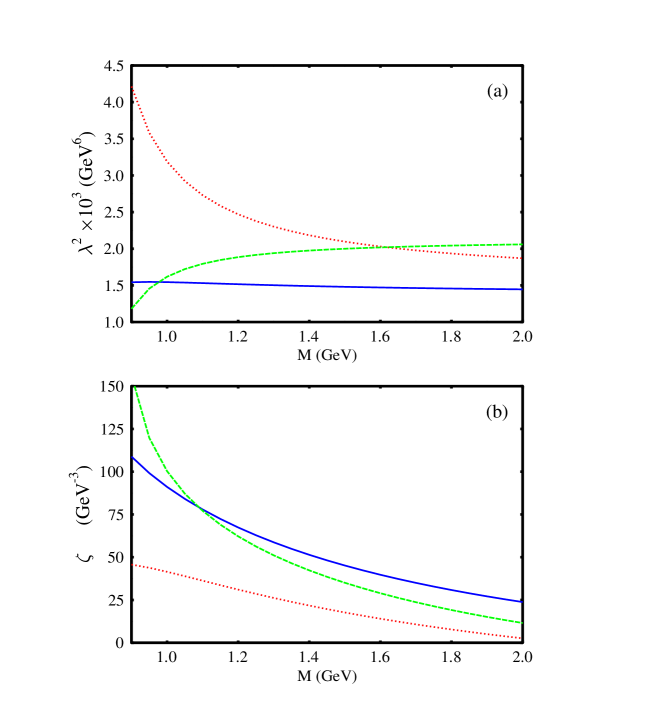
FIG. 2.: Plot of $\lambda^{2}$ and $\zeta$ as function of $M$. The solid, dotted and the dashed graphs correspond to the values (1.6, 0.3),  (1.6, 0.4),  and (1.8, 0.2) respectively for the set $(W,f)$.

V Discussion

Instead of assuming an ansatz for the two-point function, as is usually done in the literature, we have calculated it in chiral perturbation theory. To one loop, the coupling constants appearing at the vertices in Feynman graphs are all known, except for $\zeta$ arising from the vertex $\eta\rightarrow({\bar{\psi}}\psi)\psi$. We determine it from the sum rules.

As we saw at the end of Sec.III, the four-nucleon couplings lead to too big a mass shift (self-energy) of the nucleon in normal nuclear matter. It is related to the fact that the formulation of chiral perturbation theory for the two-nucleon system faces a problem, due to the proximity of the virtual or bound states to the theshold of $N\!N$ scattering [17]. It makes the effective coupling constants rather large. Further, when multiplied by $\overline{n}$ for normal nuclear matter, these are still too large for the one-loop result to be valid [21]. A resummation of the loop diagrams with these vertices is supposedly needed [26].

We must, however, point out that this breakdown of the one-loop result in normal nuclear matter does not prevent us from using this four-nucleon coupling for writing our sum rules. The point here is that we are not working in normal nuclear matter. All we need is the validity of an expansion of the two-point function in powers of $\overline{n}$ for sufficiently small $\overline{n}$. Since any resummation can only alter coefficients of terms quadratic and higher in $\overline{n}$, our use of the coefficient of $\overline{n}$ to one loop remains valid.

Our calculation does not support an assumption in the popular ansatz for the two-point function, namely that it can be well-approximated by the (dressed) nucleon pole term and an integral over the high energy region. We find that each Feynman graph, besides contributing possibly to the pole, also contributes an integral over the low energy region, which is not accounted for by the ansatz. Also there are no density dependent discontinuities of the amplituide for negative energy in nuclear medium. Hence the variable to write the dispersion integrals is $E$ and not $E^{2}$.

Finally we suggest a different use of the sum rules. There is a tendency in the literature to try to predict the nucleon self-energy from the sum rules. Indeed, this is in accordance with the works on the vacuum sum rules, where these are used to find the masses and the couplings of the single particles communicating with the currents in the two-point functions. However, it appears to us that the sum rules in the medium, as we have written, may be utilised more profitably to find the condensates in the medium.

A way to carry out such a program would be to extend the sum rules to non-zero external three-momenta $\vec{q}$. Here we retain the different four-quark operators as such, without invoking factorization. With the additional variable $\vec{q}\,^{2}$ at hand, it should be possible to extract numerical values for these oprator condensates in nuclear medium. These values may then be compared with model calculations [27].

REFERENCES

- [1] M.A. Shifman, A.I. Vainshtein and V.I. Zakharov, Nucl. Phys. B 147, 385 (1979). For a collection of original papers and comments, see Vacuum Structure and QCD Sum Rules, edited by M.A. Shifman (North Holland, Amsterdam, 1992). See also S. Narison, QCD Spectral Sum Rules (World Scientific, Singapore, 1989).
- [2] T. Hatsuda, Y. Koike and S.H. Lee, Nucl. Phys. B 394, 221 (1993) and references cited therein.
- [3] T.D. Cohen, R.J. Furnstahl, D.K. Griegel and X. Jin, Prog. Part. Nucl. Phys. 35, 221 (1995); E.G. Drukarev, M.G. Ryskin and V.A. Sadovnikova, ibid., 47, 73 (2001).
- [4] A.I. Bochkarev and M.E. Shaposhnikov, Nucl. Phys. B 268, 220 (1986).
- [5] H. Leutwyler and A.V. Smilga, Nucl. Phys. B 342, 302 (1990).
- [6] Y. Koike, Phys. Rev. D 48, 2313 (1993).
- [7] S. Mallik and S. Sarkar, Phys. Rev. D 65, 016002 (2002).
- [8] S. Mallik and S. Sarkar, Phys. Rev. D 66, 056008 (2002).
- [9] E.G. Drukarev and E.M. Levin, JETP Lett. 48, 338 (1988); Sov. Phys. JETP, 68, 680 (1989).
- [10] X. Jin, T.D. Cohen, R.J. Furnstahl and D.K. Griegel, Phys. Rev. C 47, 2882 (1992).
- [11] B.L. Ioffe, Nucl. Phys. B 188, 317 (1981); Y. Chung, H.G. Dosch, M. Kremer and D. Schall, Nucl. Phys. B 197, 55 (1982).
- [12] B.L. Ioffe, Z. Phys. C 18, 67 (1983).
- [13] For a review see N.P. Landsmann and Ch. G. van Weert, Phys. Rep. 145, 141 (1987).
- [14] R.L. Kobes, G.W. Semenoff and N. Weiss, Z. Phys. C 29, 371 (1985).
- [15] J. Gasser and H. Leutwyler, Ann. Phys. 158, 142 (1984); Nucl. Phys. 250, 465 (1985).
- [16] J. Gasser, M.E. Sainio and A. Svarc, Nucl. Phys. B 307, 779 (1988); J. Gasser, H. Leutwyler, M.P. Locher and M.E. Sainio, Phys. Lett. B 213, 85 (1988).
- [17] S. Weinberg, Phys. Lett. B 251, 288 (1990); Nucl. Phys. B 363, 3 (1991); Phys. Lett. B 295, 114 (1992).
- [18] R.P. Haddock, R.M. Salter, Jr., M. Zeller, J.B. Czirr and D.R. Nygren, Phys. Rev. Lett. 14, 318 (1965); H.P. Noyes, Phys. Rev. 130, 2025 (1963).
- [19] C. Ordonez, L. Ray and U. van Kolck, Phys. Rev. C 53, 2086 (1996).
- [20] A. Bohr and B.R. Mottelson, Nuclear Structure, vol I (W.A. Benjamin, Inc., New York, 1969).
- [21] D, Montano, D.D. Politzer and M.B. Wise, Nucl. Phys. B 375, 507 (1992).
- [22] H.A. Weldon, Phys. Rev. D 28, 2007 (1983).
- [23] R. Brockmann and R. Machleidt, Phys. Rev. C 42, 1965 (1990). See also S. Mallik, A. Nyffeler, M.C.M. Rentmeester and S. Sarkar, nucl-th/0407038, to be published in Eur. J. Phys. A .
- [24] J. Gasser, H. Leutwyler and M.E. Sainio, Phys. Lett. B 253, 252 (1991).
- [25] A.D. Martin, R.G. Roberts, W.J. Stirling and R.S. Thorne, Eur. Phys. J. C 4, 463 (1998).
- [26] D.B. Kaplan, M.J. Savage and M.B. Wise, Nucl. Phys. B 534, 329 (1998).
- [27] V.E. Lyubovitskij, P. Wang, Th. Gutsche and A. Faessler, Phys. Rev. C 66, 055204 (2002) and references cited therein.