Hadron resonance probes of QGP

Abstract

We discuss the indirect and direct role of the short-lived resonances as probes of QGP freeze-out process. The indirect effect is the distortion of stable single particle yields and spectra by contributions of decaying resonances, which alter significantly the parameters obtained in fits to experimental data. We than discuss the direct observation of short-lived resonances as a probe of post-hadronization dynamics allowing to distinguish between different hadronization models.

I Introduction

We would like to understand the dynamics of quark-gluon plasma (QGP) phase breakup into individual hadrons and show here how this can be done using hadron resonances. To convert QGP into hadrons we employ the Fermi statistical model of particle production Fer50 ; Pom51 ; Lan53 ; Hag65 ; CooperFrye ; jansbook . This approach has been used extensively in the field of relativistic heavy ion collisions. Particle abundances and spectra both at Super Proton Synchrotron (SPS)  PBM99 ; NA57 ; becattini ; van-leeuwen ; ourspspaper ; sqm2001 ; PBM01 and Relativistic Heavy Ion Collider (RHIC)  burward-hoy ; castillo ; PBMRHIC ; bugaev_freeze ; florkowski ; rafelski2002 energies have been analyzed in this way. In all this studies one relies on presence of a distinct condition in temperature at which the rate of particle interactions goes to zero (freeze-out). The HBT fasthbt measurements and the success of statistical models suggest that the freeze-out process at SPS and RHIC energies is indeed much faster than previously expected, being close to the explosive hadronization limit of instantaneous emission and negligible post-emission interactions sudden .

The obvious way to test this model experimentally is to obtain experimental measure of the time lapse between hadronization and end of hadron-hadron interaction. While HBT has always been considered the ideal probe to do it, the fact that hydrodynamic models at present fail to describe HBT data heinzkolb , together with the problems associated with emission from an interacting gas with non-zero mean free path wrongHBT make the search for a different probe of freeze-out time necessary. Since hadronization is a fast process, resonance decay products have an appreciable chance of escaping without rescattering and thus resonance yields can be measured directly, and in an analysis of these results one can obtain information about hadronization dynamics.

Therefore we consider direct detection of hadronic short-lived resonances as an alternative probe of freeze-out dynamics. We find that the short-lived resonances, detectable through invariant mass reconstruction fachini ; vanburen ; markert ; friese are natural candidates for freeze-out diagnostics since their lifetime is comparable to the hadronization timescale and the lifetime of the interacting HG. Resonances usually have the same quark numbers as light particles, making their yield compared to the light particle independent of chemical potential. The rich variety of detected resonances vanburen includes particles with very different masses and widths, allowing us to probe both production temperatures and interaction lifetimes in detail. Fig. 1 shows what percentage of observed light particles comes from the decays of heavier resonances (quite a few of them experimentally observable). As can be seen in figure 1 this resonance contribution is significant, and varies appreciably with both particle type and temperature.

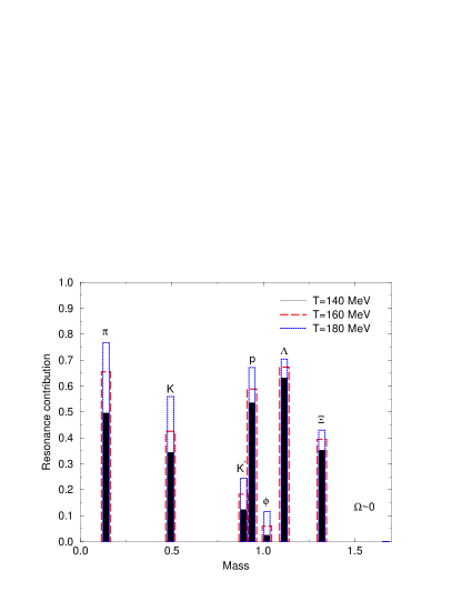
Figure 1: (Color online) Relative resonances contribution to individual stable hadrons for three particle freeze-out temperatures.

II Resonance influence on particle spectra

Statistical hadronization model assumes that, in the rest-frame with respect to collective matter flow, particle spectra are given by the (entropy maximizing) Boltzmann spectrum. In addition, the phase space occupancy by particles is affected by the space-time geometry of the particle emission surface. The particle spectrum in the laboratory rest frame is given by,

$$\frac{d^{2}N}{dm_{T}dy} \propto \left(1-\frac{\vec{v}_{f}^{\,-1}\cdot\vec{p}}{E}\right)\,m_{T}\cosh y\,e^{-\gamma\frac{E}{T}\left(1-\frac{\vec{v}\cdot\vec{p}}{E}\right)}\,,\quad$$ (1)

$$\gamma = 1/\sqrt{1-v^{2}}.$$ (2)

Taking feed-down from resonances into account can be tedious numerical task. To simplify the situation we assume that, in a decay of the form,

$$R\rightarrow 1+2+...,$$ (3)

dynamical effects in the decay average out over a statistical sample of many resonances. In other words, in the rest frame comoving with the “average” resonance, the distribution of the decay products will be isotropic. If more than two body decays are considered, this calculation becomes more involved phasespace . For the general N-body case, evaluation is better left to Monte Carlo methods mambo .

The rate of particles of type 1 (as in eq. (3)) produced with momentum $\vec{p^{*}_{1}}$ in the frame at rest w.r.t. the resonance will then be given by the Lorenz invariant phase space factor of a particle of mass $M_{1}$ and momentum $\vec{p^{*}_{1}}$ within a system with center of mass energy equal to the resonance mass $M_{R}$,

$$\frac{d^{3}N_{1}}{d^{3}p^{*}_{1}}=b\int\prod_{i=2}^{n}\frac{d^{3}p^{*}_{i}}{2E^{*}_{i}}\delta(\sum_{i=2}^{N}p^{*}_{i}-p^{*}_{1})\delta(\sum_{i=2}^{N}E^{*}_{i}-E^{*}_{1}-M_{R}).$$ (4)

Here $b$ is the branching ratio of the considered decay channel. To obtain laboratory spectrum we need to change coordinates from the resonance’s rest frame $(p^{*},E^{*})$ to the lab frame $(p,E)$.

In the case of the 2-body decay $p^{*},E^{*}$ are fixed by the masses of the decay products,

$$E^{*}_{1}=\frac{1}{2M_{R}}(M_{R}^{2}-m_{1}^{2}-m_{2}^{2}),$$ (5)

$$p^{*}_{1}=-p^{*}_{2}=\sqrt{E_{1}^{*2}-m_{1}^{2}}.$$ (6)

Putting the constraints in eq. (5) into eq. (4) one gets, after some algebra resonances

$$\frac{dN}{d{m^{2}_{T1}}dy_{1}}=\frac{b}{4\pi p^{*}_{1}}\int_{Y-}^{Y+}\!\!\!dY_{1}\!\!\int_{M_{T}-}^{M_{T}+}\!\!\!dM_{T1}^{2}J\frac{d^{2}N_{R}}{dM_{TR}^{2}dY_{R}},$$ (7)

$$\noindent J=\frac{M_{R}}{\sqrt{P_{TR}^{2}p_{T1}^{2}-(M_{R}E^{*}_{R}-M_{TR}m_{T1}\cosh\Delta Y)^{2}}},$$ (8)

$$\Delta Y=Y_{R}-y_{1}.$$ (9)

$J$ is the Jacobian of the transformation from the resonance rest frame to the lab frame, and the limits of the kinematically allowed integration region are:

$$\ Y_{\pm}=y_{1}\pm\sinh^{-1}\left(\frac{p^{*}_{1}}{m_{T1}}\right)$$

$$\ M_{T}^{\pm}=M_{R}\frac{E^{*}_{R}m_{T1}\cosh(\Delta Y)\pm p_{T1}\sqrt{p^{*2}_{1}-m_{T1}^{2}\sinh^{2}(\Delta Y)}}{m_{T1}^{2}\sinh^{2}(\Delta Y)+m^{2}_{1}}$$

This calculation assumes resonances are produced through the same statistical model which is fitted to the momenta of the daughter particles, and their decay products reach the detector with no further interaction. How the data is described in this approach is seen in figure 2 for the most peripheral, and the most central reaction bin. Solid lines show the no-rescattering fit quality for particle spectra. When rescattering of the decay products is important the shape of the spectra are as if there were no resonance decays. This case is presented by dashed lines in figure 2. Clearly there is a much more physically significant spectra fit possible if we allow that hadron resonances are present and their decay products do not rescatter.

Figure 2: $\chi^{2}$ profile for a fit to WA97 $K_{S},\Lambda,\overline{\Lambda},\Xi,\overline{\Xi},\Omega,\overline{\Omega}$ data at 158 GeV wa97 . Solid line: resonance decays included. Dotted line: resonances reequilibrated.

Inclusion of resonances in the spectral fit requires no extra degrees of freedom, and the improvement of $\chi^{2}$ of the fit of the SPS hyperon spectra seen in figure 2 wa97 convincingly favors models in which resonances are present within the fireball in the abundances predicted by a single freeze-out temperature model. Not including spectral contributions of resonances raises the $\chi^{2}$ by a factor of 3 and removes the $\chi^{2}$ minimum’s significance. We have not yet found a particle type for which consideration of resonances does not lower the $\chi^{2}$. Moreover, we find considering possible mass or width shift that such effects significantly increase the $\chi^{2}$ ourspspaper , and thus there is another evidence that rescattering, which usually shifts masses and widths shuryak , is minimal.

III Resonance yields as probe of hadronization dynamics

The fact that resonances have been found to give the contribution to particle spectra predicted by the statistical model has motivated the direct search of resonances through invariant mass reconstruction fachini ; vanburen ; markert ; friese . It has been found that while statistical models are able to fit the $K^{*}/K$ ratio within error PBMRHIC , the $\Lambda(1520)$ is strongly suppressed at both SPS and RHIC energies markert . This puzzling result suggests that both emission temperature and re-scattering might make a significant contribution to resonance abundance, and their roles need to be disentangles. This is possible by considering abundances of two resonances with different masses (which constrains the temperature) as well as lifetimes (which probes the role of non-equilibrium in-medium effects, i.e. rescattering).

To obtain a quantitative estimate, we have calculated the ratios of $(K^{*}+\overline{K^{*}})/K_{S}$ and $\Lambda(1520)/\Lambda$ using the statistical model. In both cases chemical potential corrections are negligible since the particle’s chemical composition is the same and thus we have:

$$\frac{N^{*}}{N+N^{*}} = \frac{n(m^{*},T)}{n(m^{*},T)+n(m,T)},$$ (10)

$$n(m,T) = m^{2}TK_{2}\left(\frac{m}{T}\right).$$ (11)

We then evolved in time the ratios using a model which combines an average rescattering cross-section with dilution due to a constant collective expansion. In this model, the initial resonances decay with width $\Gamma$ through the process $N^{*}\rightarrow D$. Their decay products $D$ ($D(t=0)=0$) then undergo rescattering at a rate proportional to the medium’s density as well as the average rescattering rate. The final evolution equations then are

$$\frac{dN^{*}}{dt} = -\Gamma N^{*}+R,$$ (12)

$$\frac{dD}{dt} = \Gamma N^{*}-D\sum_{j}\langle\sigma_{Dj}v_{Dj}\rangle\rho_{j}\left(\frac{R_{0}}{R_{0}+vt}\right)^{3}.$$ (13)

$v$ is the expansion velocity, $R_{0}$ is the hadronization radius, $\rho_{j}=n_{j}(m_{j},T)$ the initial hadron gas particle density and $\langle\sigma_{Dj}v_{Dj}\rangle$ is the particle specific average flow and interaction cross-section.

In this calculation, we have neglected the regeneration term $R\propto\langle\sigma_{Di}^{INEL}v_{Di}\rangle\rho_{i}$, since detectable regenerated resonances need to be real (close to mass-shell) particles. Figure 3 shows how the ratios of $\Sigma^{*}/\Lambda$ and $K^{*}/K$ evolve with varying hadronization time within this model.

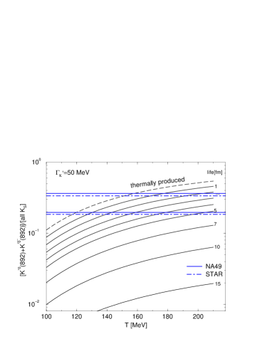
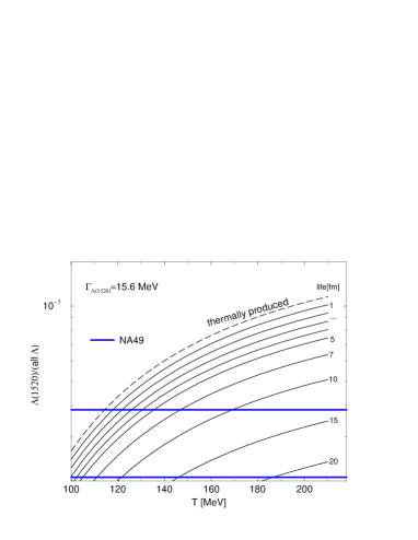
Figure 3: Observable relative resonance yields as a function of temperature for a given length in time of interacting hadron gas phase. Horizontal and vertical lines give experimental results.

It therefore becomes apparent that measuring two such ratios simultaneously gives both the hadronization temperature and the time during which rescattering is a significant effect. Figure 4 shows the application of this method to $K^{*},\Lambda(1520)$ and $\Sigma^{*}$.

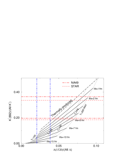
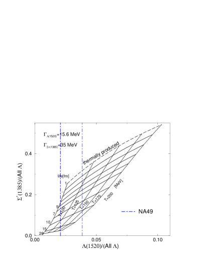
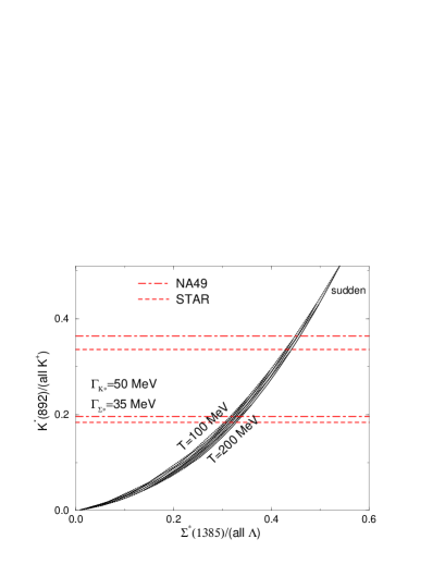
Figure 4: Projected combined relative yield diagrams over a mesh of temperature and lifespan. Horizontal and vertical lines give experimental results.

The special role of $\Lambda(1520)$ suppression is evident. $\Lambda(1520)$ is a very peculiar resonance, since unlike the $K^{*}$ and $\Sigma^{*}$ it’s extra spin is believed to originate from inter-quark orbital angular momentum (L=2). It is therefore particularly susceptible to in-medium effects which suppress it’s yield or enhance it’s width JRPRC ; pasi . If this is the case, our model is able to account for existing observational data and makes definite predictions for the measured $\Sigma^{*}$ abundance.

IV Resonance spectra as direct probe of freeze-out dynamics

The near-independence of resonances on chemical potential makes their direct detection a powerful tool for examining further aspects of freeze-out dynamics. It is apparent from the previous section that the ratio of the resonance to the daughter particle with the same number of quarks is extremely sensitive to freeze-out temperature.

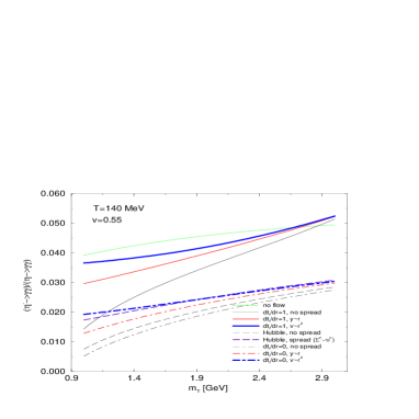
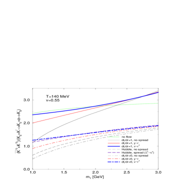
Figure 5: Spectral ratios as function of $m_{\bot}$ for an array of freeze-out surface conditions.

If the $m_{\bot}$ dependence of this ratio can be observed further freeze-out parameters can be extracted statres . For a purely thermal source, in which

$$\frac{dN}{dm_{\bot}}\propto g\cosh(y)m_{\bot}^{2}e^{-\frac{m_{\bot}}{T}}$$ (14)

the observed resonance ratio should be a step function, with $N^{*}/N=0$ for $m_{\bot}<m^{*}$ and the ratio of degeneracies for the resonance $g^{*}/g$ for $m_{\bot}>m^{*}$.

However, a non-trivial flow profile and emission geometry can significantly change this dependency. For this reason, this ratio is an extremely sensitive probe of both flow profile (the transverse flow as function of the radius) and hadronization dynamics (how emission time varies with space, parametrized by $\vec{v}_{f}$ in eq. 1). Figure 5 shows this ratio (calculated by dividing two expressions of the form of eq. 1 but different masses) done for $\eta^{\prime}\rightarrow\gamma\gamma/\eta\rightarrow\gamma\gamma$ and $(K^{*}+\overline{K^{*}})/K_{S}$. It is apparent that this measurement is indeed a sensitive probe of freeze-out dynamics and flow. Moreover, flow effects are separated from freeze-out dynamics, something which “normal” hadronic spectra can not do effectively comparison .

In conclusion, we have presented here an outline of the use of resonances as diagnostic tools in the study of freeze-out dynamics. We have shown that statistical fits to particle spectra require an admixture of resonances consistent with thermal predictions, which strongly suggests negligible post-hadronization rescattering dynamics. We have described how the study of resonances yields and spectra can yield the hadronization temperature, the timescale of thermal freeze-out, and the freeze-out geometry dynamics. We expect these models to be constrained and developed further as resonance experimental data becomes more precise.