A comprehensive treatment of electromagnetic interactions and the three-body spectator equations

Abstract

We present a general derivation the three-body spectator (Gross) equations and the corresponding electromagnetic currents. As in previous paper on two-body systems, the wave equations and currents are derived from those for Bethe-Salpeter equation with the help of algebraic method using a concise matrix notation. The three-body interactions and currents introduced by the transition to the spectator approach are isolated and the matrix elements of the e.m. current are presented in detail for system of three indistinguishable particles, namely for elastic scattering and for two and three body break-up. The general expressions are reduced to the one-boson-exchange approximation to make contact with previous work. The method is general in that it does not rely on introduction of the electromagnetic interaction with the help of the minimal replacement. It would therefore work also for other external fields.

I Introduction

Exposing few nucleon systems to medium energy ($\sim 1$GeV) electromagnetic probes requires a relativistic description of initial and final states as well as of the reaction mechanism. The relativistic effects are usually included in perturbative way vc , but even at leading order one has to include large number of terms into NN potential and electromagnetic current, while the convergence of the series in $v/c\sim p/m$ becomes questionable. The conceptually cleaner alternative is to start from an explicitly covariant formulation. A number of covariant techniques has been introduced and studied extensively for the case of the simplest two nucleon system, in particular in calculations of the elastic e.m.  deuteron form factors GVO and in deuteron electro- and photodisintegration GGr .

In the present paper we adopt the spectator (or Gross) quasipotential approach spectator ; Gr82 . It reduces four dimensional integrals over loop momenta to their more treatable three dimensional form in explicitly covariant way by picking up the poles of nucleon propagators. This simplifies an analytic structure of dynamic equations and leads to closer approximation to full result compared to the Bethe-Salpeter ladder approximation. A set of realistic one-boson-exchange potentials were constructed within the formalism, giving a fair fit to NN scattering data and deuteron properties NNspect . It was found that the model gives very good description of the elastic deuteron form factors GVO ; deutff . Three nucleon spectator equation with those realistic potentials was solved by Stadler and Gross sg and the normalization condition for the 3N bound state amplitudes was derived norm . The first calculation of electromagnetic break-up of 3N bound state are in progress.

In order to calculate this process it is necessary to determine the correct effective electromagnetic current operator to be used with the three-body spectator equation. So far this problem has been approached in two ways. The first of these is the elegant method of Kvinikhidze and Blankleider kb97 ; kb97II ; kb99 that gauges the integral equations which describe the strongly interacting system in order to obtain the electromagnetic current matrix elements for various processes. The second approach is that of Gross, Stadler and Peña Gr04 which uses an approach based on a diagrammatic description of the three-body system and relies heavily on the gauging approach. These two approaches lead to identical results once differences in organization are accounted for. In both of these papers certain assumptions are inherent in the results that are presented Gr04 . In both cases, no explicit three-body forces are included and the results implicitly assume that the interaction kernels are given by the one-boson-exchange approximation.

In a previous paper 2Ncur we pursued a different strategy to obtain a general derivation of the e.m. currents for the two-body Gross equation. The starting point was the organization of the corresponding Feynman amplitudes into 2N Bethe-Salpeter equation and factorization of five point Green function (with the external e.m. field). The spectator equations were then obtained by separating the propagator of one of the two particles into a piece containing only the on-shell positive-energy contribution and a remainder. The Bethe-Salpeter amplitudes are then rearranged into integral equations which contain only the on-shell propagator and a quasipotential equation which sums all of the off-shell contributions. The electromagnetic current consistent with this rearrangement was derived with the help of operator algebra, which defines the products of singular operators and represents an useful shortcut alternative to pole analysis of the Feynman diagrams. We have shown that this definition is consistent with gauge invariance when a necessary truncation of the strong kernel is applied in any finite order of quasipotential decomposition and in a number of meson exchanges involved. The main aim of the present paper is to extend this treatment to 3N spectator equation and to derive general expressions for electromagnetic matrix elements needed for the future application to actual calculation of the electromagnetic properties of relativistic three nucleon systems.

For convenience, Sec. II contains a brief review of the application of this approach to the two-body system.

The starting point of the analogous development for three-body systems is a description of the three-body Bethe-Salpeter amplitudes given by four-dimensional integral equations that iterate kernels consisting of all three-body irreducible contributions to the six-point function. The currents consistent with these kernels can be obtained either by attaching a photon to all internal particle propagators in a diagrammatic representation the kernels, or by use of the gauging method kb99 . Section III contains a review of the three-body Bethe-Salpeter equations and current including contributions from two- and three-body kernels and currents. Since the three-body spectator equations are defined only for three identical particles a discussion of the three-body equations for identical particles is given in Sec. IIIC. Before using our approach to obtain the spectator equations, it is convenient to use the symmetry of the various Faddeev amplitudes to limit the number of channels that explicitly appear in the equations. We found that it is most convenient to do this in the context of a matrix representation of the channel space. Appendix A describes the matrix method for three distinguishable particles and Appendix B describes the case of identical particles and show how to reduce the problem to two channels.

Section IV applies the operator technique to the two-dimensional matrix representation of the Bethe-Salpeter equation to obtain the corresponding spectator equations for the t-matrix and wave functions, and obtains an expression for the corresponding effective current operator. Some care is taken to separate two-body quasipotential and scattering matrix contributions from three-body contributions that are generated by the transformation from the Bethe-Salpeter to the spectator equations. These contributions can occur even if there are no explicit three-body Bethe-Salpeter interactions.

In Sec. V we show how the general expressions obtained in Sec. IV can be reduced to the case of the one-boson-exchange approximation for the Bethe-Salpeter kernels and currents. This gives results identical to those of Gross, Stadler and Peña; and, by extension, to those of Kvinikhidze and Blankleider.

II Review of the Two-body Equations

The motivation for the arguments that we present below for constructing the three-body electromagnetic current matrix elements for the three-body spectator equation is best illustrated by providing an outline of the arguments that appeared in our previous paper 2Ncur for obtaining the equivalent expressions for the two-body spectator equation.

First consider the two-body Bethe-Salpeter equation for two particles interacting by the exchange of a boson. Examination of all of the diagrams contributing to the two-body t-matrix (the four-point vertex function) allows to show that the sum of all contributions to the t-matrix can be represented by an integral equation of the form

$$M=V-VG_{BS}M\,,$$ (1)

where the kernel of the equation $V$ is the sum of all two-body irreducible diagrams, and where $G_{BS}=-iG_{1}G_{2}$ is the free two-body Bethe-Salpeter propagator. The formalism reviewed in this section and further developed in this paper for three particle systems is restricted to the energies below particle production threshold. That is, the propagation of the constituents is approximated by free Green’s functions with the physical mass and the phenomenologically dressed interaction vertices are assumed, i.e., explicit loops dressing two- and three-point Green’s functions and their renormalization are not considered. The two-body interacting propagator (four-point propagator) can then be written as

$${\cal G}=G_{BS}-G_{BS}MG_{BS}=G_{BS}-G_{BS}V{\cal G}=G_{BS}-{\cal G}VG_{BS}\,.$$ (2)

This propagator contains all of the information about the two-body system and the bound and scattering states wave functions can be obtained from the singularities of this propagator. By looking for sub-threshold poles in the propagator the bound state Bethe-Salpeter wave function can be determined to be

$$\left|\psi\right>=G_{BS}\left|\Gamma\right>\,,$$ (3)

where $\left|\Gamma\right>$ is the bound-state Bethe-Salpeter vertex function which satisfies the equation

$$\left|\Gamma\right>=-VG_{BS}\left|\Gamma\right>\,.$$ (4)

The pole in the propagator associated with the two incoming particles being on mass shell gives the scattering wave function with outgoing wave boundary conditions

$$\left|\psi^{(+)}\right>=\left(1-G_{BS}M\right)\left|\bm{p}_{1},s_{1};\bm{p}_{2},s_{2}\right>$$ (5)

and the corresponding pole for the outgoing particles gives the conjugate scattering wave function with incoming wave boundary conditions

$$\left<\psi^{(-)}\right|=\left<\bm{p}_{1},s_{1};\bm{p}_{2},s_{2}\right|\left(1-MG_{BS}\right)\,.$$ (6)

All of the wave functions satisfy the wave equation

$${\cal G}^{-1}\left|\psi\right>=0\,.$$ (7)

The relationship of the two-body interacting propagator to the wave functions implies that we can obtain all of the necessary information concerning the electromagnetic currents for this system in one-photon-exchange approximation by examining all Feynman diagrams contributing to a five-point propagator with one photon leg and four interacting particle legs. This five-point propagator can be written as

$${\cal G}^{\mu}=-\cal{G}J^{\mu}\cal{G}$$ (8)

by defining the current operator

$$J^{\mu}=iJ_{1}^{\mu}G^{-1}_{2}+iJ_{2}^{\mu}G^{-1}_{1}+J^{(2)\mu}_{12}\,,$$ (9)

where $J^{\mu}_{i}$ is the one-body current operator for particle $i$ and $J^{(2)\mu}_{12}$ is the two-body current composed of all two-body irreducible diagrams involving the absorption of a photon. Any current matrix element can then be obtained by picking out the poles in the initial and final interacting propagators corresponding to either bound or scattering states. This current operator satisfies the Ward-Takahashi identity

$$q_{\mu}J^{\mu}=\left[e_{1}(q)+e_{2}(q),{\cal G}^{-1}\right]\,,$$ (10)

where $q_{\mu}$ is the photon momentum, $e_{t}(q)$ is the product of the charge $e_{t}$ for particle $t$ (which might be an operator in isospin space) and a four-momentum shift operator defined such that

$$\left<p^{\prime}_{t}|e_{t}(q)|p_{t}\right>=e_{t}(2\pi)^{4}\delta^{4}(p^{\prime}_{t}-p_{t}-q)\,.$$ (11)

This along with the wave equation guarantees that the current will be conserved for all possible two-body matrix elements.

The spectator or Gross equation (for distinguishable particles) can be obtained from the Bethe-Salpeter equation by substituting a two-body noninteracting propagator $g_{1}$ with particle 1 on mass shell for the Bethe-Salpeter propagator $G_{BS}$. The t-matrix will remain unchanged if it is written as a pair of coupled equations

$$M=U-Ug_{1}M$$ (12)

and

$$U=V-V\Delta g_{1}U\,,$$ (13)

where the new kernel $U$ is called the quasipotential and $\Delta g_{1}=G_{BS}-g_{1}$.

In 2Ncur it was shown that there exist a set of relationships for the spectator scattering matrix, propagators, wave functions and currents which are of the same form as those given above for the Bethe-Salpeter equation and that an effective current operator can be derived, satisfying a Ward-Takahashi identity which leads to current conservation when used with the spectator wave functions. For identical particles the formalism can be represented in a compact and transparent matrix notation.

We will now show that a similar organization can be obtained for the three-body Bethe-Salpeter and Gross equations. We will do this assuming that there may be explicit three-body interactions in addition to two-body interactions and will obtain expressions for the three-body Gross equations and effective currents which can be expanded to arbitrary order.

III Three-body Bethe-Salpeter Equation

III.1 Three-body t-matrix and wave functions

The three-body Bethe-Salpeter equation can be motivated in much the same way as in the two-body case. Examining the Feynman diagrams contributing to the three-body t-matrix it is possible to separate them into two categories, three-body reducible and irreducible diagrams. The irreducible diagrams fall into two classes, those where only two of the three particles are interacting and those where all three particles are interacting. The sum of all irreducible diagrams can then be written as

$${\cal V}=V^{0}+\sum_{i=1}^{3}V^{i}iG^{-1}_{i}={\cal V}^{0}+\sum_{i=1}^{3}{\cal V}^{i}\,,$$ (14)

where $V^{0}$ is the sum of all three-body irreducible diagrams where all three particles are interacting and $V^{i}$ is the sum of all diagrams where only particles $j$ and $k$ (with $j\neq k\neq i$) are interacting. That is $V^{0}$ is a three-body interaction and $V^{i}$ is a two-body interaction. The three-body t-matrix can then be written as

$${\cal T}={\cal V}-{\cal V}G^{0}_{BS}{\cal T}={\cal V}-{\cal T}G^{0}_{BS}{\cal V}\,,$$ (15)

where the three-particle free propagator in terms of the individual propagators reads $G^{0}_{BS}=-G_{1}G_{2}G_{3}$.

The three-body Bethe-Salpeter six-point Green function is then given as:

$${\cal G} = G^{0}_{BS}-G^{0}_{BS}{\cal V}{\cal G}=G^{0}_{BS}-{\cal G}{\cal V}G^{0}_{BS}$$ (16)

$$= G^{0}_{BS}-G^{0}_{BS}{\cal T}G^{0}_{BS}\,.$$

Obviously, the inverse three-body propagator is

$${\cal G}^{-1}=(G^{0}_{BS})^{-1}+{\cal V}\,.$$ (17)

It is convenient to introduce the Faddeev decomposition of the full t-matrix into subamplitudes ${\cal T}^{ij}$,

$${\cal T}=\sum_{i,j=0}^{3}{\cal T}^{ij}\,,$$ (18)

where the indices $i$ and $j$ characterize the subamplitudes according to the character of the last and first interactions; ie., for $i\neq 0$ ($j\neq 0$) , the particles $i$ ($j$) are not taking part in the last (first) interaction, $i=0$ ($j=0$) means that the last (first) interaction is genuine three-particle interaction. The subamplitudes ${\cal T}^{ij}$ satisfy the following integral equations (see also ref. norm )

$${\cal T}^{ij}={\cal V}^{i}\delta_{ij}-{\cal V}^{i}G^{0}_{BS}\sum_{k=0}^{3}{\cal T}^{kj}\,.$$ (19)

For numerical solution it is more appropriate to re-write these equations in terms of two-body and three-body t-matrices which subsume the corresponding interaction kernels sg :

$$M^{i}=V^{i}-V^{i}G^{i}_{BS}M^{i}\,,$$ (20)

where $M^{i}$ is the two-body scattering matrix and $G^{i}_{BS}=-iG_{j}G_{k}=iG^{-1}_{i}G^{0}_{BS}$; and

$$M^{0}=V^{0}-V^{0}G^{0}_{BS}M^{0}\,,$$ (21)

iterates to all orders the three-body interaction . The subamplitudes for three-body Bethe-Salpeter equation for distinguishable particles can be written as

$${\cal T}^{ij} = M^{i}iG^{-1}_{i}\delta_{ij}-M^{i}G^{i}_{BS}\sum_{k=0}^{3}B_{ik}{\cal T}^{kj}$$ (22)

$$= {\cal M}^{i}\delta_{ij}-{\cal M}^{i}G^{0}_{BS}\sum_{k=0}^{3}B_{ik}{\cal T}^{kj}\,,$$

where $B_{ik}=1-\delta_{ik}$ and ${\cal M}^{i}$ are defined in terms of $M^{i}$ as in eq. (14).

As in the two-body case, the three-body Bethe-Salpeter wave functions can be obtained by examining the residues of poles in the interacting three-body propagator. The wave function for a three-body bound state with mass $M_{B}$ is related to the residue of the propagator at a pole corresponding to $P^{2}=M_{B}^{2}$, where $P$ is the total momentum of the three-body system. From the resolved form of the propagator, it is clear that this is due to a pole in the t-matrix. The three-body bound state vertex function is related to the residue of the t-matrix at this pole so that the t-matrix reads

$${\cal T}=-\frac{\left|\Gamma\right>\left<\Gamma\right|}{M_{2}^{2}-P^{2}}+{\cal R}\,.$$ (23)

Using this in the t-matrix equation, the vertex function can be shown to satisfy the equation

$$\left|\Gamma\right>=-{\cal V}G^{0}_{BS}\left|\Gamma\right>\,.$$ (24)

The interacting three-body propagator can be written as

$${\cal G}=\frac{G^{0}_{BS}\left|\Gamma\right>\left<\Gamma\right|G^{0}_{BS}}{M_{2}^{2}-P^{2}}+G^{0}_{BS}-G^{0}_{BS}{\cal R}G^{0}_{BS}\,.$$ (25)

The bound-state wave function is defined as

$$|\Psi>=G^{0}_{BS}\left|\Gamma\right>\,,$$ (26)

which satisfies the wave equation

$${\cal G}^{-1}|\Psi>=0\,.$$ (27)

The bound state vertex and wave functions are decomposed into their Faddeev components:

$$|\Gamma> = \sum_{i=0}^{3}|\Gamma^{i}>\,,$$ (28)

$$|\Psi> = \sum_{i=0}^{3}|\Psi^{i}>\,,$$ (29)

defined by dynamical equations

$$|\Gamma^{i}> = -{\cal V}^{i}G^{0}_{BS}|\Gamma>\,,$$ (30)

$$(G^{0}_{BS})^{-1}\,|\Psi^{i}> = -{\cal V}^{i}|\Psi>\,,$$ (31)

where $i=0,1,2,3$.

The scattering states can be obtained from (16). Since $G^{0}_{BS}$ has poles at the on-shell masses of particles with plane-wave residues, isolating the poles for the right-hand propagators in (16) gives the three-body scattering wave function with outgoing-wave boundary conditions

$$\left|\Psi^{(+)}\right>=\left(1-G^{0}_{BS}{\cal T}\right)\left|\bm{p}_{1},s_{1};\bm{p}_{2},s_{2};\bm{p}_{3},s_{3}\right>\,,$$ (32)

while doing so for the left-hand yields the conjugate scattering wave function with incoming-wave boundary conditions.

$$\left<\Psi^{(-)}\right|=\left<\bm{p}_{1},s_{1};\bm{p}_{2},s_{2};\bm{p}_{3},s_{3}\right|\left(1-{\cal T}G^{0}_{BS}\right)\,,$$ (33)

where

$$\left|\bm{p},s\right>=\left\{\begin{array}[]{ll}u(\bm{p},s)\left|\bm{p}\right>&\quad{\rm for\ spin}=\frac{1}{2}\\ \left|\bm{p}\right>&\quad{\rm for\ spin}=0\end{array}\right.$$ (34)

The Faddeev components of the three-body scattering wave function are given by

$$\left<\Psi^{(-)i}\right|=\left<\bm{p}_{1}\bm{p}_{2}\bm{p}_{3}\right|Q_{1}Q_{2}Q_{3}\left(\frac{1}{4}-\sum_{k}{\cal T}^{ki}G^{0}_{BS}\right)\,.$$ (35)

In order to extract the scattering states where two of the particles are bound and the other is in the continuum, the propagator eq. (16) is rewritten using (22) as

$${\cal G} = G^{0}_{BS}-G^{0}_{BS}\sum_{j=0}^{3}{\cal T}^{0j}G^{0}_{BS}$$ (36)

$$-\sum_{i=1}^{3}\sum_{j=0}^{3}\left[G^{i}_{BS}{\cal M}^{i}iG_{i}G^{i}_{BS}\delta_{ij}-G^{i}_{BS}{\cal M}^{i}iG_{i}G^{i}_{BS}\sum_{k=0}^{3}B_{ik}{\cal T}^{kj}G^{0}_{BS}\right]\,.$$

The last term in this expression contains the two-body scattering matrices which have poles corresponding to the two-body bound states and can be represented by

$${\cal M}^{i}=-\frac{\left|\Gamma^{(2)i}\right>\left<\Gamma^{(2)i}\right|}{M_{2}^{2}-{P^{i}}^{2}}+{\cal R}$$ (37)

where $\left|\Gamma^{(2)i}\right>$ is the two-body bound-state vertex function for the pair of interacting particles $j$ and $k$ ($j\neq k\neq i$), $M_{2}$ is the mass of the two-body bound state and $P^{i}$ is its total momentum. This term also contains the free propagator for particle $i$. By selecting the residues of the pole for particle 1 (putting $i=1$) and the bound-state of particles 2 and 3, the conjugate state two-body scattering state with incoming-wave boundary conditions can be identified as

$$\left<\Phi^{1(-)}\right| = \left<\Gamma^{(2)1};\bm{p}_{1},s_{1}\right|G^{1}_{BS}\left[1-\sum_{k=0}^{3}\sum_{i=0}^{3}B_{1k}{\cal T}^{ki}G^{0}_{BS}\right]$$ (38)

$$= \left<\Phi^{(2)1};\bm{p}_{1},s_{1}\right|\left[1-\sum_{k=0}^{3}\sum_{i=0}^{3}B_{1k}{\cal T}^{ki}G^{0}_{BS}\right]\,,$$

$$\left<\Phi^{1(-)}\right| = \sum_{i=0}^{3}\left<\Phi^{1(-)i}\right|\,,$$ (39)

$$\left<\Phi^{1(-)i}\right| = \left<\Phi^{(2)1};\bm{p}_{1},s_{1}\right|\left[\delta_{1i}-\sum_{k\neq 1}{\cal T}^{ki}G^{0}_{BS}\right]\,.$$ (40)

A similar expression can be obtained for the wave function with outgoing-wave boundary conditions.

All of the wave functions satisfy the wave equation

$${\cal G}^{-1}|\Psi>=0\,.$$ (41)

III.2 Electromagnetic current in Bethe-Salpeter framework

The three-body Bethe-Salpeter current can be determined by considering all diagrams contributing to the seven-point function with six legs corresponding to the three incoming and outgoing particles and one photon leg. By separating the diagrams into three-particle reducible and irreducible contributions the current operator can be identified as the sum of all irreducible seven-point functions. There will be three types of contributions: one-body contributions where the photon attaches to only one of the interacting particles, two-body contributions where the photon attaches internally to a two-body interaction, and three-body contributions where the photon attaches internally to a three-body interaction.

The one-body currents are of the form

$$J^{t\mu}=-J^{\mu}_{t}G_{r}^{-1}G_{s}^{-1}\,,$$ (42)

where $t=1,2,3$, $r\neq s\neq t$ and $J^{\mu}_{t}$ is the vertex for attaching a photon to particle $t$, for which $q_{\mu}J^{\mu}_{t}=\left[e_{t}(q),G_{t}^{-1}\,\right]$. Each of these currents satisfies the Ward-Takahashi identities

$$q_{\mu}J^{t\mu}=\left[e_{t}(q),(G^{0}_{BS})^{-1}\,\right]\,.$$ (43)

As in the case of two-particle system 2Ncur ; GrossRiska , the two- and three-body currents follow from attaching a photon line to all particle lines and into momentum-dependent vertices internal to the two- and three-body Bethe-Salpeter kernels. Defining $J^{(2)\mu}_{rs}$ as the two-body current as extracted from the two-body problem and $J^{(3)\mu}$ as the completely connected three-body current, the exchange current for the three-body system can be written as

$$J^{t\mu}_{\rm ex}=\left\{\begin{array}[]{ll}J^{(2)\mu}_{rs}iG^{-1}_{t},&t=1,2,3\ \ (r\neq s\neq t)\\ J^{(3)\mu},&t=0\end{array}\right.$$ (44)

which satisfies the Ward-Takahashi identities

$$q_{\mu}J^{t\mu}_{\rm ex}=\left\{\begin{array}[]{ll}\left[e_{r}(q)+e_{s}(q),{\cal V}^{t}\right],&t=1,2,3\ \ (r\neq s\neq t)\\ \left[e_{T}(q),{\cal V}^{0}\right],&t=0\end{array}\right.$$ (45)

where $e_{T}(q)=e_{1}(q)+e_{2}(q)+e_{3}(q)$.

Summation of the diagrams to give the seven-point function must be done with considerable care kb97 . The three-body Bethe-Salpeter equation is based on Feynman perturbation theory rather than on time-ordered perturbation theory as in the non-relativistic case. So far this difference has been manifest only in the need to introduce inverse propagators into some of the operators in order to obtain equations with a similar structure to the non-relativistic case and in the fact that the implied integrals are four-dimensional rather than three-dimensional. The problem with seven-point function can be seen by considering Fig. 1.

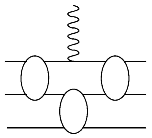
Figure 1: This Feynman diagram represents part a contribution to the seven-point function. The particles are label 1 to 3 from top to bottom. The ovals represent two-body scattering matrices.

Here the virtual photon is absorbed on particle 1 and is preceded by two-body interactions between particles 1 and 2. Between these interactions is two-body t-matrix for particles 2 and 3. Since this is a Feynman diagram, there is no ordering implied between the absorbed photon and the t-matrix for particles 2 and 3. In summing the interactions this t-matrix can either be associated with the sum on the left or with the sum on the right, but not with both. As a result, if we associate this interaction with the right hand sum the last interaction to the right must be between particles two and three while the first interaction on the left must be between particles 1 and 2. This requires that there must be a restricted sum between three-body scattering matrices which occur on either side of a one-body current. The possibility of double-counting this contribution was pointed out in kb97II . The seven-point function can then be written as

$${\cal G}^{\mu} = -\sum_{t=1}^{3}\left(G^{0}_{BS}-G^{0}_{BS}\sum_{i,j=0}^{3}{\cal T}^{ij}B_{jt}G^{0}_{BS}\right)J^{t\mu}\left(G^{0}_{BS}-G^{0}_{BS}\sum_{k,l=0}^{3}{\cal T}^{kl}G^{0}_{BS}\right)$$ (46)

$$-{\cal G}\left(\sum_{t=0}^{3}J^{t\mu}_{\rm ex}\right){\cal G}\,,$$

where the restricted sum is represented by the $B_{jt}$ associated with the left-hand t-matrix. While the exchange current term is nicely factored with complete interacting six-point propagators on the left and right of the current operator, the one-body current term is not factored in this way. This factorization can be accomplished by using the identity

$${\cal G}^{-1}\left(G^{0}_{BS}-G^{0}_{BS}\sum_{i,j=0}^{3}{\cal T}^{ij}B_{jt}G^{0}_{BS}\right)=1+{\cal V}^{t}G^{0}_{BS}=1+V^{t}iG^{t}_{BS}\,,$$ (47)

to rewrite the seven-point propagator (46) as

$${\cal G}^{\mu} = -{\cal G}\left(\sum_{t=1}^{3}\left((1+{\cal V}^{t}G^{0}_{BS})J^{t\mu}+J^{(2)\mu}_{t}G_{t}^{-1}\right)+J^{(3)\mu}\right){\cal G}$$ (48)

$$= -{\cal G}\left[\sum_{t=1}^{3}J^{t\mu}+\sum_{t=0}^{3}J_{\rm int}^{t\mu}\right]{\cal G}\,,$$

where we have defined the one-body and interaction currents in three-particle space $J^{t\mu}$ and $J_{\rm int}^{t\mu}$, respectively, by eq. (42) and by

$$J_{\rm int}^{t\mu} = J^{t\mu}_{ex}+iV^{t}J^{\mu}_{t}\,\quad\mbox{for}\ t\neq 0\,,$$ (49)

$$J_{\rm int}^{0\mu} = J_{\rm ex}^{0\mu}=J^{(3)\mu}\,,$$ (50)

since

$${\cal V}^{t}G^{0}_{BS}J^{t\mu}=iV^{t}J^{\mu}_{t}$$ (51)

behaves like a two-body current.

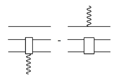
Figure 2: A diagrammatic representation of the interaction current resulting from the symmetric factorization of the seven-point function. The rectangular box represents the two-body Bethe-Salpeter kernel and the rectangular box with attached photon represents the corresponding two-body electromagnetic current.

Thus, the total Bethe-Salpeter current is identified as

$$J^{\mu}_{\rm eff}=\sum_{t=1}^{3}J^{t\mu}+\sum_{t=0}^{3}J^{t\mu}_{\rm int}=J^{(1)\mu}+J^{\mu}_{\rm int}\,,$$ (52)

and the WT identity for this current can be easily shown to be

$$q_{\mu}J^{\mu}_{\rm eff}=\left[e_{T}(q),{\cal G}^{-1}\right]\,.$$ (53)

This along with the wave equation for the bound and scattering states implies that matrix elements of this current between any three-body states is gauge invariant:

$$q_{\mu}{\cal T}^{\mu}=q_{\mu}<\Psi^{\prime}|\,J^{\mu}_{\rm eff}\,|\Psi>=0\,.$$ (54)

III.3 Identical particles

For the case of identical particles it is necessary to explicitly symmetrize the n-point functions. In particular, the transition to the corresponding functions for the Gross equation is simplified by writing the n-point functions in terms of explicitly symmetrized interactions. Any full operator (summed over all three particles) ${\cal R}$ (e.g. ${\cal R}={\cal V},{\cal T},{\cal G},J^{(1)\mu},J^{\mu}_{\rm int},J^{\mu}_{\rm eff},\dots$) commutes with any particle interchange operator ${\cal P}_{ij}$: ${\cal R}={\cal P}_{ij}{\cal R}{\cal P}_{ij}$. Therefore we can write for its symmetrized form $R$

$$R = {\cal A}_{3}{\cal R}={\cal R}{\cal A}_{3}={\cal A}_{3}{\cal R}{\cal A}_{3}\,,$$ (55)

$$R = {\cal A}_{3}R=R{\cal A}_{3}\,,$$ (56)

where the normalized three-body symmetrization operator is

$${\cal A}_{3}\equiv \frac{1}{3!}\left(1+\zeta{\cal P}_{12}+\zeta{\cal P}_{13}+\zeta{\cal P}_{23}+{\cal P}_{4}+{\cal P}_{5}\right)$$

$$= \frac{1}{3!}\left(1+\zeta{\cal P}_{ij}\right)\left(1+\zeta{\cal P}_{ik}+\zeta{\cal P}_{jk}\right)={\cal A}^{k}_{2}\,\Pi_{k}$$

$$= \frac{1}{3!}\left(1+\zeta{\cal P}_{ik}+\zeta{\cal P}_{jk}\right)\left(1+\zeta{\cal P}_{ij}\right)=\Pi_{k}\,{\cal A}^{k}_{2}\,,$$ (57)

with $\zeta=1$ ($\zeta=-1$) for bosons (fermions), respectively, and with

$${\cal P}_{4}= {\cal P}_{13}{\cal P}_{12}={\cal P}_{23}{\cal P}_{13}={\cal P}_{12}{\cal P}_{23}\,,$$

$${\cal P}_{5}= {\cal P}_{23}{\cal P}_{12}={\cal P}_{12}{\cal P}_{13}={\cal P}_{13}{\cal P}_{23}\,,$$ (58)

and with ${\cal A}^{k}_{2}$ being the two body symmetrization operator acting in the two-body subspaces of particles $i$ and $j$ (where $i\neq j\neq k$) and the sum of additional exchanges mixing this subspace with other channel, which we denote $\Pi_{k}$:

$${\cal A}^{k}_{2} = \frac{1}{2}\left(1+\zeta{\cal P}_{ij}\right)\,,$$ (59)

$$\Pi_{k} = \frac{1}{3}\left(1+\zeta{\cal P}_{ki}+\zeta{\cal P}_{kj}\right)\,.$$ (60)

Note that ${\cal A}_{3}={\cal A}_{3}{\cal A}^{k}_{2}={\cal A}^{k}_{2}{\cal A}_{3}$ for any $k$. We will exploit this property in the following discussion.

The symmetrized t-matrix reads

$$T={\cal A}_{3}{\cal T}=V-VG^{0}_{BS}T=V-TG^{0}_{BS}V\,,$$ (61)

with $V$ being the symmetrized potential:

$$V={\cal A}_{3}{\cal V}={\cal A}_{3}V^{0}+\sum_{i=1}^{3}\Pi_{i}\,\overline{V^{i}}iG^{-1}_{i}\,,$$ (62)

where $\overline{V^{i}}={\cal A}^{i}_{2}V^{i}$ is the symmetrized two particle interaction. The symmetrized six-point function can then be written as

$$G={\cal A}_{3}{\cal G}={\cal A}_{3}G^{0}_{BS}-G^{0}_{BS}TG^{0}_{BS}={\cal A}_{3}G^{0}_{BS}-G^{0}_{BS}VG={\cal A}_{3}G^{0}_{BS}-GVG^{0}_{BS}\,.$$ (63)

From eqs. (61,63) the symmetrized bound and scattering state wave functions follow as in previous section. It is easy to see that for full wave functions it holds

$$|\Psi_{s}>={\cal A}_{3}|\Psi>\,.$$ (64)

One can also define the symmetrized Faddeev components of wave functions:

$$|\Psi_{s}^{0}> = {\cal A}_{3}|\Psi^{0}>\,,$$ (65)

$$|\Psi_{s}^{i}> = \frac{1}{3}\left(\,{\cal A}^{i}_{2}|\Psi^{i}>+\zeta{\cal P}_{ij}{\cal A}^{j}_{2}|\Psi^{j}>+\zeta{\cal P}_{ik}{\cal A}^{k}_{2}|\Psi^{k}>\,\right)\,,$$ (66)

where $i\neq j\neq k$. Making use of the symmetry relations (300) the symmetrized wave functions is expressed in terms of only two of these components:

$$|\Psi_{s}>=|\Psi_{s}^{0}>+(1+\zeta{\cal P}_{12}+\zeta{\cal P}_{13})|\Psi_{s}^{1}>=|\Psi_{s}^{0}>+3\Pi_{1}|\Psi_{s}^{1}>\,.$$ (67)

The symmetrized seven-point function can be written as

$$G^{\mu}={\cal A}_{3}{\cal G}^{\mu}=-G\,J^{\mu}_{\rm eff}\,G\,,$$ (68)

and the symmetrized current matrix elements are

$$T^{\mu}=<\Psi_{s}^{\prime}|\,J^{\mu}_{\rm eff}\,|\Psi_{s}> = <\Psi_{s}^{{}^{\prime}0}|\,J^{\mu}_{\rm eff}\,|\Psi_{s}^{0}>+3<\Psi_{s}^{{}^{\prime}0}|\,J^{\mu}_{\rm eff}\,|\Psi_{s}^{1}>+$$ (69)

$$3<\Psi_{s}^{{}^{\prime}1}|\,J^{\mu}_{\rm eff}\,|\Psi_{s}^{0}>+3<\Psi_{s}^{{}^{\prime}1}|\,J^{\mu}_{\rm eff}\,(1+2\zeta{\cal P}_{12})|\Psi_{s}^{1}>\,,$$

where we have used the symmetry relations for the Faddeev components of wave functions and the fact that the current commutes with any replacement operator ${\cal P}_{ij}$.

The BS formalism can be conveniently represented in the matrix notation with matrix indices corresponding to the Faddeev components. This matrix notation is particularly useful for further re-arrangement leading to the spectator formalism. We give a detail description of this matrix notation in appendices.

IV The Three-Body Gross Equation

IV.1 T-matrix and wave functions

The three-body Gross equations can be obtained from the three-body Bethe-Salpeter equations by placing two of the intermediate-state particles on their respective positive energy mass shells. For amplitudes whose first or last interactions are two-body interactions, one of these on-shell particles must be the spectatorGr82 . For amplitudes whose first of last interaction are three-body interactions any pair of on-shell particle can be selectedGr82 . This prescription will work only for three identical particles since it precludes the possibility that the on-shell pair can form a bound state. Since the choice of two of the particles to be set on shell clearly violates the quantum symmetry of the three-body system, it is necessary to symmetrize the interaction kernels to impose the appropriate symmetry of the system, as was done in the case of the two-body system 2Ncur .

The first step in obtaining the three-body Gross equation is to obtain the three-body Bethe-Salpeter equation with symmetrized interactions. This can be done conveniently by first expressing the Faddeev components of the various three-body Bethe-Salpeter amplitudes in terms of four-dimensional matrices and vectors as described in Appendix A. The symmetrization can then also be described in terms of matrices as described in Appendix B. Once the symmetrization is accomplished, it can be noted that the various Faddeev amplitudes can all be expressed in terms of only two types of amplitudes allowing the various amplitudes to be written in terms of two-by-two matrices where the initial (final) interaction is either a three-body interaction, or an interaction between particles 2 and 3. This is the 2-channel formalism of Appendix B. The three-body Gross equation can now be obtained from this two-dimensional matrix form by constraining particles 1 and 2 to the positive-energy mass shell. It can be done conveniently using the operator formalism introduced in 2Ncur .

As described in 2Ncur , a particle can be placed on shell by picking up only the pole of the propagator for this particle when performing energy-loop integrals for the Bethe-Salpeter equation. This can be done by carefully examining these integrals for the various contributions to a given amplitude or by examining all of the Feynman diagrams associated with each amplitude. This can be rather tedious. In 2Ncur , we developed an algebraic approach where various products of operators are defined such that they reproduce the results obtained by choosing poles in the energy integrals. This approach has the additional advantage that, by starting from the corresponding Bethe-Salpeter amplitudes it is possible to obtain expressions for the Gross equation amplitudes that can be easily approximated to any order in various expansion schemes. This was shown in detail for the two-body case in 2Ncur . The primary step in this approach is to replace the propagators for the on-shell nucleons using the identity

$$G_{i}=i{\cal Q}_{i}+\Delta G_{i}\,,$$ (70)

where ${\cal Q}_{i}$ is the operator that places the particle on shell and $\Delta G_{i}$ is the difference between the full propagator and its on-shell contribution. Note that $\Delta G_{i}$ is simply the one-body Feynman propagator with the wrong boundary condition.

Starting with the two-dimensional forms of the Bethe-Salpeter amplitudes, we replace the three-body Feynman propagator with the sum of a piece with particles 1 and 2 on shell $g^{1}_{2}{\cal Q}_{1}{\cal Q}_{2}$ and a remainder $\Delta g^{1}_{2}$ using

$$G^{0}_{BS} = -G_{1}G_{2}G_{3}=-(i{\cal Q}_{1}+\Delta G_{1})(i{\cal Q}_{2}+\Delta G_{2})G_{3}$$ (71)

$$= g^{1}_{2}{\cal Q}_{1}{\cal Q}_{2}+\Delta g^{1}_{2}\,,$$

$$g^{1}_{2} = G_{3}\,,$$ (72)

$$\Delta g^{1}_{2} = \left(-i{\cal Q}_{1}\Delta G_{2}-\Delta G_{1}i{\cal Q}_{2}-\Delta G_{1}\Delta G_{2}\right)G_{3}\,.$$ (73)

Substituting this into the two-dimensional form of the Bethe-Salpeter scattering matrix (360) gives

$$\bm{t}=\bm{v}-\bm{v}\,\bm{\delta}\,(g^{1}_{2}{\cal Q}_{1}{\cal Q}_{2}+\Delta g^{1}_{2})\,\bm{t}\,,$$ (74)

where the matrix $\bm{\delta}$ is defined by (350). This can in turn be reexpressed as a pair of coupled equations as

$$\bm{t} = \bm{u}-\bm{u}g^{1}_{2}{\cal Q}_{1}{\cal Q}_{2}\bm{\delta}\,\bm{t}=\bm{u}-\bm{t}g^{1}_{2}{\cal Q}_{1}{\cal Q}_{2}\bm{\delta}\,\bm{u}\,,$$ (75)

$$\bm{u} = \bm{v}-\bm{v}\,\Delta g^{1}_{2}\bm{\delta}\,\bm{u}=\bm{v}-\bm{u}\,\Delta g^{1}_{2}\bm{\delta}\,\bm{v}\,,$$ (76)

where $\bm{u}$ is the quasipotential.

This system of equations is closed by multiplying from left and right by ${\cal Q}_{1}{\cal Q}_{2}$ which leads to

$$\bm{t}^{1}_{2}=\bm{u}^{1}_{2}-\bm{u}^{1}_{2}\,g^{1}_{2}\,\bm{\delta}\,\bm{t}^{1}_{2}=\bm{u}^{1}_{2}-\bm{t}^{1}_{2}\,g^{1}_{2}\,\bm{\delta}\,\bm{u}^{1}_{2}\,,$$ (77)

where $\bm{u}^{1}_{2}={\cal Q}_{1}{\cal Q}_{2}\bm{u}{\cal Q}_{1}{\cal Q}_{2}$ and $\bm{t}^{1}_{2}={\cal Q}_{1}{\cal Q}_{2}\bm{t}{\cal Q}_{1}{\cal Q}_{2}$.

Although (77) appears to be much like the three-body Beth-Salpeter equation (360), it is in fact much more complicated due to the quasipotential equation (76). The appearance of the matrix $\bm{\delta}$ in (76) means that, in general, the quasipotential matrix is also nondiagonal whereas the Bethe-Salpeter kernel $\bm{v}$ is diagonal. In accordance with (323) we denote

$$\bm{u}=\left(\begin{array}[]{cc}U^{00}&U^{01}\\ U^{10}&U^{11}\end{array}\right)\,.$$ (78)

The off-diagonal components of $\bm{u}$ are the result of mixing contributions from the two- and three-body Bethe-Salpeter kernels which results in contributions which are also completely connected and behave as three-body interactions. The diagonal elements will also be complicated by $\bm{\delta}$. The upper left-hand component $U^{00}$ will always contain at least one contribution from the three-body Bethe-Salpeter kernel in all of its terms, so it will always behave as a three-body interaction even though contributions from the two-body Bethe-Salpeter kernel will also occur.

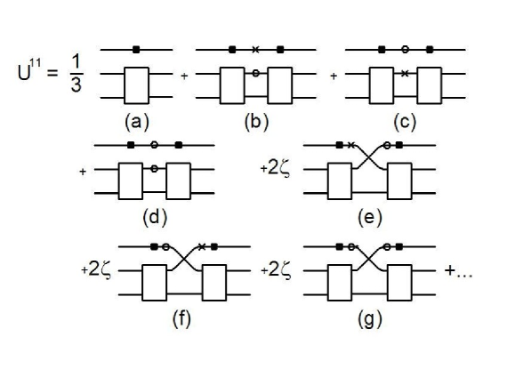
Figure 3: Contributions to $U^{11}$ up to second order in Bethe-Salpeter kernel. The rectangular boxes represent the (symmetrized) two-body Bethe-Salpeter kernel, the crosses represent on-shell propagators, the open circles represent the off-shell propagators and the filled squares represent factors of the inverse one-body propagator.

The lower right-hand contribution $U^{11}$ will also be complicated by this mixing. Figure 3 shows diagrams for $U^{11}$ associated with the first iteration of (76):

$$U^{11}\simeq\frac{1}{3}\overline{V}^{1}iG_{1}^{-1}-\frac{1}{3}\overline{V}^{1}iG_{1}^{-1}\Delta g^{1}_{2}(1+2\zeta{\cal P}_{12})iG_{1}^{-1}\overline{V}^{1}\,.$$ (79)

The rectangular boxes represent the two-body Bethe-Salpeter kernel for particles two and three, the cross represents the on-shell propagator $iQ_{1}$, the open circle represents the off-shell propagator $\Delta G_{i}$ and the square box represents the inverse one-body propagator $iG_{1}^{-1}$. These diagrams therefore contain some ill-defined products such as $Q_{1}G_{1}^{-1}$ that can be resolved only when the quasipotential is used as part of some larger diagram. The resolution of these products is then obtained by using the rules developed in 2Ncur which are repeated in Appendix C for convenience.

Note that in Fig. 3, particle 1 is disconnected from particles 2 and 3 in diagrams (a-d), while the diagrams (e-g) are completely connected. In (77), the quasipotential appears only with the external legs for particles 1 and 2 constrained to be on shell due to (392) and (393). Using these, the completely constrained quasipotential contains only diagrams (a) and (b) which are disconnected and have the form of two-body interactions. As we will see below, the quasipotential with only the initial or final legs constrained can contribute to effective current operator and diagrams (e) and (f) can appear in that role. Diagrams (c), (d) and (g) will never contribute.

Figure 4: Selected diagrams contributing to $U^{11}$ at third order in the Bethe-Salpeter kernels. The large rectangular box represents the three-body Bethe-Salpeter kernel.

There will be many diagrams that contribute to $U^{11}$ at the second iteration of (76). Examples of such diagrams are shown in Fig. 4. Diagram (a) is disconnected and can be categorized as a two-body interaction. Diagrams (b) and (c) are, however, completely connected diagrams and are three-body interactions. Therefore, $U^{11}$ contains both two- and three-body interactions.

As a practical matter, it may be useful to separate the two- and three-body interactions. This can be done by first defining a new, diagonal quasipotential

$$\bm{w}=\bm{v}-\bm{v}\Delta g^{1}_{2}\bm{\alpha}\bm{w}=\bm{v}-\bm{w}\Delta g^{1}_{2}\bm{\alpha}\bm{v}=\left(\begin{array}[]{cc}{\cal A}_{3}W^{0}&0\\ 0&\frac{1}{3}\overline{W}^{1}iG_{1}^{-1}\end{array}\right)\,,$$ (80)

where the diagonal matrix $\bm{\alpha}$ is given by (335). Thus the upper left-hand component of $\bm{w}$ is an iteration of the three-body Bethe-Salpeter kernel, while the lower right hand component is an iteration of the two-body Bethe-Salpeter kernel:

$$\overline{W}^{1}=\overline{V}^{1}-\overline{V}^{1}(-i\Delta G_{2}G_{3})\overline{W}^{1}\,,$$ (81)

i.e., $\overline{W}^{1}$ is the two-body spectator quasipotential for particles 2 and 3.The component $W^{11}=\frac{1}{3}\overline{W}^{1}iG_{1}^{-1}$ is identical to the two-body contribution to $U^{11}$. Indeed, $\bm{u}$ is related to $\bm{w}$ by

$$\bm{u}=\bm{w}-\bm{w}\Delta g^{1}_{2}\bm{\beta}\bm{u}\,,$$ (82)

where the matrix $\bm{\beta}$ is given by (354). The matrix $\bm{w}$ can now be written as the sum of two- and three-body contributions as

$$\bm{w}=\bm{w}^{(2)}+\bm{w}^{(3)}.$$ (83)

Since $\bm{w}^{(2)}$ is identical to the two-body content of $\bm{u}$, $\bm{u}$ can be written as

$$\bm{u}=\bm{w}^{(2)}+\bm{u}^{(3)}.$$ (84)

Substituting (83) and (84) into (82), the equation for the three-body contributions to $\bm{u}$ is

$$\bm{u}^{(3)}=\bm{w}^{(3)}-\bm{w}\Delta g^{1}_{2}\bm{\beta}\bm{w}^{(2)}-\bm{w}\Delta g^{1}_{2}\bm{\beta}\bm{u}^{(3)}\,.$$ (85)

Equation (75) can be resumed to give

$$\bm{t}=\bm{m}-\bm{m}{\cal Q}_{1}{\cal Q}_{2}g^{1}_{2}\,\bm{\beta}\,\bm{t}\,,$$ (86)

where

$$\bm{m}=\bm{u}-\bm{u}{\cal Q}_{1}{\cal Q}_{2}g^{1}_{2}\bm{\alpha}\bm{m}\,.$$ (87)

Since, in general, $\bm{u}$ is not diagonal, $\bm{m}$ is also not diagonal and all of its components contain three-body interactions. It is also useful to separate the two- and three-body contributions to $\bm{m}$. The two-body contribution will just contain iterations of the two-body contribution to $\bm{u}$. We can then define the two-body scattering matrix as

$$\bm{m}^{(2)}=\bm{w}^{(2)}-\bm{w}^{(2)}{\cal Q}_{1}{\cal Q}_{2}g^{1}_{2}\bm{\alpha}\bm{m}^{(2)}\,.$$ (88)

Substituting $\bm{m}=\bm{m}^{(2)}+\bm{m}^{(3)}$ into (87) and using (88) the three-body scattering matrix is given by

$$\bm{m}^{(3)}=\bm{u}^{(3)}-\bm{u}^{(3)}{\cal Q}_{1}{\cal Q}_{2}g^{1}_{2}\bm{\alpha}\bm{m}^{(2)}-\bm{u}{\cal Q}_{1}{\cal Q}_{2}g^{1}_{2}\bm{\alpha}\bm{m}^{(3)}\,.$$ (89)

As in the matrix form of BS equation (cf eqs. (362,363)), in the Gross formalism there are two propagators, a right-hand one

$$\bm{g}^{1}_{2R}=g^{1}_{2}\bm{1}-g^{1}_{2}\bm{t}^{1}_{2}\bm{\delta}g^{1}_{2}=g^{1}_{2}\bm{1}-g^{1}_{2}\bm{u}^{1}_{2}\bm{\delta}\bm{g}^{1}_{2R}$$ (90)

with the inverse

$$({\bm{g}^{1}_{2R}})^{-1}=({g^{1}_{2}})^{-1}\bm{1}+\bm{u}^{1}_{2}\bm{\delta}\,,$$ (91)

and a left-hand one

$$\bm{g}^{1}_{2L}=g^{1}_{2}\bm{1}-g^{1}_{2}\bm{\delta}\bm{t}^{1}_{2}g^{1}_{2}=g^{1}_{2}\bm{1}-\bm{g}^{1}_{2L}\bm{\delta}\bm{u}^{1}_{2}g^{1}_{2}$$ (92)

with the inverse

$$({\bm{g}^{1}_{2L}})^{-1}=({g^{1}_{2}})^{-1}\bm{1}+\bm{\delta}\bm{u}^{1}_{2}\,.$$ (93)

The three-body bound-state vertex function can be obtained using (77) and the analytic form of the t-matrix at the bound-state pole. The vertex function satisfies the equation

$$\left|\bm{\gamma}^{1}_{2}\right>=-\bm{u}^{1}_{2}\bm{\delta}g^{1}_{2}\left|\bm{\gamma}^{1}_{2}\right>=-\bm{m}^{1}_{2}\bm{\beta}g^{1}_{2}\left|\bm{\gamma}^{1}_{2}\right>\,.$$ (94)

From the non-linear form of the t-matrix equation in the Gross formalism

$$\bm{t}^{1}_{2}=\bm{u}^{1}_{2}-\bm{t}^{1}_{2}\bm{\delta}g^{1}_{2}\bm{t}^{1}_{2}-\bm{t}^{1}_{2}g^{1}_{2}\bm{\delta}\bm{u}^{1}_{2}\bm{\delta}g^{1}_{2}\bm{t}^{1}_{2}$$ (95)

we get the normalization condition for vertex function (94)

$$1=\left<\bm{\gamma}^{1}_{2}\right|\left[\frac{\partial g^{1}_{2}}{\partial P^{2}}\bm{\delta}-g^{1}_{2}\bm{\delta}\frac{\partial\bm{u}^{1}_{2}}{\partial P^{2}}\bm{\delta}g^{1}_{2}\right]_{P^{2}=M^{2}}\left|\bm{\gamma}^{1}_{2}\right>\,.$$ (96)

The bound-state Gross wave function is defined as

$$\left|\bm{\psi}^{1}_{2}\right>=g^{1}_{2}\left|\bm{\gamma}^{1}_{2}\right>\,.$$ (97)

Using (94) it is straightforward to show that

$$({\bm{g}^{1}_{2R}})^{-1}\left|\bm{\psi}^{1}_{2}\right>=\left<\bm{\psi}^{1}_{2}\right|({\bm{g}^{1}_{2L}})^{-1}=0\,.$$ (98)

The Gross wave functions for the scattering states can be obtained by considering the analytic properties of $({\bm{g}^{1}_{2L}})^{-1}$, and then the effective current operator can be determined in a similar fashion from the seven-point function (386) and the substitution (71). An alternative approach is to express the Bethe-Salpeter wave functions in terms of the corresponding Gross wave functions. To do this substitute (71) into the Möller operator giving

$$\bm{{1}}-\bm{\delta}\bm{t}{G}^{0}_{BS}=\bm{{1}}-\bm{\delta}\bm{t}\left(g^{1}_{2}{\cal Q}_{1}{\cal Q}_{2}+\Delta g^{1}_{2}\right)=\bm{{1}}-\bm{\delta}\bm{t}g^{1}_{2}{\cal Q}_{1}{\cal Q}_{2}-\bm{\delta}\bm{t}\Delta g^{1}_{2}\,.$$ (99)

Using (75) to replace the t-matrix in the last term gives

$$\bm{{1}}-\bm{\delta}\bm{t}{G}^{0}_{BS} = \bm{{1}}-\bm{\delta}\bm{t}g^{1}_{2}{\cal Q}_{1}{\cal Q}_{2}-\bm{\delta}\left(\bm{u}-\bm{t}g^{1}_{2}{\cal Q}_{1}{\cal Q}_{2}\bm{\delta}\bm{u}\right)\Delta g^{1}_{2}$$ (100)

$$= \left(\bm{1}-\bm{\delta}\bm{t}g^{1}_{2}{\cal Q}_{1}{\cal Q}_{2}\right)\left(\bm{1}-\bm{\delta}\bm{u}\Delta g^{1}_{2}\right)\,.$$

Similarly, the right-hand Möller operator can be rewritten as

$$\bm{{1}}-{G}^{0}_{BS}\bm{t}\bm{\delta}=\left(\bm{1}-\Delta g^{1}_{2}\bm{u}\bm{\delta}\right)\left(\bm{1}-g^{1}_{2}{\cal Q}_{1}{\cal Q}_{2}\bm{t}\bm{\delta}\right)\,.$$ (101)

By examining the bound-state pole in the t-matrices, we can find expressions for the Bethe-Salpeter bound-state wave functions in term of the corresponding Gross wave functions:

$$\left<\bm{\psi}\right|=\left<\bm{\psi}^{1}_{2}\right|\left(\bm{1}-\bm{\delta}\bm{u}\Delta g^{1}_{2}\right)$$ (102)

and

$$\left|\bm{\psi}\right>=\left(\bm{1}-\Delta g^{1}_{2}\bm{u}\bm{\delta}\right)\left|\bm{\psi}^{1}_{2}\right>\,.$$ (103)

The three-body scattering final state can be obtained directly from the two-dimensional form of the corresponding Bethe-Salpeter state (371) as

$$\left<\bm{{\psi}}^{(-)}\right| = \frac{1}{4}\left<\bm{p}_{1},s_{1};\bm{p}_{2},s_{2};\bm{p}_{3},s_{3}\right|{\cal A}_{3}\bm{{d}}^{T}\left[\bm{{1}}-\bm{\delta}\bm{t}G^{0}_{BS}\right]$$ (104)

$$= \frac{1}{4}\left<\bm{p}_{1},s_{1};\bm{p}_{2},s_{2};\bm{p}_{3},s_{3}\right|{\cal A}_{3}\bm{{d}}^{T}\left(\bm{1}-\bm{\delta}\bm{t}g^{1}_{2}{\cal Q}_{1}{\cal Q}_{2}\right)\left(\bm{1}-\bm{\delta}\bm{u}\Delta g^{1}_{2}\right)$$

$$= \left<\bm{{\psi}}^{1(-)}_{2}\right|\left(\bm{1}-\bm{\delta}\bm{u}\Delta g^{1}_{2}\right)$$

where

$$\left<\bm{{\psi}}^{1(-)}_{2}\right|=\frac{1}{4}\left<\bm{p}_{1},s_{1};\bm{p}_{2},s_{2};\bm{p}_{3},s_{3}\right|{\cal A}_{3}\bm{{d}}^{T}\left[\bm{{1}}-\bm{\delta}\bm{t}^{1}_{2}g^{1}_{2}\right]$$ (105)

is the Gross three-body scattering state which satisfies the wave equation

$$\left<\bm{{\psi}}^{1(-)}_{2}\right|({\bm{g}^{1}_{2L}})^{-1}=0\,.$$ (106)

Finding a similar relation for the two-body final scattering state is a little more complicated since it contains a two-body bound state which also needs to be re-expressed in terms of the corresponding spectator wave function for two-body bound state as well as rewriting a Möller operator of a slightly different form than that examined above. The two-body final state in the two-dimensional matrix form is given by (380)

$$\left<\bm{\phi}^{1(-)}\right|=\frac{1}{3}\left<\Phi^{(2)1};\bm{p}_{1},s_{1}\right|{\cal A}_{23}\left(\begin{array}[]{cc}0&1\end{array}\right)\left(\bm{1}-\bm{\beta}\bm{t}\bm{G}^{0}_{BS}\right)\,.$$ (107)

The symmetrized two-body spectator bound-state wave function is for particles 2 and 3 is defined as

$$\left|\varphi^{(2)}_{2}\right>={\cal Q}_{2}{\cal A}_{23}\left|\Phi^{(2)}\right>\,.$$ (108)

and satisfies the equation

$$(G_{3}^{-1}+\overline{W}^{11}_{22})\left|\varphi^{(2)}_{2}\right>=0\,,$$ (109)

where $\overline{W}^{11}_{22}={\cal Q}_{2}\overline{W}^{1}{\cal Q}_{1}{\cal Q}_{2}$. The corresponding Bethe-Salpeter wave function can be expressed in terms of the spectator wave function one by

$${\cal A}_{23}\left|\Phi^{(2)}\right>=\left[1-(-i\Delta G_{2}G_{3})\overline{W}^{1}\right]\left|\varphi^{(2)}_{2}\right>\,.$$ (110)

The asymptotic spectator state satisfies the equation

$$\left<\varphi^{(2)}_{2};\bm{p}_{1},s_{1}\right|\left[G_{3}^{-1}+\overline{W}^{11}_{22}\right]=0\,,$$ (111)

and the asymptotic state in (107) can be now written in terms of this spectator state as

$$\left<\Phi^{(2)1};\bm{p}_{1},s_{1}\right|{\cal A}_{23}=\left<\varphi^{(2)}_{2};\bm{p}_{1},s_{1}\right|{\cal Q}_{1}\left[1-\overline{W}^{1}\left(-i{\cal Q}_{1}\Delta G_{2}G_{3}\right)\right]\,.$$ (112)

From ${\cal Q}_{1}\Delta g^{1}_{2}=-i{\cal Q}_{1}\Delta G_{2}G_{3}$, it follows

$${\cal Q}_{1}\,\left[1-\overline{W}^{1}\left(-i{\cal Q}_{1}\Delta G_{2}G_{3}\right)\right]\left(\begin{array}[]{cc}0&1\end{array}\right)={\cal Q}_{1}\,\left(\begin{array}[]{cc}0&1\end{array}\right)\left(\bm{1}-\bm{\alpha}\bm{w}\Delta g^{1}_{2}\right)\,.$$ (113)

The Bethe-Salpeter scattering state can now be written as

$$\left<\bm{\phi}^{1(-)}\right| = \frac{1}{3}\left<\varphi^{(2)}_{2};\bm{p}_{1},s_{1}\right|\left(\begin{array}[]{cc}0&1\end{array}\right)\left(\bm{1}-\bm{\alpha}\bm{w}\Delta g^{1}_{2}\right)\left(\bm{1}-\bm{\beta}\bm{t}\bm{G}^{0}_{BS}\right)$$ (115)

Using the identity

$$\left(\bm{1}-\bm{\alpha}\bm{w}\Delta g^{1}_{2}\right)\left(\bm{1}-\bm{\beta}\bm{t}\bm{G}^{0}_{BS}\right)=\left[\bm{1}-\left(\bm{1}-\bm{\alpha}\bm{w}\Delta g^{1}_{2}\right)\bm{\beta}\bm{t}{\cal Q}_{1}{\cal Q}_{2}g^{1}_{2}\right]\left(\bm{1}-\bm{\delta}\bm{u}\Delta g^{1}_{2}\right)\,,$$ (116)

this can be rewritten as

$$\left<\bm{\phi}^{1(-)}\right| = \frac{1}{3}\left<\varphi^{(2)}_{2};\bm{p}_{1},s_{1}\right|\left(\begin{array}[]{cc}0&1\end{array}\right)\left[\bm{1}-\left(\bm{1}-\bm{\alpha}\bm{w}\Delta g^{1}_{2}\right)\bm{\beta}\bm{t}{\cal Q}_{1}{\cal Q}_{2}g^{1}_{2}\right]\left(\bm{1}-\bm{\delta}\bm{u}\Delta g^{1}_{2}\right)$$ (118)

$$= \left<\bm{\phi}^{1(-)}_{2}\right|\left(\bm{1}-\bm{\delta}\bm{u}\Delta g^{1}_{2}\right)\,,$$ (119)

where

$$\left<\bm{\phi}^{1(-)}_{2}\right|=\frac{1}{3}\left<\varphi^{(2)}_{2};\bm{p}_{1},s_{1}\right|\left(\begin{array}[]{cc}0&1\end{array}\right)\left[\bm{1}-\left(\bm{1}-\bm{\alpha}\bm{w}\Delta g^{1}_{2}\right)\bm{\beta}\bm{t}{\cal Q}_{1}{\cal Q}_{2}g^{1}_{2}\right]$$ (120)

is the Gross two-body scattering state. It satisfies the equation

$$\left<\bm{\phi}^{1(-)}_{2}\right|({\bm{g}^{1}_{2L}})^{-1}=0\,.$$ (121)

IV.2 Electromagnetic current

According to previous subsection, the relationship of the Bethe-Salpeter to Gross wave functions always involves a factor of $\left(\bm{1}-\Delta g^{1}_{2}\bm{u}\bm{\delta}\right)$ for initial states and $\left(\bm{1}-\bm{\delta}\bm{u}\Delta g^{1}_{2}\right)$ for final states. Any Bethe-Salpeter current matrix element can now be converted to the corresponding Gross matrix element by defining the effective current for the Gross equation as

$$\bm{j}^{1\mu}_{2\,{\rm eff}}={\cal Q}_{1}{\cal Q}_{2}\left(\bm{1}-\bm{\delta}\bm{u}\Delta g^{1}_{2}\right)\bm{j}^{\mu}_{\rm eff}\left(\bm{1}-\Delta g^{1}_{2}\bm{u}\bm{\delta}\right){\cal Q}_{1}{\cal Q}_{2}\,,$$ (122)

where $\bm{j}^{\mu}_{\rm eff}$ is given by (387) and (388).

Contraction of the photon four-momentum with this effective current operator yields

$$q_{\mu}\bm{j}^{1\mu}_{2\,{\rm eff}} = {\cal Q}_{1}{\cal Q}_{2}\left(\bm{1}-\bm{\delta}\bm{u}\Delta g^{1}_{2}\right)\left(e_{T}(q)\bm{\delta}\bm{g}_{R}^{-1}-\bm{g}_{L}^{-1}e_{T}(q)\bm{\delta}\right)\left(\bm{1}-\Delta g^{1}_{2}\bm{u}\bm{\delta}\right){\cal Q}_{1}{\cal Q}_{2}$$ (123)

$$= {\cal Q}_{1}{\cal Q}_{2}\left[e_{3}(q)\bm{\delta}\left(G_{3}^{-1}\bm{1}+\bm{u}\bm{\delta}\right)-\left(G_{3}^{-1}\bm{1}+\bm{\delta}\bm{u}\right)e_{3}(q)\bm{\delta}\right]{\cal Q}_{1}{\cal Q}_{2}$$

$$= e_{3}(q)\bm{\delta}{\cal Q}_{1}{\cal Q}_{2}({\bm{g}^{1}_{2R}})^{-1}-({\bm{g}^{1}_{2L}})^{-1}{\cal Q}_{1}{\cal Q}_{2}\bm{\delta}e_{3}(q)\,,$$

where the rules of Appendix C have been used to simplify this expression (the proof is similar to that for a two-body system described in detail in Sec. 3.2 of ref. 2Ncur ). This, along with the wave equations for the Gross wave functions, implies that the current is conserved.

To bring the expression for the effective current to a form that can be more readily used for practical calculation requires use of the non-associative algebra for the on-shell operators ${\cal Q}_{i}$ and the propagators developed in 2Ncur and summarized in Appendix C. The pieces of primary concern are those involving the one-body current and can be simplified with the following identities:

$${\cal Q}_{1}{\cal Q}_{2}J^{(1)\mu}{\cal Q}_{1}{\cal Q}_{2}={\cal Q}_{1}{\cal Q}_{2}J^{\mu}_{3}\,,$$ (124)

$${\cal Q}_{1}{\cal Q}_{2}J^{(1)\mu}\Delta g^{1}_{2}={\cal Q}_{1}{\cal Q}_{2}\left(J^{\mu}_{1}G_{1}+J^{\mu}_{2}G_{2}\right)\,,$$ (125)

$$\Delta g^{1}_{2}J^{(1)\mu}{\cal Q}_{1}{\cal Q}_{2}=\left(G_{1}J^{\mu}_{1}+G_{2}J^{\mu}_{2}\right){\cal Q}_{1}{\cal Q}_{2}$$ (126)

and

$$\Delta g^{1}_{2}J^{(1)\mu}\Delta g^{1}_{2} = -\left(i{\cal Q}_{1}J^{\mu}_{1}G_{1}+G_{1}J^{\mu}_{1}i{\cal Q}_{1}\right)\Delta G_{2}G_{3}-(\Delta G_{1}J^{\mu}_{1}\Delta G_{1})G_{2}G_{3}$$ (127)

$$-\Delta G_{1}\left(i{\cal Q}_{2}J^{\mu}_{2}G_{2}+G_{2}J^{\mu}_{2}i{\cal Q}_{2}\right)G_{3}-G_{1}(\Delta G_{2}J^{\mu}_{2}\Delta G_{2})G_{3}$$

$$+\left(-i{\cal Q}_{1}\Delta G_{2}-\Delta G_{1}i{\cal Q}_{2}-\Delta G_{1}\Delta G_{2}\right)(G_{3}J^{\mu}_{3}G_{3})\,.$$

In these expressions we have used the identity ${\cal Q}_{i}J_{i}{\cal Q}_{i}=0$ (397) to give ${\cal Q}_{i}J_{i}\Delta G_{i}={\cal Q}_{i}J_{i}G_{i}$ and $\Delta G_{i}J_{i}{\cal Q}_{i}=G_{i}J_{i}{\cal Q}_{i}$. The corresponding part of the effective spectator current then reads:

$$\bm{j}^{1\mu}_{2\,{\rm eff,IA}} = {\cal Q}_{1}{\cal Q}_{2}\,\left[J^{\mu}_{3}\bm{\delta}-\bm{\delta}\bm{u}(G_{1}J^{\mu}_{1}+G_{2}J^{\mu}_{2})\bm{\delta}-\bm{\delta}(J^{\mu}_{1}G_{1}+J^{\mu}_{2}G_{2})\bm{u}\bm{\delta}\right.$$ (128)

$$\left.+\bm{\delta}\bm{u}(\Delta g^{1}_{2}J^{(1)\mu}\Delta g^{1}_{2})\bm{\delta}\bm{u}\bm{\delta}\right]\,{\cal Q}_{1}{\cal Q}_{2}\,,$$

where $\Delta g^{1}_{2}J^{(1)\mu}\Delta g^{1}_{2}$ from the last term is given by eq. (127).

The interaction current also contains a piece containing the one-body current operator that resulted from our symmetric separation of the seven-point function into a current operator and six-point propagators:

$$\bm{j}^{\mu}_{sym}=\frac{1}{3}\left(\begin{array}[]{c}0\\ 1\end{array}\right)i\overline{V}^{1}J^{\mu}_{1}\left(\begin{array}[]{cc}0&1\end{array}\right)\,.$$ (129)

Contributions from this current can be simplified using the identities:

$$Q_{1}Q_{2}i\overline{V}^{1}J^{\mu}_{1}Q_{1}Q_{2}=0\,,$$ (130)

$$Q_{1}Q_{2}i\overline{V}^{1}J^{\mu}_{1}\Delta g^{1}_{2}=-(Q_{1}J^{\mu}_{1}G_{1})(Q_{2}i\overline{V}^{1}G_{2}G_{3})\,,$$ (131)

$$\Delta g^{1}_{2}i\overline{V}^{1}J^{\mu}_{1}Q_{1}Q_{2}=-(G_{1}J^{\mu}_{1}Q_{1})(G_{2}G_{3}i\overline{V}^{1}Q_{2})\,,$$ (132)

and

$$\Delta g^{1}_{2}i\overline{V}^{1}J^{\mu}_{1}\Delta g^{1}_{2} = (iQ_{1}J^{\mu}_{1}G_{1})(\Delta G_{2}G_{3}i\overline{V}^{1}G_{2}G_{3})+(G_{1}J^{\mu}_{1}iQ_{1})(G_{2}G_{3}i\overline{V}^{1}\Delta G_{2}G_{3})$$ (133)

$$+(\Delta G_{1}J^{\mu}_{1}\Delta G_{1})(G_{2}G_{3}i\overline{V}^{1}G_{2}G_{3})\,.$$

The corresponding effective spectator current is given by:

$$\bm{j}^{1\mu}_{2\,{\rm eff,sym}} = {\cal Q}_{1}{\cal Q}_{2}\,\frac{1}{3}\,\bm{\delta}\,\left[\bm{u}\bm{\delta}\left(\begin{array}[]{cc}0&0\\ 0&G_{1}J^{\mu}_{1}i\overline{V}^{1}G_{2}G_{3}\end{array}\right)+\left(\begin{array}[]{cc}0&0\\ 0&J^{\mu}_{1}G_{1}i\overline{V}^{1}G_{2}G_{3}\end{array}\right)\bm{\delta}\bm{u}\right.$$ (141)

$$\left.+\bm{u}\bm{\delta}\left(\begin{array}[]{cc}0&0\\ 0&\Delta g^{1}_{2}i\overline{V}^{1}J^{\mu}_{1}\Delta g^{1}_{2}\end{array}\right)\bm{\delta}\bm{u}\right]\,\bm{\delta}\,{\cal Q}_{1}{\cal Q}_{2}\,.$$

The two-body exchange current part of the interaction current is

$$\bm{j}^{(2)\mu}=\frac{1}{3}\left(\begin{array}[]{c}0\\ 1\end{array}\right)\overline{J}^{1\mu}_{ex}\left(\begin{array}[]{cc}0&1\end{array}\right)\,,$$ (142)

where $\overline{J}^{1\mu}_{ex}=iG_{1}^{-1}\overline{J}^{(2)\mu}_{23}$. Contributions from this current can be simplified using the identities

$$Q_{1}Q_{2}\,\overline{J}^{1\mu}_{ex}\,Q_{1}Q_{2}=Q_{1}Q_{2}\overline{J}^{(2)\mu}_{23}Q_{2}\,,$$ (143)

$$Q_{1}Q_{2}\,\overline{J}^{1\mu}_{ex}\Delta g^{1}_{2}=-iQ_{1}Q_{2}\overline{J}^{(2)\mu}_{23}\Delta G_{2}G_{3}\,,$$ (144)

$$\Delta g^{1}_{2}\,\overline{J}^{1\mu}_{ex}\,Q_{1}Q_{2}=-iQ_{1}\Delta G_{2}G_{3}\overline{J}^{(2)\mu}_{23}Q_{2}$$ (145)

and

$$\Delta g^{1}_{2}\,\overline{J}^{1\mu}_{ex}\,\Delta g^{1}_{2}=-Q_{1}\Delta G_{2}G_{3}\overline{J}^{(2)\mu}_{23}\Delta G_{2}G_{3}+i\Delta G_{1}G_{2}G_{3}\overline{J}^{(2)\mu}_{23}G_{2}G_{3}\,.$$ (146)

The spectator two-body exchange current is thus

$$\bm{j}^{1\mu}_{2\,{\rm eff,ex2}} = {\cal Q}_{1}{\cal Q}_{2}\,\frac{1}{3}\,\bm{\delta}\,\left[\left(\begin{array}[]{cc}0&0\\ 0&\overline{J}^{(2)\mu}_{23}\end{array}\right)+\bm{u}\bm{\delta}\left(\begin{array}[]{cc}0&0\\ 0&\Delta G_{2}G_{3}i\overline{J}^{(2)\mu}_{23}\end{array}\right)+\left(\begin{array}[]{cc}0&0\\ 0&i\overline{J}^{(2)\mu}_{23}\Delta G_{2}G_{3}\end{array}\right)\bm{\delta}\bm{u}\right.$$ (156)

$$\left.+\bm{u}\bm{\delta}\left(\begin{array}[]{cc}0&0\\ 0&\Delta g^{1}_{2}\overline{J}^{1\mu}_{ex}\Delta g^{1}_{2}\end{array}\right)\bm{\delta}\bm{u}\right]\,\bm{\delta}\,{\cal Q}_{1}{\cal Q}_{2}\,.$$

Since the Bethe-Salpeter three-body current is completely connected there is no simplification to the contributions from this current:

$$\bm{j}^{1\mu}_{2\,{\rm eff,ex3}}={\cal Q}_{1}{\cal Q}_{2}\left(\bm{1}-\bm{\delta}\bm{u}\Delta g^{1}_{2}\right)\,\bm{\delta}\,\left(\begin{array}[]{cc}\overline{J}^{0\mu}_{ex}&0\\ 0&0\end{array}\right)\bm{\delta}\,\left(\bm{1}-\Delta g^{1}_{2}\bm{u}\bm{\delta}\right){\cal Q}_{1}{\cal Q}_{2}\,,$$ (157)

The full effective spectator current is the sum of these four contributions (128,141,156,157):

$$\bm{j}^{1\mu}_{2\,{\rm eff}}=\bm{j}^{1\mu}_{2\,{\rm eff,IA}}+\bm{j}^{1\mu}_{2\,{\rm eff,sym}}+\bm{j}^{1\mu}_{2\,{\rm eff,ex2}}+\bm{j}^{1\mu}_{2\,{\rm eff,ex3}}\,.$$ (158)

Clearly, this effective current is quite complicated in its complete form and would correspond to a large number of Feynman diagrams. For the purpose of comparing these result to those of kb97 and Gr04 it is useful to compare the simplest case where the interaction is given by a one-boson-exchange kernel and no three-body contributions are present.

V Spectator formalism in the one-boson-exchange approximation

The expressions presented above for the spectator formalism are exact. However, in any practical calculation using either the Bethe-Salpeter or spectator approaches it is necessary to approximate the equations by truncating the kernels. This is usually done by expanding the kernels in the number of meson exchanges. Indeed, the only solutions that have been obtained for the three-body spectator equations at this time are in the one-boson-exchange approximation. Care must be taken in truncating the kernel in order to maintain the wave equations and Ward identities. In this section, we will simplify the general expressions to the case of the one-boson-exchange (OBE) approximation.

In the OBE approximation the quasipotentials $\bm{u}$ and $\bm{w}$ are equal to Bethe-Salpeter kernel $\bm{v}$ and there are no three-body forces or currents. Then the two-channel formalism developed above reduces to just one independent channel: there is only one independent component of the t-matrix, of the effective current and of the wave functions.

The general expressions for the wave functions and currents given in the previous section can be reduced to this approximation by replacing $\bm{u}$ and $\bm{w}$ by

$$\bm{v}=\left(\begin{array}[]{cc}0&0\\ 0&\frac{1}{3}\overline{V}^{1}iG^{-1}_{1}\end{array}\right)\,.$$ (159)

This implies that the spectator t-matrix becomes

$$\bm{t}^{1}_{2}=\left(\begin{array}[]{cc}0&0\\ 0&T^{11}_{22}\end{array}\right)\,,$$ (160)

where, using (77) with the shorthand notation ${\cal P}=1+2\zeta{\cal P}_{12}$ and $\overline{V}^{11}_{22}={\cal Q}_{1}{\cal Q}_{2}\overline{V}^{1}{\cal Q}_{1}{\cal Q}_{2}$, the nonzero component of $\bm{t}$ is given by Gr82

$$T^{11}_{22}=\frac{1}{3}\overline{V}^{11}_{22}-\overline{V}^{11}_{22}\,G_{3}\,{\cal P}\,T^{11}_{22}=\frac{1}{3}\overline{V}^{11}_{22}-T^{11}_{22}\,G_{3}\,{\cal P}\,\overline{V}^{11}_{22}\,.$$ (161)

The propagators (90) and (92), and their inverses (91) and (93) in the subspace of this symmetrized Faddeev component read:

$$g^{1}_{2R}=G_{3}-3G_{3}\,T^{11}_{22}\,{\cal P}\,G_{3}\,, (g^{1}_{2R})^{-1}=G_{3}^{-1}+\overline{V}^{11}_{22}\,{\cal P}\,,$$ (162)

$$g^{1}_{2L}=G_{3}-3G_{3}{\cal P}\,T^{11}_{22}\,G_{3}\,, (g^{1}_{2L})^{-1}=G_{3}^{-1}+{\cal P}\,\overline{V}^{11}_{22}\,.$$ (163)

The effective current, defined by (128,141,156,157,158), can be simplified by setting the three-body Bethe-Salpeter current to zero, and keeping only terms involving a single boson exchange. This means that in (128), only terms up to first order in $\bm{u}=\bm{v}$ can be retained. In (141) and (156), no terms containing $\bm{u}$ can be retained since the corresponding Bethe-Salpeter currents already contain OBE contributions. Since the three-body current is set to zero, $\bm{j}^{1\mu}_{2\,{\rm eff,ex3}}=0$. Using the rules from Appendix C, the effective current in the OBE approximation is then (still in the two-channel notation):

$$\bm{j}^{1\mu}_{2\,{\rm eff}}={\cal Q}_{1}{\cal Q}_{2}\left[J^{\mu}_{3}\bm{\delta}-\bm{\delta}\left(\begin{array}[]{cc}0&0\\ 0&\frac{1}{3}\left(\overline{V}^{1}G_{2}J^{\mu}_{2}+J^{\mu}_{2}G_{2}\overline{V}^{1}-\overline{J}^{(2)}_{23}\right)\end{array}\right)\bm{\delta}\right]{\cal Q}_{1}{\cal Q}_{2}\,.$$ (164)

To reduce it further to the effective operator in the one-channel space of the OBE approximation, we have to specify first the corresponding wave functions.

Since the three-body contributions have been eliminated, the bound-state wave function (98) has only one nonzero component,

$$\left|\bm{\psi}^{1}_{2}\right>\cong\left(\begin{array}[]{c}0\\ \left|\psi^{1}_{2}\right>\end{array}\right)$$ (165)

where

$$(g^{1}_{2R})^{-1}\,\left|\psi^{1}_{2}\right>=0\,.$$ (166)

This wave equation is represented diagrammatically by Fig. 5a.

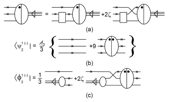
Figure 5: Feynman diagrams representing (a) the bound-state wave equation, (b) the three-body final-state wave function and (c) the two-body final-state wave function in the one-boson exchange approximation.

The interaction-dependent part of the wave function (105) with the t-matrix (160) already has only one component, but the free propagation of three particles is partially included in the 0^th channel, omitted now in the OBE approximation. Notice that the current (164) always acts on the wave functions both from the left-hand and right-hand side with the matrix $\bm{\delta}$. This actually holds for any properly symmetrized one- and two-body operator, the matrix $\bm{\delta}$ just counts all symmetrization factors. Under the action of $\bm{\delta}$ the three-body scattering wave function in the OBE approximation can be replaced by its one component form

$$\bm{\delta}\,\left|\bm{{\psi}}^{1(-)}_{2}\right> = \bm{\delta}\,\frac{1}{4}\left(\bm{{1}}-g^{1}_{2}\bm{t}^{1}_{2}\bm{\delta}\right)\,\bm{d}{\cal A}_{3}\left|\bm{p}_{1},s_{1};\bm{p}_{2},s_{2};\bm{p}_{3},s_{3}\right>$$ (171)

$$\rightarrow \left(\begin{array}[]{c}1\\ {\cal P}\end{array}\right){\cal A}_{3}\,(1-9G_{3}T^{11}_{22})\,\left|\bm{p}_{1},s_{1};\bm{p}_{2},s_{2};\bm{p}_{3},s_{3}\right>=\bm{\delta}\,\left(\begin{array}[]{c}0\\ \left|\psi^{1(-)}_{2}\right>\end{array}\right)\,,$$

$$\left|\psi^{1(-)}_{2}\right> = \frac{1}{3}\left(1-9G_{3}T^{11}_{22}\right){\cal A}_{3}\,\left|\bm{p}_{1},s_{1};\bm{p}_{2},s_{2};\bm{p}_{3},s_{3}\right>\,.$$ (172)

which follows from identities ${\cal A}_{3}{\cal P}=3{\cal A}_{3}$ and

$$\frac{1}{4}\bm{\delta}\,\bm{d}\,{\cal A}_{3} = {\cal A}_{3}\left(\begin{array}[]{c}1\\ {\cal P}\end{array}\right)=\bm{\delta}\,\left(\begin{array}[]{c}0\\ \frac{1}{3}{\cal A}_{3}\end{array}\right)\,,$$ (177)

$$\bm{\delta}\,\left(\begin{array}[]{c}0\\ \left|\psi\right>\end{array}\right) = 3\left(\begin{array}[]{c}1\\ {\cal P}\end{array}\right)\,\left|\psi\right>\,.$$ (182)

Also the three-body scattering wave function in the final state multiplied by the matrix $\bm{\delta}$ is just

$$\left<\bm{{\psi}}^{1(-)}_{2}\right|\,\bm{\delta}=\left(0,\left<\psi^{1(-)}_{2}\right|\,\right)\,\bm{\delta}\,.$$ (183)

Thus in the considered OBE approximation the matrix elements of the current (164) should be evaluated with the one-component scattering wave functions (172). This wave function is diagrammatically represented by Fig. 5b. From the relations (161,163) the proper wave equation

$$\left<\psi^{1(-)}_{2}\right|\,(g^{1}_{2L})^{-1}=0$$ (184)

follows, which indicates that the one-component expression (172) is the correct three-body scattering wave function in the OBE approximation (i.e., not just effectively in the matrix elements of operators proportional to symmetrizing matrix $\bm{\delta}$). This can indeed be verified by repeating the whole construction of this paper for the theory without the explicit three-body force.

Some care must be used in truncating the final two-body scattering state (120). The factor $\bm{1}-\bm{\alpha}\bm{w}\Delta g^{1}_{2}$ must also be expanded in order for this wave function to satisfy the wave equation in the OBE approximation. In this the factor $\bm{w}$ must be expanded to one order less than the order of expansion. Since we are keeping only OBE terms, $\bm{w}$ should contain zero boson exchanges which means that it should be set to zero. This state then also simplifies to the one-component form

$$\left<\bm{\phi}^{1(-)}_{2}\right| = \left(0,\,\left<\phi^{1(-)}_{2}\right|\,\right)\,,$$ (185)

$$\left<\phi^{1(-)}_{2}\right| = \frac{1}{3}\left<\varphi^{2}_{Bs};\bm{p}_{1},s_{1}\right|{\cal Q}_{1}{\cal Q}_{2}\left[1-6\zeta{\cal P}_{12}T^{11}_{22}G_{3}\right]\,,$$ (186)

$$\left<\phi^{1(-)}_{2}\right|\,(g^{1}_{2L})^{-1} = 0\,.$$ (187)

This wave function is represented diagrammatically by Fig. 5c.

Since all wave function have in the OBE approximation only one non-zero component, the matrix element of the effective current (164) can be with the help of (182) rewritten as a matrix element of the effective one-component current $\left(J^{\mu}_{\rm eff}\right)^{11}_{22}$

$$\left<\bm{\psi^{\prime}}\right|\,\bm{j}^{1\mu}_{2\,{\rm eff}}\,\left|\bm{\psi^{\prime}}\right> = \left<\psi^{\prime}\right|\,\left(J^{\mu}_{\rm eff}\right)^{11}_{22}\,\left|\psi\right>\,,$$ (188)

$$\left(J^{\mu}_{\rm eff}\right)^{11}_{22} = {\cal Q}_{1}{\cal Q}_{2}\,3\,\left[\,J^{\mu}_{3}{\cal P}-{\cal P}\left(\overline{V}^{1}G_{2}J^{\mu}_{2}+J^{\mu}_{2}G_{2}\overline{V}^{1}-\overline{J}^{(2)}_{23}\right){\cal P}\,\right]{\cal Q}_{1}{\cal Q}_{2}\,,$$ (189)

where $\psi$ and $\psi^{\prime}$ are any of the wave functions discussed above. The Ward identity for this current is

$$q_{\mu}\left(J^{\mu}_{\rm eff}\right)^{11}_{22} = 3\left\{\left[e_{3}(q),G_{3}^{-1}\right]{\cal Q}_{1}{\cal Q}_{2}{\cal P}-{\cal P}{\cal Q}_{1}{\cal Q}_{2}\left(\left[e_{2}(q),\overline{V}^{1}\right]-\left[e_{2}(q)+e_{3}(q),\overline{V}^{1}\right]\right){\cal Q}_{1}{\cal Q}_{2}{\cal P}\right\}$$ (190)

$$= 3\left\{\left[e_{3}(q),G_{3}^{-1}\right]{\cal Q}_{1}{\cal Q}_{2}{\cal P}+{\cal P}\left[e_{3}(q),\overline{V}^{11}_{22}\right]{\cal P}\right\}$$

$$= 3\left\{{\cal Q}_{1}{\cal Q}_{2}{\cal P}e_{3}(q)(g^{1}_{2R})^{-1}-(g^{1}_{2L})^{-1}e_{3}(q){\cal Q}_{1}{\cal Q}_{2}{\cal P}\right\}\,.$$ (191)

This, along with the wave equations, shows that the current matrix elements will be gauge invariant.

Figure 6 provides a diagrammatic representation of all of the contributions to the one-boson-exchange Gross current.

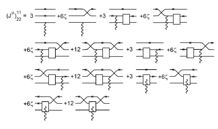
Figure 6: Feynman diagrams representing the effective current operator for the spectator equation in the one-boson-exchange approximation.

The matrix elements for various processes can now be produced by combining the spectator wave functions with this effective current. Some simplification can be obtained by defining off-shell wave functions and scattering matrices. Doing this leads to expressions coinciding with the results of kb97 and Gr04 .

VI Summary

In this paper, we have produced a comprehensive and general description of the three-body spectator equations and the corresponding electromagnetic currents starting with the three-body Bethe-Salpeter equations and using an operator formalism that has been developed for this purpose. Wave functions for bound state, and two- and three-body states are presented along with the effective electromagnetic current operator. The results obtained are exact and can be truncated for practical calculation. As an example we have shown truncation according to the one-boson-exchange approximation is consistent with previous results.

Appendix A Matrix form of the BS equation: Distinguishable Particles

A.1 Propagators and wave functions

To make the equation for t-matrix, one can rewrite them by defining the matrix components

$${\cal V}^{ij} = V^{i}iG^{-1}_{i}\delta_{ij}={\cal V}^{i}\delta_{ij}\,,\qquad i,j=1,2,3$$ (192)

$${\cal V}^{i0} = {\cal V}^{0i}=V^{0}\delta_{i0}={\cal V}^{0}\delta_{i0}\,,$$ (193)

and the same for matrices ${\cal M}$. In terms of these, the equations for the three-body t-matrix reads

$${\cal T}^{ij}={\cal V}^{ij}-\sum_{l=0}^{3}{\cal V}^{il}G^{0}_{BS}\sum_{k=0}^{3}{\cal T}^{kj}={\cal M}^{ij}-\sum_{l=0}^{3}{\cal M}^{il}G^{0}_{BS}\sum_{k\neq l}{\cal T}^{kj}\,,$$ (194)

where $i,j$ now run from 0 to 3. We will often use the matrix $\bf B$ with components

$$B_{ij}\equiv 1-\delta_{ij}\,,$$ (195)

which allows to re-write the equation for t-matrix in the form:

$${\cal T}^{ij}={\cal M}^{ij}-\sum_{l,k=0}^{3}{\cal M}^{il}G^{0}_{BS}B_{lk}{\cal T}^{kj}\,.$$ (196)

The above form suggests a convenient matrix notation in the “channel space” defined by respective Faddeev components $(\bm{{\cal T}})_{ij}={\cal T}^{ij},i,j=0,1,2,3$. In terms of such matrices

$$\bm{{\cal T}} = \bm{{\cal M}}-\bm{{\cal M}}G^{0}_{BS}\bm{{B}}\bm{{\cal T}}=\bm{{\cal M}}-\bm{{\cal T}}\bm{{B}}G^{0}_{BS}\bm{{\cal M}}$$ (197)

$$= \bm{{\cal V}}-\bm{{\cal V}}G^{0}_{BS}(\bm{{1+B}})\bm{{\cal T}}=\bm{{\cal V}}-\bm{{\cal T}}(\bm{{1+B}})G^{0}_{BS}\bm{{\cal V}}\,,$$ (198)

with

$$\bm{{\cal M}}=\bm{{\cal V}}-\bm{{\cal V}}G^{0}_{BS}\bm{{\cal M}}=\bm{{\cal V}}-\bm{{\cal M}}G^{0}_{BS}\bm{{\cal V}}\,.$$ (199)

The complete three-body t-matrix can be related to Faddeev components in the matrix form by introducing four-dimensional vector

$$\bm{D}=\left(\begin{array}[]{c}1\\ 1\\ 1\\ 1\end{array}\right)\,.$$ (200)

To sum over the channels one has to multiplying the corresponding matrix or vector by the vector $\bm{D}^{T}$ and/or $\bm{D}$

$${\cal T} = \sum_{i,j=0}^{3}T^{ij}=\bm{{D}}^{T}\bm{{\cal T}}\bm{{D}},$$ (201)

$$\left|\Psi\right> = \bm{{D}}^{T}\left|\bm{\Psi}\right>\,,\quad\quad\left<\Psi\right|=\left<\bm{\Psi}\right|\bm{{D}},$$ (202)

$$\left|\Gamma\right> = \bm{{D}}^{T}\left|\bm{\Gamma}\right>\,,\quad\quad\left<\Gamma\right|=\left<\bm{\Gamma}\right|\bm{{D}}\,.$$ (203)

Substituting this into the six-point function (16)

$${\cal G}=G^{0}_{BS}-G^{0}_{BS}\bm{{D}}^{T}\bm{{\cal T}}\bm{{D}}G^{0}_{BS},,$$ (204)

and using

$$\bm{{D}}^{T}\bm{{D}} = 4\,,$$ (205)

$$(\bm{{1+B}})\bm{{D}} = 4\bm{{D}}\,,$$ (206)

the six-point propagator (16) is re-written as

$${\cal G} = \frac{1}{4}G^{0}_{BS}\bm{{D}}^{T}\bm{{D}}-G^{0}_{BS}\bm{{D}}^{T}\bm{{\cal T}}\frac{1}{4}\left(\bm{{1+B}}\right)\bm{{D}}G^{0}_{BS}$$ (207)

$$= \frac{1}{4}\bm{{D}}^{T}\left[\bm{{G}}^{0}_{BS}-\bm{{G}}^{0}_{BS}\bm{{\cal T}}\left(\bm{{1+B}}\right)\bm{{G}}^{0}_{BS}\right]\bm{{D}}$$

where $\bm{{G}}^{0}_{BS}=G^{0}_{BS}\bm{1}$. Note that in using (206) in obtaining this result we could have as easily used the transpose of this relation which would reverse the order of ${\cal T}$ and $\bm{{1+B}}$. We can therefore define two matrix propagators as

$$\bm{{\cal G}}_{R}=\bm{{G}}^{0}_{BS}-\bm{{G}}^{0}_{BS}\bm{{\cal T}}\left(\bm{{1+B}}\right)\bm{{G}}^{0}_{BS}$$ (208)

and

$$\bm{{\cal G}}_{L}=\bm{{G}}^{0}_{BS}-\bm{{G}}^{0}_{BS}\left(\bm{{1+B}}\right)\bm{{\cal T}}\bm{{G}}^{0}_{BS}\,.$$ (209)

An additional useful form of the six-point propagator is obtained by substituting (198) into (208)

$$\bm{{\cal G}}_{R}=\bm{{G}}^{0}_{BS}-\bm{{G}}^{0}_{BS}\bm{{\cal V}}\left(\bm{{1+B}}\right)\bm{{\cal G}}_{R}$$ (210)

and similarly from (209) one gets

$$\bm{{\cal G}}_{L}=\bm{{G}}^{0}_{BS}-\bm{{\cal G}}_{L}\left(\bm{{1+B}}\right)\bm{{\cal V}}\bm{{G}}^{0}_{BS}\,.$$ (211)

The inverses of these propagators are

$$\bm{{\cal G}}^{-1}_{R} = ({\bm{{G}}^{0}_{BS}})^{-1}+\bm{{\cal V}}\left(\bm{{1+B}}\right)\,,$$ (212)

$$\bm{{\cal G}}^{-1}_{L} = ({\bm{{G}}^{0}_{BS}})^{-1}+\left(\bm{{1+B}}\right)\bm{{\cal V}}\,.$$ (213)

By construction $\bm{{D}}^{T}\bm{{\cal G}}_{R,L}\bm{{D}}=4{\cal G}$ and $\bm{{D}}^{T}\bm{{\cal G}}^{-1}_{R,L}\bm{{D}}=4{\cal G}^{-1}$.

The bound and scattering state wave functions can be obtained from consideration of the singularities of the t-matrix and propagator. First the three-body t-matrix has simple poles at the location of bound states. The matrix form of the t-matrix can then be represented as

$$\bm{{\cal T}}=\frac{\left|\bm{{\Gamma}}\right>\left<\bm{{\Gamma}}\right|}{P^{2}-M^{2}+i\eta}+\bm{{\cal R}}$$ (214)

where $\left|\bm{{\Gamma}}\right>$ is a vector of the bound state vertex functions and $\bm{{\cal R}}$ is a matrix of the residual parts of the t-matrix. Substituting (214) into (198) and extracting the residues of the bound-state poles yields the equation for the vertex function

$$\left|\bm{{\Gamma}}\right> = -\bm{{\cal V}}\bm{{G}}^{0}_{BS}\left(\bm{1}+\bm{{B}}\right)\left|\bm{{\Gamma}}\right>\,,$$ (215)

$$\left<\bm{{\Gamma}}\right| = -\left<\bm{{\Gamma}}\right|\left(\bm{1}+\bm{{B}}\right)\bm{{G}}^{0}_{BS}\bm{{\cal V}}\,.$$ (216)

Defining, the Bethe-Salpeter wave function as $\left|\bm{{\Psi}}\right>=\bm{{G}}^{0}_{BS}\left|\bm{{\Gamma}}\right>$, this can be rewritten as

$$\left[({\bm{{G}}^{0}_{BS}})^{-1}+\bm{{\cal V}}\left(\bm{1}+\bm{{B}}\right)\right]\left|\bm{{\Psi}}\right> = \bm{{\cal G}}^{-1}_{R}\left|\bm{{\Psi}}\right>=0\,,$$ (217)

$$\left<\bm{{\Psi}}\right|\left[({\bm{{G}}^{0}_{BS}})^{-1}+\left(\bm{1}+\bm{{B}}\right)\bm{{\cal V}}\right] = \left<\bm{{\Psi}}\right|\bm{{\cal G}}^{-1}_{L}=0\,.$$ (218)

The normalization condition for the vertex function can be obtained from the nonlinear form of the t-matrix equation

$$\bm{{\cal T}}=\bm{{\cal V}}-\bm{{\cal T}}\bm{{G}}^{0}_{BS}\left(\bm{{1}}+\bm{{B}}\right)\bm{{\cal T}}-\bm{{\cal T}}\left(\bm{{1}}+\bm{{B}}\right)\bm{{G}}^{0}_{BS}\bm{{\cal V}}\bm{{G}}^{0}_{BS}\left(\bm{{1}}+\bm{{B}}\right)\bm{{\cal T}}\,.$$ (219)

Substituting (214) into (219) and isolating the residues of the simple pole yields

$$1 = -\left<\bm{{\Gamma}}\right|\left.\frac{\partial}{\partial P^{2}}\left[\bm{{G}}^{0}_{BS}\left(\bm{{1}}+\bm{{B}}\right)+\bm{{G}}^{0}_{BS}\left(\bm{{1}}+\bm{{B}}\right)\bm{{\cal V}}\left(\bm{{1}}+\bm{{B}}\right)\bm{{G}}^{0}_{BS}\right]\right|_{P^{2}=M^{2}}\left|\bm{{\Gamma}}\right>$$ (220)

$$= \left<\bm{{\Gamma}}\right|\left[\frac{\partial\bm{{G}}^{0}_{BS}}{\partial P^{2}}\left(\bm{{1}}+\bm{{B}}\right)-\bm{{G}}^{0}_{BS}\left(\bm{{1}}+\bm{{B}}\right)\frac{\partial\bm{{\cal V}}}{\partial P^{2}}\left(\bm{{1}}+\bm{{B}}\right)\bm{{G}}^{0}_{BS}\right]_{P^{2}=M^{2}}\left|\bm{{\Gamma}}\right>\,.$$

Since

$$\bm{{D}}\bm{{D}}^{T}=\bm{{1}}+\bm{{B}}\,,$$ (221)

this is equivalent to the normalization condition given in ref. norm .

The outgoing scattering wave function (33) can be re-written as

$$\left<\Psi^{(-)}\right|=\frac{1}{4}\left<\bm{p}_{1}\bm{p}_{2}\bm{p}_{3}\right|\bm{{D}}^{T}\left(\bm{1}-\left(\bm{1}+\bm{B}\right)\bm{{\cal T}}\bm{G}^{0}_{BS}\right)\bm{D}\,,$$ (222)

from which one gets the corresponding vector in the space of Faddeev components:

$$\left<\bm{{\Psi}}^{(-)}\right|=\frac{1}{4}\left<\bm{p}_{1}\bm{p}_{2}\bm{p}_{3}\right|\bm{{D}}^{T}\left[\bm{{1}}-\left(\bm{{1}}+\bm{{B}}\right)\bm{{\cal T}}\bm{{G}}^{0}_{BS}\right]\,,$$ (223)

where

$$\left<\bm{{\Psi}}^{(-)}\right|\bm{{\cal G}}_{L}^{-1}=0\,.$$ (224)

Similarly, the incoming scattering wave function (32) is

$$\left|\bm{{\Psi}}^{(+)}\right>=\frac{1}{4}\left[\bm{{1}}-\bm{{G}}^{0}_{BS}\bm{{\cal T}}\left(\bm{{1}}+\bm{{B}}\right)\right]\bm{{D}}\left|\bm{p}_{1}\bm{p}_{2}\bm{p}_{3}\right>$$ (225)

where

$$\bm{{\cal G}}_{R}^{-1}\left|\bm{{\Psi}}^{(+)}\right>=0\,.$$ (226)

The two-body scattering state for the three-body system can be obtained from (38) as

$$\left<\Phi^{1(-)}\right|=\left<\Phi^{(2)1},\bm{p}_{1}\right|\left(\begin{array}[]{cccc}0&1&0&0\end{array}\right)\left(\bm{1}-\bm{B}\bm{{\cal T}}\bm{G}^{0}_{BS}\right)\bm{D}\,.$$ (227)

The vector form of this state can then be identified as

$$\left<\bm{\Phi}^{1(-)}\right|=\left<\Phi^{(2)1},\bm{p}_{1}\right|\left(\begin{array}[]{cccc}0&1&0&0\end{array}\right)\left(\bm{1}-\bm{B}\bm{{\cal T}}\bm{G}^{0}_{BS}\right)\,.$$ (228)

where

$$\left<\bm{\Phi}^{1(-)}\right|\bm{{\cal G}}^{-1}_{L}=0\,.$$ (229)

The initial two-body scattering wave function is

$$\left|\bm{\Phi}^{1(+)}\right>=\left(\bm{1}-\bm{G}^{0}_{BS}\bm{{\cal T}\bm{B}}\right)\left(\begin{array}[]{c}0\\ 1\\ 0\\ 0\end{array}\right)\left|\Phi^{(2)1},\bm{p}_{1}\right>\,.$$ (230)

where

$$\bm{{\cal G}}^{-1}_{R}\left|\bm{\Phi}^{1(+)}\right>=0\,.$$ (231)

A.2 Seven-point vertex function and current operators

The matrix form of the seven-point propagator can now be defined such that

$${\cal G}^{\mu}=\bm{{D}}^{T}\bm{{\cal G}}^{\mu}\bm{{D}}.$$ (232)

Using this and the properties of $\bm{{D}}$, the matrix form of the seven-point function is given by

$$\bm{{\cal G}}^{\mu} = -\frac{1}{16}\Biggl{\{}\left[\bm{{1}}-G^{0}_{BS}\left(\bm{{1+B}}\right)\bm{{\cal T}}\right]G^{0}_{BS}J^{(1)\mu}G^{0}_{BS}\left(\bm{{1+B}}\right)\left[\bm{{1}}-\bm{{\cal T}}G^{0}_{BS}\left(\bm{{1+B}}\right)\right]$$ (233)

$$+G^{0}_{BS}\left(\bm{{1+B}}\right)\left[\bm{{1}}-\bm{{\cal T}}G^{0}_{BS}\left(\bm{{1+B}}\right)\right]\bm{J}^{\mu}_{\rm int}\left[\bm{{1}}-G^{0}_{BS}\left(\bm{{1+B}}\right)\bm{{\cal T}}\right]G^{0}_{BS}\left(\bm{{1+B}}\right)\Biggr{\}}$$

$$= -\frac{1}{16}\bm{{\cal G}}_{L}\left[J^{(1)\mu}\left(\bm{{1+B}}\right)+\left(\bm{{1+B}}\right)\bm{J}^{\mu}_{\rm int}\left(\bm{{1+B}}\right)\right]\bm{{\cal G}}_{R}$$

where

$$J^{(1)\mu}=\sum_{i=1}^{3}J^{i\mu}\,,$$ (234)

and we have introduced the diagonal matrix with components defined by (49,50):

$$\bm{J}^{\mu}_{\rm int} = diag\left(J^{0\mu}_{\rm int},J^{1\mu}_{\rm int},J^{2\mu}_{\rm int},J^{3\mu}_{\rm int}\right)\,,$$ (235)

$$q_{\mu}\bm{J}^{\mu}_{\rm int} = \left[e_{T}(q),\bm{{\cal V}}\right]\,.$$ (236)

The effective current can then be identified as

$$\bm{J}^{\mu}_{\rm eff}=J^{(1)\mu}\left(\bm{{1+B}}\right)+\left(\bm{{1+B}}\right)\bm{J}^{\mu}_{\rm int}\left(\bm{{1+B}}\right)\,.$$ (237)

Since $\bm{J}^{\mu}_{\rm int}$ is diagonal, the last term can be identically re-written as $\left(\bm{{1+B}}\right)J^{\mu}_{\rm int}$, but the form given above is more convenient for discussion below. Contraction of the four-momentum transfer with the effective current gives

$$q_{\mu}\bm{J}^{\mu}_{\rm eff} = \left[e_{T}(q),{G^{0}_{BS}}^{-1}\right]\left(\bm{{1+B}}\right)+\left(\bm{{1+B}}\right)\left[e_{T}(q),\bm{{\cal V}}\right]\left(\bm{{1+B}}\right)$$ (238)

$$= e_{T}(q)\left(\bm{{1+B}}\right)\bm{{\cal G}}_{R}^{-1}-\bm{{\cal G}}_{L}^{-1}\left(\bm{{1+B}}\right)e_{T}(q)\,.$$

So the current will be conserved.

Appendix B Matrix form of the BS equation: Identical Particles

B.1 Propagators and wave functions

To symmetrize the matrix form of the Bethe-Salpeter amplitudes (197, 198) we consider first the diagonal matrices

$$\bm{{\cal Z}}=diag(Z^{0},Z^{1}iG_{1}^{-1},Z^{2}iG_{2}^{-1},Z^{3}iG_{3}^{-1})\,,$$ (239)

where $Z=V$ or $M$. Let us first symmetrize the components of this matrix in respect to the exchange of interacting particles defining:

$$\bm{\overline{Z}}=\bm{{\cal A}}_{ip}\,\bm{{\cal Z}}=diag({\cal A}_{3}Z^{0},\overline{Z}^{1}iG_{1}^{-1},\overline{Z}^{2}iG_{2}^{-1},\overline{Z}^{3}iG_{3}^{-1})\,,$$ (240)

where (making use of $P_{jk}Z^{i}P_{jk}=Z^{i}$)

$$\overline{Z}^{i}={\cal A}_{2}^{i}Z^{i}=Z^{i}{\cal A}_{2}^{i}={\cal A}_{2}^{i}Z^{i}{\cal A}_{2}^{i}$$ (241)

and the diagonal matrix ${\cal A}_{ip}$ is expressed in terms of the symmetrization operators (57,59):

$${\cal A}_{ip}=diag({\cal A}_{3},{\cal A}_{2}^{1},{\cal A}_{2}^{2},{\cal A}_{2}^{3})\,.$$ (242)

Since

$$\bm{{\cal A}}_{ip}\bm{{\cal A}}_{ip}=\bm{{\cal A}}_{ip}\,,$$ (243)

we can write

$$\overline{\bm{Z}}=\bm{{\cal A}}_{ip}\bm{{\cal Z}}=\bm{{\cal Z}}\bm{{\cal A}}_{ip}=\bm{{\cal A}}_{ip}\bm{{\cal Z}}\bm{{\cal A}}_{ip}\,,$$ (244)

and get the symmetrized equations for m-matrices in the form:

$$\bm{\overline{M}}=\bm{\overline{V}}-\bm{\overline{V}}G^{0}_{BS}\bm{\overline{M}}=\bm{\overline{V}}-\bm{\overline{M}}G^{0}_{BS}\bm{\overline{V}}\,.$$ (245)

Symmetrizing inside each channel, ie. in respect to interchange of interacting particles, does not, of course, account for the total symmetrization, in particular, eg. $\bm{D}^{T}\,\bm{\overline{V}}\bm{D}\neq V={\cal A}_{3}{\cal V}$, where $V$ defined in eq. (62) and enters as the driving term into equation for symmetrized t-matrix (61). It is necessary to introduce the matrix $\bm{{\cal A}}_{s}$ that symmetrizes between individual channels:

$$\bm{{\cal A}}_{s}=\left(\begin{array}[]{cccc}1&0&0&0\\ 0&\frac{1}{3}&\frac{1}{3}\zeta{\cal P}_{12}&\frac{1}{3}\zeta{\cal P}_{13}\\ 0&\frac{1}{3}\zeta{\cal P}_{12}&\frac{1}{3}&\frac{1}{3}\zeta{\cal P}_{23}\\ 0&\frac{1}{3}\zeta{\cal P}_{13}&\frac{1}{3}\zeta{\cal P}_{23}&\frac{1}{3}\\ \end{array}\right)$$ (246)

satisfying

$$\bm{{\cal A}}_{s}\,\bm{D}=\left(\begin{array}[]{c}1\\ \Pi_{1}\\ \Pi_{2}\\ \Pi_{3}\\ \end{array}\right)$$ (247)

where $\Pi_{i}$ are defined by eq. (60). It is easy to see that

$$\bm{D}^{T}\,\bm{{\cal A}}_{s}\,\bm{\overline{Z}}\bm{D}={\cal A}_{3}{\cal Z}={\cal A}_{3}Z^{0}+\sum_{i=1}^{3}\Pi_{i}\,\overline{Z}^{i}\,iG^{-1}_{i}=Z\,,$$ (248)

as required by eq. (62). The fully symmetrized matrix $\bm{Z}$ is therefore given by

$$\bm{Z} = \bm{{\cal A}}_{s}\,\bm{\overline{Z}}=(\bm{{\cal A}}_{s}\bm{{\cal A}}_{ip})\,\bm{{\cal Z}}=\bm{{\cal A}}\,\bm{{\cal Z}}$$ (253)

$$= \left(\begin{array}[]{cccc}{\cal A}_{3}Z^{0}&0&0&0\\ 0&\frac{1}{3}\overline{Z}^{1}iG_{1}^{-1}&\frac{1}{3}\zeta{\cal P}_{12}\overline{Z}^{2}iG_{2}^{-1}&\frac{1}{3}\zeta{\cal P}_{13}\overline{Z}^{3}iG_{3}^{-1}\\ 0&\frac{1}{3}\zeta{\cal P}_{12}\overline{Z}^{1}iG_{1}^{-1}&\frac{1}{3}\overline{Z}^{2}iG_{2}^{-1}&\frac{1}{3}\zeta{\cal P}_{23}\overline{Z}^{3}iG_{3}^{-1}\\ 0&\frac{1}{3}\zeta{\cal P}_{13}\overline{Z}^{1}iG_{1}^{-1}&\frac{1}{3}\zeta{\cal P}_{23}\overline{Z}^{2}iG_{2}^{-1}&\frac{1}{3}\overline{Z}^{3}iG_{3}^{-1}\\ \end{array}\right)\,,$$

where the full symmetrization matrix reads:

$$\bm{{\cal A}} = \bm{{\cal A}}_{s}\bm{{\cal A}}_{ip}=\left(\begin{array}[]{cccc}{\cal A}_{3}&0&0&0\\ 0&\frac{1}{3}{\cal A}_{2}^{1}&\frac{1}{3}\zeta{\cal P}_{12}{\cal A}_{2}^{2}&\frac{1}{3}\zeta{\cal P}_{13}{\cal A}_{2}^{3}\\ 0&\frac{1}{3}\zeta{\cal P}_{12}{\cal A}_{2}^{1}&\frac{1}{3}{\cal A}_{2}^{2}&\frac{1}{3}\zeta{\cal P}_{23}{\cal A}_{2}^{3}\\ 0&\frac{1}{3}\zeta{\cal P}_{13}{\cal A}_{2}^{1}&\frac{1}{3}\zeta{\cal P}_{23}{\cal A}_{2}^{2}&\frac{1}{3}{\cal A}_{2}^{3}\end{array}\right)$$ (258)

$$= \bm{{\cal A}}_{ip}\bm{{\cal A}}_{s}=\left(\begin{array}[]{cccc}{\cal A}_{3}&0&0&0\\ 0&\frac{1}{3}{\cal A}_{2}^{1}&\frac{1}{3}{\cal A}_{2}^{1}\zeta{\cal P}_{12}&\frac{1}{3}{\cal A}_{2}^{1}\zeta{\cal P}_{13}\\ 0&\frac{1}{3}{\cal A}_{2}^{2}\zeta{\cal P}_{12}&\frac{1}{3}{\cal A}_{2}^{2}&\frac{1}{3}{\cal A}_{2}^{2}\zeta{\cal P}_{23}\\ 0&\frac{1}{3}{\cal A}_{2}^{3}\zeta{\cal P}_{13}&\frac{1}{3}{\cal A}_{2}^{3}\zeta{\cal P}_{23}&\frac{1}{3}{\cal A}_{2}^{3}\end{array}\right)\,.$$ (263)

When summed over channels it reduces to the full symmetrization operator ${\cal{A}}_{3}$:

$$\bm{{\cal A}}\bm{D}=\bm{D}{\cal{A}}_{3}\,,\quad\quad\bm{D}^{T}\bm{{\cal A}}=\bm{D}^{T}{\cal{A}}_{3}\,,$$ (264)

and with other matrices introduced above it satisfies the identities:

$$\bm{{\cal A}}_{ip}\bm{{\cal A}} = \bm{{\cal A}}\bm{{\cal A}}_{ip}=\bm{{\cal A}}\,,$$ (265)

$$\bm{{\cal A}}_{s}\bm{{\cal A}} = \bm{{\cal A}}\bm{{\cal A}}_{s}=\bm{{\cal A}}\,,$$ (266)

$$\bm{{\cal A}}^{2} = \bm{{\cal A}}\,,$$ (267)

$$\bm{{\cal A}}\bm{B} = \bm{B}\bm{{\cal A}}\,.$$ (268)

Note that the matrices $\bm{{\cal A}}_{s}$ and $\bm{{\cal A}}_{ip}$ do not commute with the matrix $\bm{B}$, although $\bm{{\cal A}}=\bm{{\cal A}}_{s}\bm{{\cal A}}_{ip}$ does. From these identities several useful relations follow:

$$\bm{{\cal A}}\,\bm{\overline{Z}} = \bm{\overline{Z}}\,\bm{{\cal A}}=\bm{{\cal A}}\,\bm{\overline{Z}}\,\bm{{\cal A}}\,,$$ (269)

$$\bm{Z} = \bm{{\cal A}}\,\bm{{\cal Z}}=\bm{{\cal A}}_{s}\,\bm{\overline{Z}}=\bm{\overline{Z}}\,\bm{{\cal A}}_{s}=\bm{{\cal A}}_{s}\,\bm{\overline{Z}}\,\bm{{\cal A}}_{s}=\bm{{\cal A}}\,\bm{\overline{Z}}=\bm{\overline{Z}}\,\bm{{\cal A}}\,,$$ (270)

Now we can symmetrize any general (non-diagonal) matrix in 4-channel space, eg. the three particle t-matrix ${\cal T}$:

$$\bm{{T}} = \bm{{\cal A}}\bm{{\cal T}}\bm{{\cal A}}\,,$$ (271)

$$T = {\cal A}_{3}{\cal T}=\bm{D}^{T}\,\bm{{T}}\bm{D}\,.$$ (272)

The symmetrized matrix satisfies the identities

$$\bm{T} = \bm{{\cal A}}\bm{T}=\bm{T}\bm{{\cal A}}=\bm{{\cal A}}\bm{T}\bm{{\cal A}}$$ (273)

$$\bm{T} = \bm{{\cal A}}_{ip}\bm{T}=\bm{T}\bm{{\cal A}}_{ip}=\bm{{\cal A}}_{ip}\bm{T}\bm{{\cal A}}_{ip}$$ (274)

$$\bm{T} = \bm{{\cal A}}_{s}\bm{T}=\bm{T}\bm{{\cal A}}_{s}=\bm{{\cal A}}_{s}\bm{T}\bm{{\cal A}}_{s}\,,$$ (275)

which allows to cast the matrix equation for the symmetrized t-matrix into the form:

$$\bm{T} = \bm{M}-\bm{M}G^{0}_{BS}\bm{B}\bm{T}=\bm{M}-\bm{T}\bm{B}G^{0}_{BS}\bm{M}$$ (276)

$$= \bm{V}-\bm{V}G^{0}_{BS}(\bm{{1+B}})\bm{T}=\bm{V}-\bm{T}(\bm{{1+B}})G^{0}_{BS}\bm{V}\,.$$ (277)

Since according to (270) $\bm{Z}=\bm{{\cal A}}_{s}\,\bm{\overline{Z}}=\bm{{\cal A}}\,\bm{\overline{Z}}$ and matrices $\bm{A}$ and $\bm{B}$ commute, one can re-write these equations into more convenient equivalent form in terms of diagonal matrices $\bm{\overline{M}}$ and $\bm{\overline{V}}$:

$$\bm{T} = \bm{\overline{M}}\bm{{\cal A}}_{s}-\bm{\overline{M}}G^{0}_{BS}\bm{B}\bm{T}=\bm{\overline{M}}\bm{{\cal A}}_{s}-\bm{T}\bm{B}G^{0}_{BS}\bm{\overline{M}}$$ (278)

$$= \bm{\overline{V}}\bm{{\cal A}}_{s}-\bm{\overline{V}}G^{0}_{BS}(\bm{{1+B}})\bm{T}=\bm{\overline{V}}\bm{{\cal A}}_{s}-\bm{T}(\bm{{1+B}})G^{0}_{BS}\bm{\overline{V}}\,,$$ (279)

$$= \bm{\overline{V}}\bm{{\cal A}}_{s}-\bm{T}G^{0}_{BS}(\bm{{1+B}})\bm{T}-\bm{T}(\bm{{1+B}})G^{0}_{BS}\bm{\overline{V}}G^{0}_{BS}(\bm{{1+B}})\bm{T}\,.$$ (280)

Proceeding exactly the same way as in the previous appendix one gets from these relations the dynamical equations and normalization conditions for the symmetrized bound state amplitudes:

$$\left|\bm{{\Gamma}}_{s}\right> = \bm{{\cal A}}\left|\bm{{\Gamma}}\right>\,,$$ (281)

$$\left|\bm{{\Gamma}}_{s}\right> = \bm{{\cal A}}\left|\bm{{\Gamma}}_{s}\right>=\bm{{\cal A}}_{s}\left|\bm{{\Gamma}}_{s}\right>=\bm{{\cal A}}_{ip}\left|\bm{{\Gamma}}_{s}\right>\,,$$ (282)

$$\left|\bm{{\Gamma}}_{s}\right> = -\bm{V}G^{0}_{BS}\left(\bm{1}+\bm{{B}}\right)\left|\bm{{\Gamma}}_{s}\right>=-\bm{\overline{V}}G^{0}_{BS}\left(\bm{1}+\bm{{B}}\right)\left|\bm{{\Gamma}}_{s}\right>\,,$$ (283)

$$1 = \left<\bm{{\Gamma}}_{s}\right|\left[\frac{\partial G^{0}_{BS}}{\partial P^{2}}\left(\bm{{1}}+\bm{{B}}\right)-G^{0}_{BS}\left(\bm{{1}}+\bm{{B}}\right)\frac{\partial\overline{\bm{V}}}{\partial P^{2}}\left(\bm{{1}}+\bm{{B}}\right)G^{0}_{BS}\right]_{P^{2}=M^{2}}\left|\bm{{\Gamma}}_{s}\right>\,.$$ (284)

The symmetrized bound state wave function is defined by

$$\left|\bm{{\Psi}}_{Bs}\right>={G}^{0}_{BS}\left|\bm{{\Gamma}}_{s}\right>\,.$$ (285)

The scattering outgoing states are obtained in a straightforward way acting by the symmetrization matrix $\bm{{\cal A}}$ on vectors (223,228) and using the fact that $\bm{{\cal A}}$ commutes with $(\bm{1}+\bm{B})$:

$$\left<\bm{{\Psi}}^{(-)}_{s}\right| = \left<\bm{{\Psi}}^{(-)}\right|\bm{{\cal A}}=\frac{1}{4}\left<\bm{p}_{1},s_{1};\bm{p}_{2},s_{2};\bm{p}_{3},s_{3}\right|\bm{{D}}^{T}\bm{{\cal A}}\left[\bm{{1}}-\left(\bm{{1}}+\bm{{B}}\right)\bm{T}G^{0}_{BS}\right]\,,$$ (286)

$$\left<\bm{\Phi}^{1(-)}_{s}\right| = \left<\bm{\Phi}^{1(-)}\right|\bm{{\cal A}}=\left<\Phi^{(2)1};\bm{p}_{1},s_{1}\right|\left(\begin{array}[]{cccc}0&1&0&0\end{array}\right)\bm{{\cal A}}\left(\bm{1}-\bm{B}\bm{T}G^{0}_{BS}\right)\,.$$ (288)

From eqs. (208,209) one gets the symmetrized propagators

$$\bm{G}_{R} = G^{0}_{BS}\bm{{\cal A}}-G^{0}_{BS}\bm{T}(\bm{{1+B}})G^{0}_{BS}\bm{{\cal A}}\,,$$ (289)

$$\bm{G}_{L} = G^{0}_{BS}\bm{{\cal A}}-G^{0}_{BS}\bm{{\cal A}}(\bm{{1+B}})\bm{T}G^{0}_{BS}\,,$$ (290)

and from eqs. (212,213) the inverse propagators

$$\bm{G}_{R}^{-1} = \bm{{\cal A}}\bm{{\cal G}}_{R}^{-1}=(G^{0}_{BS})^{-1}\bm{{\cal A}}+\bm{V}(\bm{1}+\bm{B})\,,$$ (291)

$$\bm{G}_{L}^{-1} = \bm{{\cal A}}\bm{{\cal G}}_{L}^{-1}=(G^{0}_{BS})^{-1}\bm{{\cal A}}+(\bm{1}+\bm{B})\bm{V}\,,$$ (292)

which satisfy

$$\bm{G}_{R}^{-1}\bm{G}_{R} = \bm{G}_{R}\bm{G}_{R}^{-1}=\bm{{\cal A}}\,,$$ (293)

$$\bm{G}_{L}^{-1}\bm{G}_{L} = \bm{G}_{L}\bm{G}_{L}^{-1}=\bm{{\cal A}}\,,$$ (294)

and in terms of which the generic equations for the symmetrized wave functions read

$$\bm{G}_{R}^{-1}\left|\bm{{\Psi}}_{s}\right> = 0\,,$$ (295)

$$\left<\bm{{\Psi}}_{s}\right|\bm{G}_{L}^{-1} = 0\,.$$ (296)

Finally the 7-point function is:

$$\bm{{G}}^{\mu} = \bm{{\cal A}}\bm{{\cal G}}^{\mu}$$ (297)

$$= -\frac{1}{16}\bm{G}_{L}\left[J^{(1)\mu}\left(\bm{{1+B}}\right)+\left(\bm{{1+B}}\right)\bm{J}^{\mu}_{\rm int}\left(\bm{{1+B}}\right)\right]\bm{G}_{R}$$

B.2 Reducing to two independent channels

The matrix elements of the symmetrized operators and components of the symmetrized wave/vertex functions are connected by symmetry relations:

$$S^{0m}=\zeta{\cal P}_{ij}S^{0m}\quad\quad S^{m0}=S^{m0}\zeta{\cal P}_{ij}\, \quad\left|\Psi_{s}^{0}\right>=\zeta{\cal P}_{ij}\left|\Psi_{s}^{0}\right>\,,\quad\left|\Gamma_{s}^{0}\right>=\zeta{\cal P}_{ij}\left|\Gamma_{s}^{0}\right>\,,$$ , (298)

$$S^{ir}=\zeta{\cal P}_{jk}S^{ir}=S^{ir}\zeta{\cal P}_{st}\, \quad\left|\Psi_{s}^{i}\right>=\zeta{\cal P}_{jk}\left|\Psi_{s}^{i}\right>\,,\quad\left|\Gamma_{s}^{i}\right>=\zeta{\cal P}_{jk}\left|\Gamma_{s}^{i}\right>\,,$$ , (299)

$$S^{ir}=\zeta{\cal P}_{ik}S^{kr}=S^{it}\zeta{\cal P}_{rt}\, \quad\left|\Psi_{s}^{i}\right>=\zeta{\cal P}_{ik}\left|\Psi_{s}^{k}\right>\,,\quad\left|\Gamma_{s}^{i}\right>=\zeta{\cal P}_{ik}\left|\Gamma_{s}^{k}\right>\,,$$ , (300)

for any $m=0,1,2,3$ and $i\neq j\neq k\neq 0$ ($r\neq s\neq t\neq 0$). This means that there are only four independent components of the symmetrized matrices: $S^{00},S^{01},S^{10},S^{11}$ and only two independent components of the symmetrized wave (vertex) functions: $\Psi_{s}^{0},\Psi_{s}^{1}$ ($\Gamma_{s}^{0},\Gamma_{s}^{1}$). The symmetry relations were discussed in Section III of ref. (norm ) (for bound state wave function in component form). Let us briefly show how they follow from matrix formalism used in this paper.

Let us introduce auxiliary matrices:

$$\bm{{\cal A}}_{ips} = diag(\zeta{\cal P}_{ij},\zeta{\cal P}_{23},\zeta{\cal P}_{13},\zeta{\cal P}_{12})\,,$$ (301)

$$\bm{{\cal A}}_{ss} = \left(\begin{array}[]{cccc}1&0&0&0\\ 0&c_{11}&c_{12}\zeta{\cal P}_{12}&c_{13}\zeta{\cal P}_{13}\\ 0&c_{21}\zeta{\cal P}_{12}&c_{22}&c_{23}\zeta{\cal P}_{23}\\ 0&c_{31}\zeta{\cal P}_{13}&c_{32}\zeta{\cal P}_{23}&c_{33}\\ \end{array}\right)\,.$$ (306)

Obviously $\bm{{\cal A}}_{ips}\bm{{\cal A}}_{ip}=\bm{{\cal A}}_{ps}$ for any $i,j$, therefore it holds $\bm{{\cal A}}_{ips}\bm{{\cal A}}=\bm{{\cal A}}$ and thus:

$$\bm{{\cal A}}_{ips}\left|\bm{\Psi}_{s}\right> = \left|\bm{\Psi}_{s}\right>\,,$$ (307)

$$\bm{{\cal A}}_{ips}\bm{S} = \bm{S}\bm{{\cal A}}_{ips}=\bm{S}\,,$$ (308)

from which the relations (298,299) follow immediately. The matrix $\bm{{\cal A}}_{ss}$ mixes the channels 1,2,3 arbitrarily. With the help of relations ${\cal P}_{ik}{\cal P}_{ij}={\cal P}_{ij}{\cal P}_{jk}$ and ${\cal A}_{2}^{i}\zeta{\cal P}_{jk}=\zeta{\cal P}_{jk}{\cal A}_{2}^{i}={\cal A}_{2}^{i}$ it is easy to show that

$$\bm{{\cal A}}_{ss}\bm{{\cal A}}=\bm{{\cal A}}_{ss}\bm{{\cal A}}_{s}\bm{{\cal A}}_{ip}=\bm{{\cal A}}=\bm{{\cal A}}\bm{{\cal A}}_{ss}\,,$$ (309)

provided the coefficients $c_{ij}$ satisfy $\sum_{i}c_{ij}=\sum_{i}c_{ji}=1$ for any $j$. For the matrices $\bm{{\cal A}}_{ss}$ with so restricted coefficients $c_{ij}$ it then follows

$$\bm{{\cal A}}_{ss}\left|\bm{\Psi}_{s}\right> = \left|\bm{\Psi}_{s}\right>\,,$$ (310)

$$\bm{{\cal A}}_{ss}\bm{S} = \bm{S}\bm{{\cal A}}_{ss}=\bm{S}\,,$$ (311)

Putting now $c_{12}=c_{23}=c_{31}=1$ and all others equal to zero, one gets the symmetry relations (300).

To reduce our 4 channel formalism from the previous section to 2 independent channels, taking into account the symmetry relations (298-300) it is useful to introduce the matrix

$$\bm{X}=\left(\begin{array}[]{cc}1&0\\ 0&1\\ 0&\zeta{\cal P}_{12}\\ 0&\zeta{\cal P}_{13}\end{array}\right)\,,$$ (312)

with the help of which one can write

$$\left|\bm{\Psi}_{s}\right> = \bm{X}\left|\bm{\psi}\right>\,,$$ (313)

$$\left|\bm{\Gamma}_{s}\right> = \bm{X}\left|\bm{\gamma}\right>\,,$$ (314)

$$\bm{S} = \bm{X}\bm{s}\bm{X}^{T}\,,$$ (315)

where

$$\left|\bm{\psi}\right>=\left(\begin{array}[]{c}\left|\Psi_{s}^{0}\right>\\ \left|\Psi_{s}^{1}\right>\end{array}\right) \left|\bm{\gamma}\right>=\left(\begin{array}[]{c}\left|\Gamma_{s}^{0}\right>\\ \left|\Gamma_{s}^{1}\right>\end{array}\right)\,,$$ , (320)

$$\bm{s} = \left(\begin{array}[]{cc}S^{00}&S^{01}\\ S^{10}&S^{11}\end{array}\right)\,.$$ (323)

The relation (323) holds for all fully symmetrized matrices, e.g., for $S=T,M,V,\dots$. Note, that in particular for operators ${\cal Z}$ (diagonal for distinguishable particles, e.g., $Z=V,M$) it follows from eq. (253):

$${\bm{Z}} = \bm{{\cal A}}{\cal Z}=\bm{{\cal A}}_{s}\overline{\bm{Z}}=\bm{X}{\bm{z}}\bm{X}^{T}\,,$$ (324)

$${\bm{z}} = \left(\begin{array}[]{cc}{\cal A}_{3}Z^{0}&0\\ 0&\frac{1}{3}\overline{Z}^{1}iG_{1}^{-1}\end{array}\right)\,,$$ (327)

To invert the relation (315) between $\bm{S}$ and $\bm{s}$ we introduce the matrices

$$\bm{Y} = \left(\begin{array}[]{cccc}1&0&0&0\\ 0&\frac{1}{3}&0&0\\ 0&0&\frac{1}{3}&0\\ 0&0&0&\frac{1}{3}\end{array}\right)\,,$$ (332)

$$\bm{\alpha} = \bm{X}^{T}\bm{X}=\left(\begin{array}[]{cc}1&0\\ 0&3\end{array}\right)\,,$$ (335)

where $\bm{X}$ and $\bm{Y}$ satisfy

$$\bm{X}^{T}\bm{Y}\bm{X}=\bm{1}\,.$$ (336)

For the symmetrization matrix we get from (263)

$$\bm{a}_{ip}=\bm{X}^{T}\bm{Y}\,\bm{{\cal A}}\,\bm{Y}\bm{X}=\left(\begin{array}[]{cc}{\cal A}_{3}&0\\ 0&\frac{1}{3}{\cal A}_{2}^{1}\end{array}\right)=\left(\begin{array}[]{cc}{\cal A}_{3}&0\\ 0&\frac{1}{6}\left(1+\zeta P_{23}\right)\end{array}\right)\,.$$ (337)

To sum over two channels we introduce the 2-dimensional vector $\bm{D}_{2}$:

$$\bm{D}_{2}=\bm{X}^{T}\bm{D}=\left(\begin{array}[]{c}1\\ 3\Pi_{1}\end{array}\right)=\left(\begin{array}[]{c}1\\ 1+\zeta{\cal P}_{12}+\zeta{\cal P}_{13}\end{array}\right)\,.$$ (338)

The total symmetrized wave function can now be written as

$$\left|\Psi_{s}\right>=\bm{D}_{2}^{T}\left|\bm{\psi}\right>=\left|\Psi_{s}^{0}\right>+(1+\zeta{\cal P}_{12}+\zeta{\cal P}_{13})\left|\Psi_{s}^{1}\right>\,,$$ (339)

and analogously for the vertex function. Similarly, the full t-matrix is obtained by

$$T=\bm{D}^{T}\bm{T}\bm{D}=\bm{D}^{T}\bm{X}\bm{t}\bm{X}^{T}\bm{D}=\bm{D}_{2}^{T}\bm{t}\bm{D}_{2}\,,$$ (340)

and analogously for any fully symmetrized matrix. Notice that

$$\bm{X}\bm{X}^{T}\bm{Y}\bm{{\cal A}}=\bm{{\cal A}}\bm{Y}\bm{X}\bm{X}^{T}=\bm{{\cal A}}\,.$$ (341)

Using this relation we easily get

$$\bm{s}=\bm{X}^{T}\bm{Y}\,\bm{S}\,\bm{Y}\bm{X}\quad \quad\bm{S}=\bm{X}\bm{s}\bm{X}^{T}\,,$$ , (342)

$$\bm{r}\,\bm{\alpha}\,\bm{s}=\bm{X}^{T}\bm{Y}\,\bm{R}\,\bm{S}\,\bm{Y}\bm{X}\quad \quad\bm{R}\,\bm{S}=\bm{X}\bm{r}\,\bm{\alpha}\,\bm{s}\bm{X}^{T}\,.$$ , (343)

Last equation shows that in translating the successive action of two 4-dimensional matrices $\bm{R}$ and $\bm{S}$ into 2-channel formalism one has to include the matrix $\bm{\alpha}$ which simply takes into account the existence of the three channels connected by the symmetry relations (300). Notice in particular that the relation $\bm{{\cal A}}=\bm{{\cal A}}\,\bm{{\cal A}}$ translates into

$$\bm{a}_{ip}=\bm{a}_{ip}\,\bm{\alpha}\,\bm{a}_{ip}\,.$$ (344)

The equation for the vertex function and t-matrix contain also the matrices $\bm{B}$ and $\bm{1}+\bm{B}$. Although these matrices are not symmetrized (their components do not satisfy (298-300), they are always multiplied by some fully symmetrized matrix ($\bm{V},\bm{M}$ or $\bm{V}$) from which one can pull out the symmetrization matrix $\bm{{\cal A}}$. In the transition to the two channel formalism we can therefore consider instead the matrices $\bm{{\cal A}}\bm{B}$ and $\bm{{\cal A}}(\bm{1}+\bm{B})$. Since $\bm{1}+\bm{B}=\bm{D}\bm{D}^{T}$ and $\bm{{\cal A}}\bm{D}={\cal A}_{3}\bm{D}$, one gets after simple algebra:

$$\bm{X}^{T}\bm{Y}\,(\bm{1}+\bm{B})\,\bm{Y}\bm{X} = {\cal A}_{3}\left(\begin{array}[]{cc}1&1\\ 1&1\end{array}\right)=\bm{a}_{ip}\,\bm{\delta}\,\bm{a}_{ip}\,,$$ (347)

$$\bm{\delta} = \left(\begin{array}[]{cc}1&3\\ 3&3(1+2\zeta{\cal P}_{12})\end{array}\right)\,.$$ (350)

From eqs. (337) and (347) it follows

$$\bm{X}^{T}\bm{Y}\,\bm{B}\,\bm{Y}\bm{X} = \bm{a}_{ip}\,\bm{\beta}\,\bm{a}_{ip}\,,$$ (351)

$$\bm{\beta} = \bm{\delta}-\bm{\alpha}=\left(\begin{array}[]{cc}0&3\\ 3&6\zeta{\cal P}_{12}\end{array}\right)\,.$$ (354)

From these relations we obtain for products of the fully symmetrized matrices $\bm{R}$ or $\bm{S}$ and matrices $\bm{B}$ and $\bm{1}+\bm{B}$ the following translation table between 4- and 2-channel formalism

$$\rm{4channel}\leftrightarrow\rm{4channel}\quad \quad\rm{4channel}\leftrightarrow\rm{4channel}$$

$$(\bm{1}+\bm{B})\bm{S}\leftrightarrow\bm{a}_{ip}\,\bm{\delta}\,\bm{s}\quad \quad\bm{B}\bm{S}\leftrightarrow\bm{a}_{ip}\,\bm{\beta}\,\bm{s}$$ (355)

$$\bm{R}(\bm{1}+\bm{B})\leftrightarrow\bm{r}\,\bm{\delta}\,\bm{a}_{ip}\quad \quad\bm{R}\bm{B}\leftrightarrow\bm{r}\,\bm{\beta}\,\bm{a}_{ip}$$ (356)

$$\bm{R}(\bm{1}+\bm{B})\bm{S}\leftrightarrow\bm{r}\,\bm{\delta}\,\bm{s}\quad \quad\bm{R}\bm{B}\bm{S}\leftrightarrow\bm{r}\,\bm{\beta}\,\bm{s}$$ (357)

B.3 T-matrix and wave functions in two channels

Making use of relations from the previous subsection we can now easily re-write the equations for t-matrix and wave functions in the formalism with two independent channels.

Multiplying the equation (245) for the m-matrix with $\bm{{\cal A}}_{s}$ and using (324) gives

$$\bm{m}=\bm{v}-\bm{v}\,G^{0}_{BS}\,\bm{\alpha}\,\bm{m}=\bm{v}-\bm{m}\,G^{0}_{BS}\,\bm{\alpha}\,\bm{v}\,.$$ (358)

For the t-matrix we immediately get (from (276-277) with the help of relations (355-357):

$$\bm{t} = \bm{m}-\bm{m}\,G^{0}_{BS}\,\bm{\beta}\,\bm{t}=\bm{m}-\bm{t}G^{0}_{BS}\bm{\beta}\bm{m}$$ (359)

$$= \bm{v}-\bm{v}\,G^{0}_{BS}\,\bm{\delta}\bm{t}=\bm{v}-\bm{t}G^{0}_{BS}\bm{\delta}\bm{v}$$ (360)

$$= \bm{v}-\bm{t}G^{0}_{BS}\bm{\delta}\bm{t}-\bm{t}\bm{\delta}G^{0}_{BS}\bm{v}G^{0}_{BS}\bm{\delta}\bm{t}\,,$$ (361)

In a similar way we obtain from eq. (289,290) the 2-channel propagators:

$$\tilde{\bm{g}}_{R} = \bm{X}^{T}\bm{Y}\,\bm{G}_{R}\,\bm{Y}\bm{X}=\bm{g}_{R}\,\bm{a}_{ip}=\left(G^{0}_{BS}\bm{1}-G^{0}_{BS}\,\bm{t}\,\bm{\delta}\,G^{0}_{BS}\right)\bm{a}_{ip}\,,$$ (362)

$$\tilde{\bm{g}}_{L} = \bm{X}^{T}\bm{Y}\,\bm{G}_{L}\,\bm{Y}\bm{X}=\bm{g}_{L}\,\bm{a}_{ip}=\left(G^{0}_{BS}-G^{0}_{BS}\,\bm{\delta}\,\bm{t}\,G^{0}_{BS}\right)\bm{a}_{ip}\,.$$ (363)

It is convenient to separate the symmetrization matrix $\bm{a}_{ip}$ from the full propagators $\tilde{\bm{g}}_{R,L}$ and define $\bm{g}_{R,L}$ as above. With the help of (360) one gets for $\bm{g}_{R,L}$

$$\bm{g}_{R} = G^{0}_{BS}\bm{1}-G^{0}_{BS}\,\bm{t}\,\bm{\delta}\,G^{0}_{BS}=G^{0}_{BS}\bm{1}-G^{0}_{BS}\,\bm{v}\,\bm{\delta}\,\bm{g}_{R}\,,$$ (364)

$$\bm{g}_{L} = G^{0}_{BS}\bm{1}-G^{0}_{BS}\,\bm{\delta}\,\bm{t}\,G^{0}_{BS}=G^{0}_{BS}\bm{1}-\bm{g}_{L}\,\bm{\delta}\,\bm{v}\,G^{0}_{BS}\,,$$ (365)

and for the inverse matrices

$$\bm{g}_{R}^{-1} = \bm{1}\,({G^{0}_{BS}})^{-1}+\bm{v}\,\bm{\delta}\,,$$ (366)

$$\bm{g}_{L}^{-1} = \bm{1}\,({G^{0}_{BS}})^{-1}+\bm{\delta}\,\bm{v}\,.$$ (367)

For the bound state vertex function we get form (283):

$$\left|\bm{\gamma}\right>=-\bm{v}\,\bm{\delta}\,G^{0}_{BS}\,\left|\bm{\gamma}\right>=-\bm{m}\,\bm{\beta}\,G^{0}_{BS}\,\left|\bm{\gamma}\right>\,,$$ (368)

or equivalently

$$\bm{g}_{R}^{-1}G^{0}_{BS}\left|\bm{\gamma}\right>=\bm{g}_{R}^{-1}\left|\bm{\psi}\right>=0\,.$$ (369)

The corresponding normalization can be obtained either from (283) or from non-linear form of the t-matrix equation (361):

$$1=\left<\bm{\gamma}\right|\left[\frac{\partial G^{0}_{BS}}{\partial P^{2}}\bm{\delta}-G^{0}_{BS}\bm{\delta}\frac{\partial\bm{v}}{\partial P^{2}}\bm{\delta}G^{0}_{BS}\right]_{P^{2}=M^{2}}\left|\bm{\gamma}\right>\,.$$ (370)

The 2-channel three particle scattering function is defined by

$$\left<\bm{{\psi}}^{(-)}\right| = \left<\bm{{\Psi}}^{(-)}_{s}\right|\,\bm{Y}\bm{X}$$ (371)

$$= \frac{1}{4}\left<\bm{p}_{1},s_{1};\bm{p}_{2},s_{2};\bm{p}_{3},s_{3}\right|\,(\bm{D}^{T}\bm{{\cal A}}\bm{Y}\bm{X})\left[\bm{1}-\bm{\alpha}\,\bm{a}_{ip}\,\bm{\delta}\,\bm{t}\,G^{0}_{BS}\,\right]$$

$$= \frac{1}{4}\left<\bm{p}_{1},s_{1};\bm{p}_{2},s_{2};\bm{p}_{3},s_{3}\right|\,{\cal A}_{3}\bm{d}^{T}\left[\bm{1}-\bm{\delta}\,\bm{t}\,G^{0}_{BS}\,\right]$$

$$= \left<\bm{p}_{1},s_{1};\bm{p}_{2},s_{2};\bm{p}_{3},s_{3}\right|\,{\cal A}_{3}\,\left[\frac{1}{4}\bm{d}^{T}-\bm{D}_{2}^{T}\,\bm{t}\,G^{0}_{BS}\,\right]\,,$$

where

$$\bm{d}^{T}=\left(\begin{array}[]{cc}1&1\end{array}\right)$$ (372)

and we have used

$$\bm{D}^{T}\bm{{\cal A}}\bm{Y}\bm{X} = \bm{D}^{T}{\cal A}_{3}\,\bm{Y}\bm{X}={\cal A}_{3}\,\bm{d}^{T}\,,$$ (373)

$${\cal A}_{3}\,\bm{\alpha}\,\bm{a}_{ip} = {\cal A}_{3}\,\bm{1}\,,$$ (374)

$${\cal A}_{3}\,\bm{d}^{T}\,\bm{\delta} = 4{\cal A}_{3}\,\bm{D}_{2}^{T}\,.$$ (375)

The scattering wave function satisfies

$$\left<\bm{{\psi}}^{(-)}\right|\,\bm{g}_{L}^{-1}=0\,.$$ (376)

In a similar way:

$$\left<\bm{{\phi}}^{1(-)}\right| = \left<\bm{{\Phi}}^{1(-)}_{s}\right|\,\bm{Y}\bm{X}$$ (378)

$$= \left<\Phi^{(2)1},\bm{p}_{1}\right|\,\left(\begin{array}[]{cccc}0&1&0&0\end{array}\right)\bm{{\cal A}}\bm{Y}\bm{X}\left[\bm{1}-\bm{\alpha}\,\bm{a}_{ip}\,\bm{\beta}\,\bm{t}\,G^{0}_{BS}\,\right]$$

$$= \left<\Phi^{(2)1};\bm{p}_{1},s_{1}\right|\left(\begin{array}[]{cc}0&1\end{array}\right)\bm{a}_{ip}\left(\bm{1}-\bm{\beta}\bm{t}\bm{G}^{0}_{BS}\right)\,,$$ (380)

where we have used

$$\bm{{\cal A}}\bm{Y}\bm{X} = \bm{X}\bm{a}_{ip}\,,$$ (381)

$$\left(\begin{array}[]{cccc}0&1&0&0\end{array}\right)\bm{X} = \left(\begin{array}[]{cc}0&1\end{array}\right)\,.$$ (384)

Also this wave function satisfies:

$$\left<\bm{\phi}^{1(-)}\right|\,\bm{g}_{L}^{-1}=0\,.$$ (385)

B.4 The BS electromagnetic current for identical particles

The symmetrized seven point Green’s function (297) is in two-channel notation reduced to:

$$\bm{{g}}^{\mu}=-\frac{1}{16}\bm{a}_{ip}\bm{g}_{L}\left[J^{(1)\mu}\bm{\delta}+\bm{\delta}\bm{j}^{\mu}_{\rm int}\bm{\delta}\right]\bm{g}_{R}\bm{a}_{ip}\,,$$ (386)

where

$$\bm{j}^{\mu}_{\rm eff}=J^{(1)\mu}\bm{\delta}+\bm{\delta}\bm{j}^{\mu}_{\rm int}\bm{\delta}$$ (387)

with

$$\bm{j}^{\mu}_{\rm int}=\left(\begin{array}[]{cc}{\cal A}_{3}J^{0\mu}_{\rm int}&0\\ 0&\frac{1}{3}{\cal A}_{2}^{1}J^{1\mu}_{\rm int}\end{array}\right)=\left(\begin{array}[]{cc}\overline{J}^{0\mu}_{\rm int}&0\\ 0&\frac{1}{3}\overline{J}^{1\mu}_{\rm int}\end{array}\right)\,.$$ (388)

From divergences of the one-particle and interaction currents

$$q_{\mu}J^{(1)\mu} = \left[e_{T}(q),{G^{0}_{BS}}^{-1}\right]\,,$$ (389)

$$q_{\mu}\bm{\delta}\bm{j}^{\mu}_{\rm int}\bm{\delta} = \left[e_{T}(q),\bm{\delta}\overline{\bm{v}}\bm{\delta}\right]\,,$$ (390)

the two-channel form of the total WT identity follows:

$$q_{\mu}\bm{j}^{\mu}_{\rm eff}=e_{T}(q)\bm{\delta}\bm{g}_{R}^{-1}-\bm{g}_{L}^{-1}e_{T}(q)\bm{\delta}\,.$$ (391)

Appendix C Rules for Resolving Products of Operators

This appendix contains a summary of the rules for resolving products of singular operators obtained in 2Ncur .

Rule 1:

$$i{\cal Q}_{i}\,G^{-1}_{i}\,i{\cal Q}_{i}\rightarrow\,i{\cal Q}_{i}\,.$$ (392)

Rule 2:

$$i{\cal Q}_{i}\,G^{-1}_{i}\,\Delta G_{i}=\Delta G_{i}\,G^{-1}_{i}\,i{\cal Q}_{i}\rightarrow 0\,,$$ (393)

Rule 3:

$$\Delta G_{i}G^{-1}_{i}\Delta G_{i}\rightarrow\Delta G_{i}\,.$$ (394)

Note that these identities all refer to products where $G^{-1}_{i}$ is inserted between factors of ${\cal Z}^{1}_{i}=i{\cal Q}_{i}$ or ${\cal Z}^{2}_{i}=\Delta G_{i}$, and can be summarized by the compact statement

$${\cal Z}^{\ell}_{i}\,G^{-1}_{i}\,{\cal Z}^{\ell^{\prime}}_{i}\to\delta_{\ell\ell^{\prime}}\,{\cal Z}^{\ell}_{i}\,.$$

For operators ${\cal O}$ other than ${\cal Z}^{\ell}_{i}$,

Rule 4:

$$\Delta G_{i}\,G^{-1}_{i}\,{\cal O}_{i}={\cal O}_{i}\,G^{-1}_{i}\,\Delta G_{i}\rightarrow{\cal O}_{i}\,,$$ (395)

Rule 5:

$$i{\cal Q}_{i}\,G^{-1}_{i}\,{\cal O}_{i}={\cal O}_{i}\,G^{-1}_{i}\,i{\cal Q}_{i}\rightarrow 0\,.$$ (396)

Hence $\Delta G_{i}\,G^{-1}_{i}\to\bm{1}$ and $i{\cal Q}_{i}\,G^{-1}_{i}\to 0$ for all operators ${\cal O}_{i}$ except ${\cal Z}^{\ell}$.

The one-body current operator satisfies

Rule 6:

$${\cal Q}_{i}J_{i}{\cal Q}_{i}\rightarrow 0$$ (397)

The algebra of these operators is nonassociative so it is necessary to perform these operations by first applying rules 1–5 to eliminate all occurrences of the inverse one-body propagator $G_{i}^{-1}$ then apply rule 6.

References

-
(1)
H. Arenhövel, F. Ritz and T. Wilbois,
Phys. Rev. C 61 (2000) 034002;
R. Schiavilla and J. Carlson, Rev. Mod. Phys. 70 (1998) 743. - (2) recent review: M. Garçon, and J. W. Van Orden, Advances in Nucl. Phys. 26 (2001) 293.
-
(3)
recent review: R. Gilman, and F. Gross,
J. Phys. G28 (2002) R37;
F. Gross, Invited talk at 8th Meeting on Mesons and Light Nuclei, Prague, Czech Republic, 2-6 July 2001, AIP Conf. Proc. 603 (2001) 55. - (4) F. Gross, Phys. Rev. 186 (1969) 1448; Phys. Rev. D 10, 223 (1974); Phys. Rev. C 26 (1982) 2203.
- (5) F. Gross, Phys. Rev. C 26 (1982) 2225.
- (6) F. Gross, J. W. Van Orden, and K. Holinde, Phys. Rev. C 45 (1992) 2094.
- (7) J. W. Van Orden, N. Devine, and F. Gross, Phys. Rev. Lett. 75 (1995) 4369 .
- (8) A. Stadler and F. Gross, Phys. Rev. Lett. 78 (1997) 26; Phys. Rev. C 56 (1997) 2396.
- (9) J. Adam, Jr., F. Gross, C. Savkli, and J. W. Van Orden, Phys. Rev. C 56 (1997) 641.
- (10) A. N. Kvinikhidze and B. Blankleider, Phys. Rev. C 56 (1997) 2963.
- (11) A. N. Kvinikhidze and B. Blankleider, Phys. Rev. C 56 (1997) 2973.
- (12) A. N. Kvinikhidze and B. Blankleider, Phys. Rev. C 60 (1999) 044003; (1999) 044004.
- (13) Franz Gross, Alfred Stadler and M. T. Peña, Phys. Rev. C69 (2004) 034007.
- (14) J. Adam, Jr., J. W. Van Orden and F. Gross, Nucl. Phys. A640 (1998) 391.
- (15) F. Gross and D. O. Riska, Phys. Rev. C 36 (1987) 1928.