Level density for deformations of the Gaussian orthogonal ensemble

Abstract

Formulas are derived for the average level density of deformed, or transition, Gaussian orthogonal random matrix ensembles. After some general considerations about Gaussian ensembles we derive formulas for the average level density for (i) the transition from the Gaussian orthogonal ensemble (GOE) to the Poisson ensemble and (ii) the transition from the GOE to $m$ GOEs.

I Introduction

Deformed random matrix ensembles were introduced by Rosenzweig and Porter Rosenzweig and Porter (1960); Porter (1965) to classify the conservation of electronic spin and orbital angular momentum in the spectra of complex atoms. Many varieties of deformed ensembles have since been constructed. Recent reviews of deformed ensembles (they are also called transition ensembles) can be found in Refs. Kota (2001); Guhr et al. (1998). Earlier results on deformed ensembles were reviewed in Ref. T. A. Brody et al. (1981). Amongst the applications they have found we mention the breaking of time reversal invariance Hussein and Pato (1998) and the breaking of symmetries Hussein and Pato (2000).

In this paper we are concerned with the level density for deformed Gaussian orthogonal random matrix ensembles. Although the level density of the standard random matrix ensembles is not directly related to the physical many particle level density it is essential to the proper unfolding of fluctuation measures French et al. (1988). Unfolding is a transformation which leaves sequences of energy levels with a constant average density. Normally, experimental energy levels and the energy levels obtained from random matrix theory are unfolded (which removes the secular energy dependences) before fluctuation measures for both are calculated and compared. While the level densities of most random matrix ensembles are different, the behaviour of the fluctuation measures of a wide class of ensembles is the same and hence denominated universal. For instance, each of the non-Gaussian ensembles studied in Ref. Ghosh et al. (2003) is shown to have a characteristic average level density, however, after unfolding, the nearest neighbour spacing distributions and number variances of all are found to be identical to those of the standard Gaussian random matrix ensembles Bohigas (1991).

In the following we derive formulas for the level density of two deformations of the Gaussian orthogonal ensemble (GOE). The first describes a transition from the GOE to an ensemble with Poisson fluctuation statistics, that is, from the GOE to an ensemble of diagonal matrices whose elements are independently Gaussian distributed Guhr and Weidenmuller (1989); Pato et al. (1994). Such random matrix models are of interest to the analysis of experimental data Abul-Magd and Simbel (1998) and of dynamical models Matsuo et al. (1997) whose fluctuation properties are intermediate between Poisson and GOE. The second deformation describes the transition from the GOE to $m$ GOEs, that is, from the GOE to a block diagonal matrix with $m$ blocks each of which is a GOE Guhr and Weidenmuller (1990); Hussein and Pato (1993a, b). If the blocks are labelled by quantum numbers such as angular momentum Rosenzweig and Porter (1960) or isospin Åberg et al. (2004) then the transition ensemble classifies their conservation or non-conservation. The $m$ GOE to GOE transition is also relevant to the analysis of symmetry breaking in quartz blocks Ellegaard et al. (1996); Abd El-Hady et al. (2002); Schaadt et al. (2003).

Our method extends that of Wigner Wigner (1955) who showed, by assuming that terms containing patterns of unlinked binary associations dominate the averages of the traces of powers of matrices, that the level density for certain random matrix ensembles could be simply expressed as a Fourier transform (see also Sec. III D Ref. T. A. Brody et al. (1981)). Previous results for the level density of deformed GOEs have been derived using Stieltjes transform methods Pastur (1972); Pandey (1981). These methods are in fact general enough to treat deformations of, and interpolations between, any class of matrix ensemble. However, the formulas obtained in the present paper have the advantage that that they are explicit and simple to evaluate numerically. Other methods for calculating the level density Guhr and Müller-Groeling (1997); Kunz and Shapiro (1998) are restricted to deformations of the Gaussian unitary ensemble (GUE).

II Interpolating Gaussian ensembles

The joint probability distribution of the matrix elements of a matrix, $H$, for an interpolating Gaussian ensemble may be expressed as

$$P\left(H,A,B\right)=Z^{-1}\left(A,B\right)\exp\left[-\left(A\mathop{\rm tr}H^{2}+B\mathop{\rm tr}H_{1}^{2}\right)\right],$$ (1)

where $Z$ is a normalization factor and $\mathop{\rm tr}H$ denotes the trace of $H$. The structure of the matrix $H_{1}$ is chosen in such a way that it defines a subspace of $H$. The parameters $A$ and $B$ define the (energy) scale and degree of deformation. When $B\rightarrow 0$ the joint distribution becomes

$$P\left(H,A,0\right)=Z^{-1}\left(A,0\right)\exp\left(-A\mathop{\rm tr}H^{2}\right).$$ (2)

If we assume that $H$ is real symmetric then the variances are given by

$$\overline{H_{ij}^{2}}=\frac{1+\delta_{ij}}{4A},$$ (3)

so that the limit $B\rightarrow 0$ defines the GOE. When $B\rightarrow\infty$, the elements of $H_{1}$ vanish and $H$ is projected onto a sparse matrix, $H_{0}$, whose elements are on the complementary subspace of $H_{1}$. Therefore, the random matrices generated by Eq. (1) are the sum of two terms

$$H=H_{0}+H_{1},$$ (4)

with the variances of the matrix elements of $H_{0}$ given by the r.h.s. of Eq. (3) and those of $H_{1}$ given by

$$\overline{H_{1ij}^{2}}=\frac{1+\delta_{ij}}{4\left(A+B\right)}.$$ (5)

This shows that when $B$ goes from zero to infinity, the ensemble undergoes a transition from GOE to the Gaussian ensemble of sparse matrices defined by the choice of the structure of $H_{1}$ or, equivalently, of $H_{0}$. It is also instructive to introduce the parameter

$$\alpha=(1+B/A)^{-1/2}$$ (6)

which measures the relative strength of $H_{1}$ and $H_{0}$. The transition from $\alpha$=0 to $\alpha$=1 corresponds to the transition from $B$=$\infty$ to $B$=0.

III Level Density for the GOE

We now proceed to give a derivation of the semicircle law, valid for the GOE, which is equivalent to Wigner’s for the ensemble of random sign symmetric matrices Wigner (1955). In general, the average level density (ALD) may be written as a Fourier transform,

$$\rho(E)=\frac{1}{2\pi}\int_{-\infty}^{\infty}dkF(k)e^{-ikE},$$ (7)

where

$$F(k) = \int_{-\infty}^{\infty}dE\rho(E)e^{ikE}$$ (8)

$$= \sum_{n=0}^{\infty}\frac{(ik)^{n}}{n!}\int_{-\infty}^{\infty}dE\rho(E)E^{n}.$$ (9)

Let $E_{k}$ denote the eigenvalues of an $N\times N$ matrix $H$, which satisfies Eqs. (2) and (3). From the exact expression,

$$\rho\left(E\right)=\frac{1}{N}\sum_{k=1}^{N}\overline{\delta\left(E-E_{k}\right)},$$ (10)

for the ALD, one obtains the following connection between the moments of the eigenvalue distribution and the moments of the matrix elements:

$$\overline{E^{n}}\equiv\int_{-\infty}^{\infty}dE\rho\left(E\right)E^{n}=\frac{1}{N}\overline{\mathop{\rm tr}H^{n}}.$$ (11)

Substituting Eq. (11) into Eq. (9) we obtain

$$F\left(k\right)=\frac{1}{N}\sum_{n=0}^{\infty}\frac{\left(ik\right)^{n}}{n!}\overline{\mathop{\rm tr}H^{n}}.$$ (12)

It is also useful to note that by differentiating Eq. (8) the moments of the eigenvalue distribution can be expressed as derivatives of the Fourier transform of the ALD evaluated at zero, that is,

$$\overline{E^{n}}=i^{-n}F^{(n)}(0),$$ (13)

where $F^{(n)}(0)=\left[d^{n}F/dk^{n}\right]_{k=0}$.

For large matrices, $N$ $\gg 1$, the average of the trace is dominated by the terms in which matrix indices may be contracted in such a way that we are left with $s=\frac{n}{2}$ pairs of matrix elements. This means that we can write

$$\overline{\mathop{\rm tr}H^{n}}\simeq C_{s}N^{s+1}\sigma^{2s},$$ (14)

where we have introduced the notation

$$\sigma^{2}=\frac{1}{4A}$$ (15)

for the variance of the off-diagonal matrix elements. The factor $C_{s}$ counts the number of contractions that leads to pairs. We observe that in a contraction $s-1$ indices are eliminated and $s+1$ remain which explains the power of $N$ in the above expression and allows us to write

$$C_{s}=\frac{1}{s}\frac{\left(2s\right)!}{\left(s-1\right)!\left(s+1\right)!},$$ (16)

where the binomial factor counts the number of ways $s+1$ indices can be extracted out of $2s$ ones. The factor is then divided by $s$, that is, the number of ways $s-1$ indices can be eliminated without changing the contraction.

Substituting Eq. (14) in Eq. (12), we find that the Fourier transform of the average density is given by

$$F_{1}\left(a,k\right) \simeq \frac{1}{ka/2}\sum_{s=0}^{\infty}\frac{(-)^{s}(ka/2)^{2s+1}}{s!(s+1)!}$$ (17)

$$= \frac{1}{ka/2}J_{1}\left(ka\right),$$

where $J_{1}\left(x\right)$ is a first-order Bessel function and

$$a=\sqrt{N/A}.$$ (18)

Using the formula

$$(1-x^{2})^{1/2}=\frac{1}{2}\int_{-\infty}^{\infty}y^{-1}J_{1}(y)e^{-ixy}dy,$$ (19)

the Fourier transform in Eq. (7) may evaluated to obtain the semi-circle law,

$$\rho_{1}\left(a,E\right)=\left\{\begin{array}[]{cl}\frac{1}{\pi a^{2}/2}\sqrt{a^{2}-E^{2}},&\left|E\right|\leq a\\ 0,&\left|E\right|>a\end{array}\right.,$$ (20)

where the radius of the semi-circle is given by Eq. (18). The cumulative level density (CLD), $x(E)$, is defined by

$$x(E)=\int_{0}^{E}\rho(E^{\prime})dE^{\prime},$$ (21)

which for the semi-circle law is found to be

$$x_{1}(a,E)=\left\{\begin{array}[]{cl}-1/2,&E<a\\ \frac{E\sqrt{a^{2}-E^{2}}+a^{2}\arcsin(E/a)}{\pi a^{2}}.&\left|E\right|\leq a\\ 1/2,&E>a\end{array}\right.,$$ (22)

The average number of levels up to energy $E$ is given in terms of the CLD by $N[x(E)-x(-\infty)]$.

IV The transition GOE to Poisson

Figure 1: Graph of $\rho_{\alpha}(E)$ for several values of $\alpha$ with $N$=1000. The calculations where performed with $A$=$N/4$ for which the radius of the Wigner semi-circle is $a$=2. The solid lines were calculated using Eq. (LABEL:poigoe) and the dotted histograms by numerically diagonalizing an ensemble of 100 matrices.

Before considering the transition from Poisson to GOE we derive a formula for the ALD for a more general case.

IV.1 Level density for $H_{0}+H_{1}$

The trace of the $n$th power of Eq. (4) can be written as

$$\mathop{\rm tr}H^{n} = \mathop{\rm tr}\left(H_{0}+H_{1}\right)^{n}$$ (23)

$$= \sum_{l=0}^{n}\frac{n!}{l!\left(n-l\right)!}\mathop{\rm tr}H_{0}^{l}H_{1}^{n-l}.$$

If $H_{0}$ and $H_{1}$ and are statistically independent we can write

$$\overline{\mathop{\rm tr}H_{0}^{l}H_{1}^{n-l}} = \sum_{j}\overline{E_{0j}^{l}}\hskip 2.84526pt\overline{\langle j|H_{1}^{n-l}|j\rangle}$$ (24)

$$= \overline{E_{0}^{l}}\hskip 2.84526pt\overline{\mathop{\rm tr}H_{1}^{n-l}},$$ (25)

where $E_{0j}$ and $|j\rangle$ are defined by the eigenvalue equation $H_{0}|j\rangle=E_{0j}|j\rangle$ and $\overline{E_{0}^{l}}$ denotes the $l$th moment of the eigenvalue distribution of $H_{0}$. Eqs. (23) and (25) allow us to write [cf. Eq. (11)]

$$\frac{1}{N}\overline{\mathop{\rm tr}H^{n}}\approx\int_{-\infty}^{\infty}dE_{0}\rho_{0}(E_{0})\int_{-\infty}^{\infty}dE_{1}\rho_{1}(E_{1})\left(E_{0}+E_{1}\right)^{n},$$

(26)

where $\rho_{0}$ and $\rho_{1}$ are the average level densities corresponding to $H_{0}$ and $H_{1}$ respectively. Eq. (26) is only approximate because in resumming the binomial series we have kept linked as well as unlinked binary associations of $H_{0}$ and $H_{1}$. In the following subsection we show that for the case of the transition GOE-Poisson the resulting discrepancy in the ALD is small. We also show how to correct for this discrepancy.

Substituting (26) into (12), we find

$$F\left(k\right) = \int_{-\infty}^{\infty}dE_{0}\rho_{0}(E_{0})\int_{-\infty}^{\infty}dE_{1}\rho_{1}(E_{1})e^{ik(E_{0}+E_{1})}$$ (27)

$$= F_{0}(k)F_{1}(k),$$

where $F_{0}$ and $F_{1}$ are the Fourier transforms of $\rho_{0}$ and $\rho_{1}$ respectively. The ALD is obtained by substituting Eq. (27) into Eq. (7). Another representation is obtained by noting that since Eq. (27) is a product of Fourier transforms, the ALD of $H$ is given by the convolution of the average level densities of $H_{0}$ and $H_{1}$:

$$\rho(E)=\int_{-\infty}^{\infty}dE^{\prime}\rho_{0}(E^{\prime})\rho_{1}(E-E^{\prime})$$ (28)

The only assumption required to derive Eqs. (27) and (28) is that the matrix elements of $H_{0}$ and $H_{1}$ be statistically independent.

IV.2 Level Density for the transition GOE to Poisson

To specialize the results of the last subsection to the transition GOE-Poisson, $H_{0}$ is chosen to be the diagonal matrix $H_{0ij}=E_{0i}\delta_{ij}$ whose eigenvalues, $E_{0i}$, are independent random variables with Gaussian distribution

$$\rho_{0}(E)=\sqrt{\frac{A}{\pi}}e^{-AE^{2}}.$$ (29)

The variance of $H_{0}$ is thus

$$\overline{H_{0ij}^{2}}=\frac{\delta_{ij}}{2A}=a^{2}\frac{\delta_{ij}}{2N}.$$ (30)

We choose $H_{1}$ to be a diagonal-less matrix whose matrix elements are independent Gaussian variables with zero mean and variances

$$\overline{H_{1ij}^{2}}=\alpha^{2}\frac{1-\delta_{ij}}{4A}=\alpha^{2}a^{2}\frac{1-\delta_{ij}}{4N}.$$ (31)

The ALD for $H_{0}$ alone is given by Eq. (29) and the CLD, Eq. (21), by

$$x_{0}(E)=\frac{1}{2}\mbox{erf}(\sqrt{A}E).$$ (32)

The Fourier transform of Eq. (29) is

$$F_{0}(k)=e^{-k^{2}/4A}.$$ (33)

Note that for fixed $a$, $A\to\infty$ as $N\to\infty$, so that

$$\rho_{0}(E)\xrightarrow[N\to\infty]{}\delta(E).$$ (34)

The ALD for $H_{1}$ alone is given by $\rho_{1}(\alpha a,E)$, that is, by the semicircle law [see Eq. (20)] with the radius modified ($a\rightarrow\alpha a$) in accordance with Eq. (31) for the variance of $H_{1}$ [cf. Eq. (3)]. It’s Fourier transform is $F_{1}(\alpha a,k)$ [see Eq. (17)]. The ALD for $H_{1}$ is given by the semicircle law in spite of the missing diagonal because off-diagonal matrix elements dominate (for $N$ large enough).

Using Eqs. (27) and (7) the ALD which interpolates between the Gaussian and the semicircle as $\alpha$ varies between 0 and 1 is then found to be

$$\rho_{\alpha}\left(E\right) = \frac{1}{2\pi}\int_{-\infty}^{\infty}dkF_{0}(k)F_{1}(\alpha a,k)e^{-ikE}$$

$$= \frac{2}{\pi}\frac{\sqrt{A}}{\lambda}\int_{0}^{\infty}\frac{dx}{x}e^{-x^{2}/4\lambda^{2}}J_{1}(x)\cos\frac{\sqrt{A}xE}{\lambda},$$

where we have changed the integration variable to $x=\alpha ka$ and introduced the parameter

$$\lambda=\alpha\sqrt{N}.$$ (37)

In Fig. 1 we compare Eq. (LABEL:poigoe) for $\rho_{\alpha}\left(E\right)$ with histograms constructed by numerically diagonalizing random matrices for several values of $\alpha$ (see figure caption for details). It is seen that good agreement is obtained, there being however a small discrepancy in the transition region which is especially apparent in the graph for $\alpha$=0.05. The CLD, Eq. (21), may be expressed using Eq. (LABEL:poigoe) as

$$x_{\alpha}(E)=\frac{2}{\pi}\int_{0}^{\infty}\frac{dx}{x^{2}}e^{-x^{2}/4\lambda^{2}}J_{1}(x)\sin\frac{\sqrt{A}xE}{\lambda}.$$ (38)

This equation provides a more accurate manner of unfolding fluctuation measures than the polynomial unfolding used in Ref. Sargeant et al. (2000). Eq. (38) is plotted for several values of $\alpha$ in Fig. 2.

Figure 2: Graph of $x_{\alpha}(E)$ calculated using Eq. (38) for several values of $\alpha$ with $N$=1000. The calculations where performed with $A$=$N/4$ for which the radius of the Wigner semi-circle is $a$=2.

The ALD may be expressed alternatively using the convolution formula, Eq. (28). In particular, when $N\to\infty$ for fixed $\alpha$ and $a$ we find from Eq. (28) and Eq. (34) that

$$\rho_{\alpha}(E)\xrightarrow[N\to\infty]{}\rho_{1}(\alpha a,E).$$ (39)

For finite $N$ Eq. (28) yields

$$\rho_{\alpha}(E)=\frac{2\sqrt{N}}{\pi^{3/2}a^{3}\alpha^{2}}\int_{-\alpha a+E}^{\alpha a+E}e^{-\frac{NE^{\prime 2}}{a^{2}}}\sqrt{\alpha^{2}a^{2}-(E-E^{\prime})^{2}}dE^{\prime}.$$ (40)

It it clear from these explicit formulae that the transition parameter is $\alpha^{2}N$ as was already argued in the original paper of Rosenzweig and Porter Rosenzweig and Porter (1960). The model described in this section can be cast in the form

$$H=H_{0}+\frac{\lambda}{N^{c}}H_{1},$$ (41)

with $c=1/2$, by modifying the definitions of the variances, Eqs. (31). Ref. Kunz and Shapiro (1998) considered the statistics of ensembles of the form of Eq. (41) for arbitrary $c$. In particular the asymptotic behavior of the ALD as $N\to\infty$ depends critically on $c$, Eq. (39) being valid only for the special case $c=1/2$.

Figure 3: Graph of $\rho_{\alpha}(E)$ showing the improvement obtained by demanding that the second and fourth moments of the eigenvalue distribution be exact for $\alpha$=0.05 and $N$=1000. The solid lines result from using Eq. (LABEL:poigoe) and the dot-dashed lines from using the same equation modified in accordance with Eqs. (48) and (49). The dotted histograms were obtained by numerically diagonalizing an ensemble of 100 matrices.

Eq. (LABEL:poigoe) may be improved by comparing the resulting lowest moments of the eigenvalue distribution with the average trace of the corresponding powers of the Hamiltonian. Considering the latter first we have

$$\overline{\mathop{\rm tr}H^{2}} = \overline{\mathop{\rm tr}H_{0}^{2}}+\overline{\mathop{\rm tr}H_{1}^{2}}$$ (42)

$$= N\overline{E_{0}^{2}}+C_{1}N^{2}\frac{\alpha^{2}a^{2}}{4N}$$

$$= \frac{N}{4A}\left(\lambda^{2}+2\right),$$

and

$$\overline{\mathop{\rm tr}H^{4}} = \overline{\mathop{\rm tr}H_{0}^{4}}+4\overline{\mathop{\rm tr}{H_{0}^{2}H_{1}^{2}}}+\overline{\mathop{\rm tr}H_{1}^{4}}$$ (43)

$$= N\overline{E_{0}^{4}}+4\overline{E_{0}^{2}}C_{1}N^{2}\frac{\alpha^{2}a^{2}}{4N}+C_{2}N^{3}\frac{\alpha^{4}a^{4}}{16N^{2}}$$

$$= \frac{N}{8A^{2}}\left(\lambda^{4}+4\lambda^{2}+6\right).$$

Inserting Eq. (LABEL:poigoe) into Eq. (13) for the moments of the eigenvalue distribution we find that

$$\overline{E^{2}} = \frac{1}{4A^{\prime}}\left(\lambda^{\prime 2}+2\right),$$ (44)

$$\overline{E^{4}} = \frac{1}{8A^{\prime 2}}\left(\lambda^{\prime 4}+6\lambda^{\prime 2}+6\right).$$ (45)

Note that the coefficient of $\lambda^{\prime 2}$ in Eq. (45) is 6. This is a result of the use of Eq. (26) which included linked binary associations of $H_{0}$ and $H_{1}$. Eq. (11) demands that

$$\overline{E^{2}}=\frac{1}{N}\overline{\mathop{\rm tr}H^{2}},$$ (46)

$$\overline{E^{4}}=\frac{1}{N}\overline{\mathop{\rm tr}H^{4}}.$$ (47)

Solving Eqs. (46) and(47) for $A^{\prime}$ and $\lambda^{\prime}$ we see that Eq. (LABEL:poigoe) will give the 2nd and 4th moments of the eigenvalues distribution correctly if we make the substitution.

$$\frac{1}{A} \rightarrow \frac{1}{A^{\prime}}=\frac{1}{A}\left(1+\lambda^{2}\left[1-\sqrt{1+\frac{4}{\lambda^{2}}}\right]\right),$$ (48)

$$\lambda^{2} \rightarrow \lambda^{\prime 2}=\lambda^{2}\frac{\sqrt{1+\frac{4}{\lambda^{2}}}}{1+\lambda^{2}\left[1-\sqrt{1+\frac{4}{\lambda^{2}}}\right]}.$$ (49)

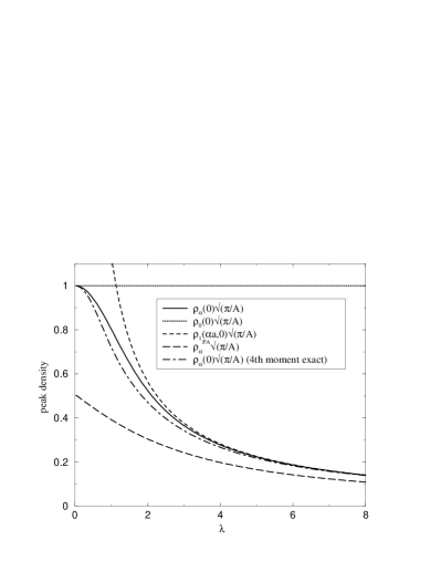
Figure 4: Graph of the peak values of the density $\rho_{\alpha}(0)$, Eq. (LABEL:poigoe), as a function of the transition parameter $\lambda$, Eq. (37). For comparison we also show the limiting cases $\rho_{0}(0)$, Eq. (29), and $\rho_{1}(\alpha a,0)$, Eq. (39), as well as an interpolation formula given by Persson and Åberg Persson and Åberg (1995) $\rho_{\alpha}^{\rm{PA}}$, Eq (50). Finally, we show $\rho_{\alpha}(0)$ calculated using Eq. (LABEL:poigoe) modified in accordance with Eqs. (48) and (49).

In Fig. 3 we show the improvement to the ALD obtained by using Eqs. (48) and (49) in Eq. (LABEL:poigoe) for the worst case of Fig. 1 ($\alpha$=0.05). We see that the modified formula gives the ALD essentially exactly.

In Fig. 4 we show the peak value of the density of states as a function of $\lambda$ (see figure caption). We see that Eq. (LABEL:poigoe) in both its modified and unmodified versions agree at the $\lambda$=0 limit. We also see that both versions of Eq. (LABEL:poigoe) reach the $N\to\infty$ limit [Eq. (39)] at roughly the same value of $\lambda$ ($\lambda$$\approx$6). However the two versions deviate from each other in the transition region, the largest difference occuring around $\lambda$$\approx$1.5 ($\alpha$$\approx$0.05 for $N$=1000). Also shown for comparison is the interpolation formula for the ALD of Persson and Åberg Persson and Åberg (1995):

$$\rho_{\alpha}^{\rm{PA}}=\frac{N^{\frac{1}{2}}}{4\alpha N^{\frac{1}{2}}+7N^{-1.5\alpha}}.$$ (50)

V The transition GOE to $m$ GOEs

Figure 5: Graph of $\rho_{\alpha}(E)$ illustrating the transition 3 GOEs to GOE. The three block have size $M_{1}$=50, $M_{2}$=400 and $M_{3}$=550. The densities for $\alpha$= 0, 0.7, 1.0 are shown. The calculations where performed with $A$=$N/4$ for which the radius of the Wigner semi-circle is $a$=2. The solid lines were calculated using Eq. (58) and the dotted histograms by numerical diagonalizing an ensemble of 100 matrices.

We now calculate the ALD for the transition from the GOE to a superposition of $m$ GOEs. To proceed we again consider an ensemble of matrices of the form of Eq. (4). Now $H_{0}$ is a block diagonal matrix consisting of $m$ blocks whose dimensions are $M_{i}$, $i=1,2,...,m$, with $\sum\limits_{i=1}^{m}M_{i}=N$. The elements of $H_{0}$ have zero mean and variances given by Eq. (3). We define $H_{1}$ to be zero where $H_{0}$ is non-zero and elsewhere its elements have zero mean and variances given by Eq. (5).

To obtain a formula for the ALD we note that

$$\overline{\mathop{\rm tr}H^{2}} = \sum_{j,k=1}^{N}\overline{H_{jk}^{2}}$$ (51)

$$= N^{2}\sum_{i=1}^{m}\frac{M_{i}}{N}\sigma_{i}^{2}$$ (52)

with

$$\sigma_{i}^{2}=\frac{1}{4A}\left[\frac{M_{i}}{N}+\alpha^{2}(1-\frac{M_{i}}{N})\right].$$ (53)

Considering a single line of $H$ the $\sigma_{i}^{2}$ consist of a term which is the product of the variance of a single non-zero element of $H_{0}$ with the probability for being in block $i$ plus a term which is the product of the variance of a single non-zero element of $H_{1}$ with the probability for being outside block $i$. In the sum in Eq. (52) the $\sigma_{i}^{2}$ are weighted with the fraction of lines which find themselves in block $i$.

For the fourth power of $H$ we find

$$\overline{\mathop{\rm tr}H^{4}} = 2\sum_{j,k,l=1}^{N}\overline{H_{jk}^{2}}\overline{H_{jl}^{2}}$$ (54)

$$= 2\sum_{j=1}^{N}\left[\sum_{k=1}^{N}\overline{H_{jk}^{2}}\right]^{2}$$ (55)

$$= 2N^{3}\sum_{i=1}^{m}\frac{M_{i}}{N}\sigma_{i}^{4}.$$ (56)

Although the authors were unable to obtain an equation analogous to Eq. (55) for higher powers of $H$, Eqs. (52) and (56) strongly suggest that

$$\overline{\mathop{\rm tr}H^{2s}}\simeq C_{s}N^{s+1}\sum_{i=1}^{m}\frac{M_{i}}{N}\sigma_{i}^{2s},$$ (57)

for large $N$.

Substituting Eq (57) into Eq. (12) and again using Eqs. (17), (7) and (19) we obtain

$$\rho\left(E\right)=\sum_{i=1}^{m}\frac{M_{i}}{N}\rho_{1}\left(a_{i},E\right),$$ (58)

where $\rho_{1}$ is given by Eq. (20) and

$$a_{i} = a^{2}\left[\frac{M_{i}}{N}+\alpha^{2}(1-\frac{M_{i}}{N})\right]$$ (59)

$$= \frac{1}{A}\left[M_{i}+\lambda^{2}(1-\frac{M_{i}}{N})\right].$$ (60)

From Eq. (58) it follows that the CLD, Eq. (21), is given by

$$x\left(E\right)=\sum_{i=1}^{m}\frac{M_{i}}{N}x_{1}\left(a_{i},E\right),$$ (61)

with $x_{1}$ given by Eq. (22).

In Fig. 5, we compare Eq. (58) for the ALD with numerical simulations for several values of the $\alpha$ (see figure caption for details) and excellent agreement is obtained.

VI Conclusion

In conclusion, by assuming that terms containing patterns of unlinked binary associations dominate the the averages of traces of powers of matrices, we have derived formulas for the average level density for two deformations of the Gaussian orthogonal ensemble. The first describes the transition from the Gaussian orthogonal ensemble to the Poisson ensemble and the second the transition from the GOE to $m$ GOEs. The formula obtained are in excellent agreement with numerical simulations.