Hydrodynamic Approaches to
Relativistic Heavy Ion Collisions

Abstract

We give a short review about the hydrodynamic model and its application to the elliptic flow phenomena and the pion interferometry in relativistic heavy ion collisions.

24.10.Nz, 25.75.-q

1 Introduction

First data reported by the STAR Collaboration at RHIC [1] has a significant meaning that the observed large magnitude of elliptic flow for charged hadrons is consistent with hydrodynamic predictions [2]. This suggests that large pressure possibly in the partonic phase is built at the early stage ($\tau\sim 0.6$ fm/$c$) in Au+Au collisions at $\sqrt{s_{NN}}=$ 130 and 200 GeV. This situation at RHIC is in contrast to that at lower energies such as AGS or SPS where hydrodynamics always overpredicts the data [3]. Moreover, this also suggests that the effect of the viscosity in the QGP phase is remarkably small and that the QGP is almost a perfect fluid [4]. Hadronic transport models are very good to describe experimental data at lower energies, while they fail to reproduce such large values of elliptic flow parameter at RHIC (see, e.g., Ref. [5]). So the importance of hydrodynamics is rising in heavy ion physics. After the first STAR data were published [1], other groups at RHIC have also obtained the data concerning with flow phenomena [6].

Contrary to the success of the hydrodynamics to describe the elliptic flow, many dynamical models including hydrodynamics cannot reproduce the HBT radii [7, 8, 9]. It is known as the “HBT puzzle”.

To understand these experimental data, hydrodynamic analyses are performed extensively [10, 11]. In this short review, we highlight several results mainly on elliptic flow and on the HBT radii from hydrodynamic calculations.

2 Basics of Ideal Hydrodynamics

Hydrodynamic equations represent the energy-momentum conservations $\partial_{\mu}T^{\mu\nu}=0$. In the ideal hydrodynamics, the energy-momentum tensor becomes $T^{\mu\nu}=(e+P)u^{\mu}u^{\nu}-Pg^{\mu\nu}$, where $e$ is the energy density, $P$ is the pressure, and $u^{\mu}$ is the four fluid velocity. When there are conserved quantities such as the baryon number or the number of chemically frozen hadrons, one needs to solve the continuity equations $\partial_{\mu}n_{i}^{\mu}=0$ together with the hydrodynamic equations. In order to close the system of partial differential equations, the equation of state (EoS) $P(e,n_{i})$ is needed. The naive applicability conditions of ideal hydrodynamics are that the mean free path among the particles is much smaller than the typical size of the system and that the system keeps local thermal equilibrium during expansion. From these conditions, one cannot use hydrodynamics for initial collisions, final free streaming and high $p_{T}$ ($\stackrel{{\scriptstyle>}}{{\sim}}$  2 GeV/$c$) particles. So one needs an interface between the pre-thermalisation stage and the hydrodynamic stage at the initial time. Moreover, the system eventually breaks up and cannot keep thermalisation at the later stage. This means a prescription of freezeout is needed in the hydrodynamic model in evaluating the particle spectra. Therefore one needs another interface between the hydrodynamic stage and the free streaming stage. In what follows, we discuss particularly equations of state, initial conditions and freezeout prescriptions used in the literature.

2.1 Equation of State

The main ingredient of the hydrodynamic model is the equation of state (EoS) for thermalised matter produced in heavy ion collisions. Ideally, one uses the EoS taken from the first principle calculations of QCD, namely, lattice QCD simulations [12]. More practically, one can use the resonance gas model for the hadron phase and the massless free parton gas for the QGP phase. By matching these two models at the critical temperature, one obtains the first order phase transition model with a latent heat $\sim$1 GeV/fm³. In the mixed phase at $n_{B}=0$, the sound velocity $c_{s}^{2}={\partial P}/{\partial e}$ is vanishing. Recent lattice QCD simulations tell us that the phase transition seems to be crossover in vanishing baryonic chemical potential. Discontinuity of the thermodynamic variables does not exist in the crossover phase transition. It should be emphasized, however, that the energy density and the entropy density increase more rapidly than the pressure in the vicinity of the phase transition region $\Delta T\sim 0.1T_{c}$. This also leads to very small sound velocity near the phase transition region. Therefore it is very hard in general to find flow observables which distinguish the crossover phase transition with a rapid change of the thermodynamic variables from the first order phase transition.

2.2 Initial Condition

Once initial conditions are assigned, one can numerically simulate the space-time evolution of thermalised matter which is governed by hydrodynamic equations. Usually, initial conditions are parametrised based on some physical assumptions. Transverse profile of the energy/entropy density is assumed to be proportional to the number density of participants $\rho_{\mathrm{part}}$, the number density of binary collisions $\rho_{\mathrm{coll}}$ or linear combination of them. Initial transverse flow is usually taken to be vanishing.

On the other hand, one can introduce model calculations to obtain the initial condition of hydrodynamic simulations. Event generators can be used to obtain the energy density distribution at the initial time. Recently, the SPheRIO group employs an event generator NeXus and takes an initial condition from this model in the event-by-event basis [13, 14]. The resultant energy density distribution in the transverse plane has highly bumpy structures [13, 15]. Smooth initial conditions used in the conventional hydrodynamic simulations are no longer expected in one event. Another important example which is relevant at very high collision energies is an initial condition taken from the Colour Glass Condensate picture. See Ref. [16] for recent calculations.

2.3 Freezeout

Conventional prescription to obtain the invariant momentum spectra from the hydrodynamic simulations is to employ the Cooper-Frye formula [17]. The physical picture described by the Cooper-Frye formula is sometimes called “sudden freezeout” since the mean free path is suddenly changed from zero to infinity through a thin freezeout hypersurface. Instead of using this, one can use a hadronic cascade model to describe the space-time evolution of hadrons [18, 19]. The mean free path among hadrons is finite and depends on hadronic species. Hence, one can describe a continuous freezeout picture through hadronic transport models. Note that continuous particle emission can be considered within the hydrodynamics [20]. Adoption of hadronic transport models after hydrodynamic evolution of the QGP liquid could refine the dynamical modeling of relativistic heavy ion collisions. However, it is not so easy to connect them in a systematic and proper way [21].

3 Hydrodynamic Results for $v_{2}$

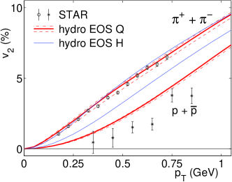
Figure 1: (Left) Transverse momentum dependence of $v_{2}$ for pions and (anti)protons [11] are compared with the STAR data [23] in minimum bias Au+Au collisions at $\sqrt{s_{NN}}=130$ GeV. EoS Q stands for the first order phase transition model, while EoS H stands for the resonance gas model. (Right) $v_{2}$ for charged hadrons as a function of pseudorapidity $\eta$ in Au+Au collisions at $\sqrt{s_{NN}}=130$ GeV [1, 26]. PCE means the EoS of partial chemical equilibrium, whereas CE means the EoS of chemical equilibrium. Figure is taken from Ref. [24].

Assuming the Bjorken flow [22] for the longitudinal direction, one can solve the hydrodynamic equations only in the transverse plane at midrapidity. Systematic studies based on this (2+1)-dimensional hydrodynamic model are performed in Ref. [2]. For the EoS, complete chemical equilibrium is assumed for both the QGP phase and the hadron phase. $p_{T}$ dependences of $v_{2}$ for pions and protons from this model [11] are compared with the STAR data [23] in Fig. 1 (left). By employing the EoS with phase transition, the hydrodynamic model correctly reproduces $v_{2}(p_{T})$ and its mass-splitting behavior below $p_{T}=1$ GeV/$c$. On the other hand, $v_{2}(p_{T})$ for (anti)protons from the resonance gas model does not agree with the data. Although the reason for the difference of the result between these two EoS models is not so clear, the experimental data favors the QGP EoS. Due to the assumption of chemical equilibrium in the hadron phase, this model does not reproduce particle ratio and spectra simultaneously. It is of importance to study whether the agreement with the experimental data still holds even when the assumption of chemical equilibrium in the hadron phase is abandoned [24].

One needs a full 3D hydrodynamic simulation to obtain the rapidity dependence of $v_{2}$. First analysis of $v_{2}(\eta)$ at RHIC based on the full 3D hydrodynamic model is performed in Ref. [24, 25]. Figure 1 (right) shows $v_{2}(\eta)$ for charged hadrons in Au+Au collisions at $\sqrt{s_{NN}}=130$ GeV [1, 26]. Here the initial condition for the energy density is so chosen as to reproduce the pseudorapidity distribution of charged hadrons. Hydrodynamic results are consistent with the experimental data only near the midrapidity while hydrodynamics overpredicts the data in the forward/backward rapidity regions. Multiplicity is not so large in the forward/backward rapidity regions, so equilibration of the system tends to be spoiled.

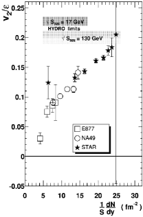
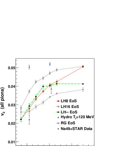
Figure 2: (Left) Excitation function of $v_{2}/\varepsilon$. Figure taken from Ref. [27]. (Right) Excitation function from the hydro+cascade model. Figure taken from Ref. [19].

Figure 2 (left) shows the excitation function of $v_{2}$ compiled by the STAR Collaboration [27]. Hydrodynamic results presented in this figure are based on the same model discussed in Fig. 1 (left). Data points continuously increase with the unit rapidity density at the AGS, SPS and RHIC energies. However, the hydrodynamic response $v_{2}/\varepsilon$ is almost flat or slightly decreases with the multiplicity. The data points seem to reach the “hydrodynamic limit” for the first time at the RHIC energy. The deviation between the hydrodynamic results and the data plots below $(1/S)dN/dy=25$ reminds us the pseudorapidity dependence of elliptic flow in Fig. 1 (right). The deviation might come from a common origin [28]: The small multiplicity both in forward rapidity region at the RHIC energy and at midrapidity at the lower collision energies could cause the partial thermalisation. In the low density limit, $v_{2}$ is actually proportional to the number density [29]. The shape of $v_{2}(\eta)$ data in forward rapidity region looks similar to that of the pseudorapidity distributions [30]. Similarly, data plots of excitation function increase almost linearly with the particle density. These results suggest that thermalisation is not achieved completely in forward rapidity region at the RHIC energy and at midrapidity at the SPS energies.

Figure 2 (right) shows the excitation function from the hydro+cascade (RQMD) model [19] with Bjorken longitudinal flow [22]. Contrary to the conventional hydrodynamic models, freezeout processes are automatically described by the cascade model without any adjustable parameters. The excitation function in the case of the latent heat $\sim 0.8$ GeV/fm³ linearly increases with the multiplicity, which is consistent with the experimental data. The difference from the conventional hydrodynamic results might come from the strong viscosity in the hadron phase within the cascade calculation. It should be noted that $v_{2}(p_{T})$, its mass dependences and particle spectra/ratio at midrapidity are also reproduced by this hybrid model [19].

4 Hydrodynamic Results for HBT Radii

Although many hydrodynamic calculations are already performed, one does not succeed to interpret the HBT puzzle yet. The main reason why the hydrodynamic simulations overestimate the $R_{\mathrm{out}}/R_{\mathrm{side}}$ is the negative value of the correlation between $\tilde{x}_{\mathrm{out}}$ and $\tilde{t}$ which comes from the hydrodynamic source function [11]. Here $\tilde{x}=x-\langle x\rangle$ and the average is taken over the source function. Note that positive $\tilde{x}_{\mathrm{out}}$-$\tilde{t}$ correlation can be obtained dynamically in a transport model [31]. So detailed comparison of this result with hydrodynamic results would be important in understanding the space-time evolution of matter in heavy ion collisions.

As discussed in Sec. 2.3, the conventional hydrodynamics assumes the sudden freezeout which must be far from the realistic situation. The HBT radii reflect the distribution of the final scattering points. So realistic treatment of the final decoupling stage is mandatory.  To remove this unwanted feature in the hydrodynamic model, the continuous particle emission is proposed in Ref. [14, 20]. This prescription naturally gives that larger momentum particles comes from the earlier stage and that smaller momentum particles comes from the later stage. For details of the results, see Ref. [14].

As shown in the previous section, the hydrodynamics with a hadronic cascade model at the late stage reproduces the momentum space of particle spectra from SPS to RHIC energies. This indicates the dilute hadronic gas should not be described by the ideal hydrodynamics. In Ref. [34], a hydro+cascade (UrQMD) approach is employed to calculate the ratio of the pion HBT radii as shown in Fig. 3. In the case of $T_{c}=160$ MeV, the ratio becomes 2.0 around pair transverse momentum $K_{T}=$0.15 GeV/$c$ at hadronization which is much larger than the experimental data $\sim 1$ [7, 8]. Although smearing of freezeout hypersurface by using a hadronic cascade reduces the ratio to 1.4-1.6, it is not enough to reproduce the experimental data.

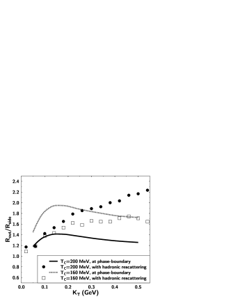
Figure 3: $R_{\mathrm{out}}$/$R_{\mathrm{side}}$ at hadronization (lines) and at freezeout (symbols) from a hydro+cascade approach.

5 Summary and Outlook

The most successful hydrodynamic approach to elliptic flow in relativistic heavy ion collisions is the hybrid model in which the QGP phase is described by the ideal hydrodynamics while the hadron phase is described by a hadronic cascade. However, even within this model, the ratio of the HBT radii is still larger than the data. The Bjorken scaling solution is assumed in the current hydro+cascade models. This means that current hybrid models are available only near midrapidity. Therefore it is desired to develop a model in which a full 3D hydrodynamic simulations combined with a hadronic cascade model. From agreement of excitation function between the hybrid model and the experimental data at midrapidity, the 3D hybrid model is expected to reproduce the pseudorapidity dependence of elliptic flow. It should be emphasised again that the hybrid model has its own problem on the violation of energy momentum conservations between the QGP liquid and the hadron gas. A hybrid simulation which incorporates a proper treatment at the boundary between the QGP phase and the hadron phase is now an open problem.

References

- [1] K.H. Ackermann et al.(STAR Collaboration), Phys. Rev. Lett. 86, 402 (2001).
- [2] P.F. Kolb, P. Huovinen, U. Heinz, H. Heiselberg, Phys. Lett. B 500, 232 (2001); P. Huovinen, P.F. Kolb, U.W. Heinz, P.V. Ruuskanen, S.A. Voloshin, Phys. Lett. B 503, 58 (2001); P.F. Kolb, U.W. Heinz, P. Huovinen, K.J. Eskola, K. Tuominen, Nucl. Phys. A696, 197 (2001).
- [3] C. Alt, et al.(NA49 Collaboration), Phys. Rev. C 68, 034903 (2003); G. Agakichiev et al.(CERES/NA45 Collaboration), Phys. Rev. Lett. 92, 032301 (2004).
- [4] E. Shuryak, J. Phys. G 30, S1221 (2004); D. Teaney, Phys. Rev. C 68, 034913 (2003).
- [5] M. Bleicher, H. Stocker, Phys. Lett. B 526, 309 (2002).
- [6] F. Retière, J. Phys. G 30, S827 (2004).
- [7] C. Adler et al. (STAR Collaboration), Phys. Rev. Lett. 87, 082301 (2001).
- [8] K. Adcox et al. (PHENIX Collaboration), Phys. Rev. Lett. 88, 192302 (2002).
- [9] D. Magestro, these proceedings.
- [10] P. Huovinen, Quark Gluon Plasma 3, eds. R. Hwa, X.N. Wang, World Scientific, Singapore 2003, p. 600.
- [11] P.F. Kolb, U. Heinz, Quark Gluon Plasma 3, eds. R. Hwa, X.N. Wang, World Scientific, Singapore 2003, p. 634.
- [12] F. Karsch, Lect. Notes Phys. 583, 209 (2002).
- [13] T. Osada, C. E. Aguiar, Y. Hama, T. Kodama, nucl-th/0102011; Y. Hama, T. Kodama, O. Socolowski Jr., hep-ph/0407264.
- [14] Y. Hama, these proceedings.
- [15] M. Gyulassy, D.H. Rischke, B. Zhang, Nucl. Phys. A613, 397 (1997).
- [16] T. Hirano, Y. Nara, Nucl. Phys. A 743, 305 (2004).
- [17] F. Cooper, G. Frye, Phys. Rev. D 10, 186 (1974).
- [18] S.A. Bass, A. Dumitru, Phys. Rev. C 61, 064909 (2000).
- [19] D. Teaney, J. Lauret, E.V. Shuryak nucl-th/0110037.
- [20] F. Grassi, Y. Hama, T. Kodama, Phys. Lett. B 355, 9 (1995); O. Socolowski Jr., F. Grassi, Y. Hama, T. Kodama, hep-ph/0405181.
- [21] K.A. Bugaev, Phys. Rev. Lett. 90, 252301 (2003); nucl-th/0401060.
- [22] J.D. Bjorken, Phys. Rev. D 27, 140 (1983).
- [23] C. Adler et al.(STAR Collaboration), Phys. Rev. Lett. 87, 182301 (2001).
- [24] T. Hirano, K. Tsuda, Phys. Rev. C 66, 054905 (2002).
- [25] T. Hirano, Phys. Rev. C 65, 011901 (2001).
- [26] B.B. Back et al.(PHOBOS Collaboration), Phys. Rev. Lett. 89, 222301 (2002).
- [27] C. Adler et al.(STAR Collaboration), Phys. Rev. C 66, 034904 (2002).
- [28] U. Heinz, P. Kolb, J. Phys. G 30, S1229 (2004).
- [29] H. Heiselberg, A.M. Levy, Phys. Rev. C 59, 2716 (1999)
- [30] P.A. Steinberg, Nucl. Phys. A 698, 314c (2002)
- [31] Z.W. Lin, C.M. Ko, S. Pal, Phys. Rev. Lett. 89, 152301 (2002).
- [32] C.Y. Wong, J. Phys. G 29, 2151 (2003).
- [33] J. Kapusta, Y. Li, J. Phys. G 30, S1069 (2004).
- [34] S. Soff, S.A. Bass, A. Dumitru, Phys. Rev. Lett. 86, 3981 (2001).