Many-Body Physics on the Border of Nuclear Stability

Abstract

A brief overview is given of the Continuum Shell Model, a novel approach that extends the traditional nuclear shell model into the domain of unstable nuclei and nuclear reactions. While some of the theoretical aspects, such as role and treatment of one- and two-nucleon continuum states, are discussed more in detail, a special emphasis is made on relation to observed nuclear properties, including definitions of the decay widths and their relation to the cross sections, especially in the cases of non-exponential decay. For the chain of He isotopes we demonstrate the agreement of theoretical results with recent experimental data. We show how the interplay of internal collectivity and coherent coupling to continuum gives rise to the universal mechanism of creating pigmy giant resonances.

1 Continuum Shell Model

Recent progress in physics of weakly bound nuclei and other marginally stable mesoscopic systems requires an adequate many-body theory which would combine the bound states and continuum in a consistent description. Below we show how it can be done. Our formalism of continuum shell model (CSM) follows closely the projection method by Feshbach Feshbach (1958). The many-body states of the system are separated into subspaces ${P}$ and ${Q}$, and the Hamiltonian consists of three parts, $H=H_{QQ}+H_{PP}+H_{PQ}.$ The internal space ${P}$ contains shell model (SM) states with all particles on bound single-particle orbitals, for example $N$-nucleon $m$-scheme Slater determinants, labelled as $|1\rangle$. The external space ${Q}$ contains all states $|c;E\rangle$, labelled by energy $E$ and channel $c$, with some particles in the continuum. These wave functions asymptotically behave as outgoing spherical (Coulomb) waves with respect to one or several single-particle arguments. We solve the Schrödinger equation $H|\alpha;E\rangle=E|\alpha;E\rangle$ within the total ${P}+{Q}$ space where an eigenstate $\alpha$ is a superposition

$$|\alpha;E\rangle=\sum_{1}\alpha_{1}(E)|1\rangle+\sum_{c}\int dE^{\prime}\,\alpha_{c}(E^{\prime};E)|c;E^{\prime}\rangle,$$ (1)

Elimination of external states leads to the effective energy-dependent Hamiltonian that acts within $P$ space,

$${\cal H}(E)=H_{PP}+\Delta(E)-\frac{i}{2}\,W(E)\,.$$ (2)

Here $\Delta(E)$ is a self-energy term coming from virtual excitations into the continuum and $W(E)$ stands for the explicitly non-Hermitian term due to the open decay channels,

$$\langle 1|\Delta(E)|2\rangle=\sum_{c}\,P\int dE^{\prime}\,\frac{{A^{c}_{1}(E^{\prime})}^{*}\,{A^{c}_{2}(E^{\prime})}}{E-E^{\prime}},\quad\langle 1|W(E)|2\rangle=2\pi\sum_{c\,({\rm open})}{A^{c}_{1}(E)}^{*}\,{A^{c}_{2}(E)}.$$ (3)

The amplitude of coupling to the continuum, $A^{c}_{1}(E)$, is introduced as $\,A_{1}^{c}(E)=\langle c;E|H_{QP}|1\rangle\,$. For Eqs. (3) it is assumed for simplicity that the ${P}$ and ${Q}$ spaces are orthogonal, and that for the continuum $H_{QQ}|c;E\rangle=E|c;E\rangle$. Thus, given the effective Hamiltonian (2), the internal solution can be found as

$$\sum_{2}{\cal H}_{12}(E)\alpha_{2}(E)={\cal E}\alpha_{1}(E),$$ (4)

then, using the internal amplitudes $\alpha_{1}(E)$, the continuum part can be restored as

$$\alpha_{c}(E^{\prime};E)=\sum_{1}\,\alpha_{1}(E)\,\frac{A^{c}_{1}(E^{\prime})}{E-E^{\prime}+i0}\,.$$ (5)

The energy dependence of the effective Hamiltonian (2) in this formalism emphasizes the non-exponential nature of decay processes. The experimental observables can be found through the scattering matrix that is expressed via the same Hamiltonian:

$$S^{cc^{\prime}}(E)=\exp(i\xi_{c})\,\left\{\delta^{cc^{\prime}}-\sum_{12}A^{c\ast}_{1}(E)\,\left(\frac{1}{E-{\cal H}(E)}\right)_{12}A^{c^{\prime}}_{2}(E)\right\}\exp(i\xi_{c^{\prime}}),$$ (6)

where $\xi_{c}$ is a smooth scattering phase in channel $c$ coming from features not accounted in the model Hamiltonian.

Equation (4) has no solutions with real eigenvalues ${\cal E}$. This is not surprising since stationary intrinsic states cannot be matched by outgoing continuum states in Eq. (1). However, solutions do exist in the complex energy plane $E\rightarrow{\cal E}$ as Gamow quasistationary states Gamow (1928), where resonance energies are taken as $E_{\rm res}={\rm Re}({\cal E})$ and widths are identified as $\Gamma_{\rm res}=-2{\rm Im}({\cal E})$. The related non-Hermitian eigenvalue problem is discussed in Siegert (1939); Berggren (1968, 1996). This solution for the resonance lies in the foundation of the alternative approach, so-called Gamow Shell Model Michel et al. (2003), where the solution of the non-Hermitian eigenvalue problem finds poles of the scattering matrix (6). The realization of this approach, although well formulated mathematically, is complicated by the difficulty of analytical continuation into the complex plane. In general, the direct solution of Eq. (4) leads to numerous unphysical roots Volya and Zelevinsky (2003a), unless cuts in the complex momentum space are made that separate physical and unphysical regions. The Breit-Wigner formalism gives an alternative definition of a resonance Breit and Wigner (1936), while avoiding transition into the complex energy plain. Here both effective Hamiltonian and scattering matrix are evaluated only on the real energy axis. The resonance energy is determined from the condition that real part in the denominator of scattering matrix vanishes which is equivalent to finding $E_{\rm res}$ as $E_{\rm res}={\rm Re}({\cal E})$, where ${\cal E}=E_{{\rm res}}-(i/2)\Gamma_{{\rm res}}$ is a complex eigenvalue of ${\cal H}(E_{\rm res})$. There is yet another definition of a resonance that is closely related to the experimental cross section when, from a phase shift $\delta$ in a given channel, the resonance width is defined as the phase shift derivative which at the resonance produces the maximum time delay $\tau$,

$$\tau=\frac{2}{\Gamma}=\left.\frac{d\delta(E)}{dE}\right|_{E=E_{{\rm res}}},\quad\left.\frac{d^{2}\delta_{l}(E)}{dE^{2}}\right|_{E=E_{\rm res}}=0\,.$$ (7)

Having defined the resonance region as the energy region of size $\Gamma$ around the resonance energy, all of the above definitions agree if the two conditions are fulfilled: (1) the resonance regions do not overlap; (2) the energy dependence of the effective Hamiltonian in each of the resonance regions is weak and can be ignored. In the realistic cases, when the density of states is high and these conditions are violated, one has to be specific and identify the definition of resonances and widths. In this work we use a Breit-Wigner definition for the width. It is also important that the CSM can be used for calculating the cross sections which leads to direct comparison with experiment. In that case, in contrast to a traditional SM, the large-scale matrix diagonalization is substituted by the matrix inversion needed for Eq. (6).

2 Application to weakly-bound nuclei

In the following application of the CSM we assume that the Hermitian part of the effective Hamiltonian $H_{PP}+\Delta$ is given by the phenomenological SM Hamiltonian and limit $Q$-space to one and two particles in the continuum. Phenomenologically adjusted interactions include corrections from virtual excitations to the continuum $\Delta$. Energy dependence of $\Delta(E)$ is ignored since, unlike the non-Hermitian term $W$, $\Delta$ is not sensitive to thresholds. This choice of the interaction assures that, for the states below decay thresholds, coupling to continuum disappears, $W=0$, and the results of the conventional SM are exactly reproduced.

We assume that the mean field Hamiltonian selected here as a Woods-Saxon potential is responsible for single-particle widths while the additional schematic two-body interaction discussed below is introduced in $H_{PQ}$ to mediate direct two-body decay processes. With $b^{\dagger}(\epsilon)$ defined as a single-particle creation operator in the continuum state with energy $\epsilon$, a one-particle channel with quantum numbers $j$, energy of the particle $\epsilon_{j}$, and the residual nucleus in the state $|\alpha;N-1\rangle$, so that $E=E_{\alpha}+\epsilon_{j}$, is asymptotically labelled as $|c\rangle=b^{\dagger}_{j}(\epsilon_{j})|\alpha;N-1\rangle$. The two-body channel can be expressed similarly, $|c\rangle=b_{j}^{\dagger}(\epsilon)b^{\dagger}_{j^{\prime}}(\epsilon^{\prime})|\alpha;N-2\rangle.$ The first contribution from the continuum comes through a single-particle decay amplitude

$$A^{c}_{1}(E_{\alpha}+\epsilon_{j})=\sum_{\nu}a^{j}_{\nu}(\epsilon_{j})\,\langle\alpha;N-1|b_{\nu}|1;N\rangle,$$ (8)

where the reduced single-particle amplitudes are

$$a^{j}_{\nu}(\epsilon)=\langle 0|b_{\nu}(\epsilon)\,H_{PQ}\,b^{\dagger}_{j}|0\rangle,$$ (9)

and the operators $b^{\dagger}_{\nu}$ create particles on the discrete SM orbitals. If the valence space is small, each single-particle state $\nu$ is uniquely identified by spin-isospin quantum numbers $j$. As a result, the contribution to the effective Hamiltonian from one-body decay is

$$\langle 1|W(E)|2\rangle=2\pi\delta_{12}\sum_{c\,({\rm open})}|a^{j}(\epsilon_{j})|^{2}|\langle\alpha;N-1|b_{j}|1;N\rangle|^{2},$$ (10)

where $E=\epsilon_{j}+E_{\alpha}$.

Being in general a many-body operator, $W$ is effectively reduced to a single-particle form in some important cases. For example, far from thresholds one can ignore the energy dependence and use the closure to simplify the summation in (10),

$$\langle 1|W(E)|2\rangle=2\pi\delta_{12}\sum_{j}|a^{j}|^{2}\,|\langle 1;N|b^{\dagger}_{j}b_{j}|1;N\rangle|^{2}.$$ (11)

$W$ than becomes a one-body operator that assigns a width $\gamma_{j}=2\pi\left|a^{j}\right|^{2}$ to each unstable single-particle state $j=\nu$ and can be combined with the shell model Hamiltonian via complex single-particle energies $e_{\nu}=\epsilon_{\nu}-i\gamma_{\nu}/2.$ The single-particle interpretation of the width is possible when the decay process is not associated with a significant change in the structure from parent to daughter nucleus. The coupling amplitude $a^{j}(\epsilon)$, Eq. (9), is calculated numerically through a one-nucleon scattering problem. Within few MeV above decay thresholds, the energy-dependence of $a^{j}(\epsilon)$ to a good accuracy can be parameterized by the power law consistent with the energy scaling of the width as $\Gamma(\epsilon)\sim\epsilon^{l+1/2}$ where $\epsilon$ is the energy above the threshold and $l$ is the partial wave of the decay channel.

With the one-body interaction used for single-particle decays, the admixture from the two-particle continuum can only appear as a second order contribution,

$$A^{c}_{1}(E)=\sum_{\beta}a^{j}(\epsilon)a^{j^{\prime}}(\epsilon^{\prime})\left(\frac{\langle\alpha|b_{j}|\beta\rangle\,\langle\beta|b_{j^{\prime}}|1\rangle}{E-E_{\beta}-\epsilon}+\frac{\langle\alpha|b_{j^{\prime}}|\beta\rangle\,\langle\beta|b_{j}|1\rangle}{E-E_{\beta}-\epsilon^{\prime}}\right)\,,$$ (12)

that proceeds through an intermediate state $\beta$ of the nucleus with $N-1$ particles (sequential two-body decay). The contribution from this decay to matrix $W$ is

$$\langle 1|W(E)|2\rangle=2\pi\sum_{\alpha,j,j^{\prime}}\int\,d\epsilon\,d\epsilon^{\prime}\,\delta(E-E_{\alpha}-\epsilon-\epsilon^{\prime})\,{A^{c}_{1}(E)}^{*}A^{c}_{2}(E)\,.$$ (13)

The integration over single-particle energies may contain poles corresponding to open one-body decays. We concentrate here on the principal value part that represents off-shell processes. Eqs. (12) and (13) allow for additional simplifications in the near-threshold region. The overall width behaves as $\Gamma\sim E_{k}^{2+l+l^{\prime}}$ where $E_{k}$ is the total available kinetic energy.

In contrast to sequential decay, the amplitude for the direct two-body transition is mediated by the two-body interaction in the $H_{PQ}$ part of the Hamiltonian. To describe this process, a pair amplitude is introduced,

$$A^{c}_{1}(E)=a^{(L)}(\epsilon_{1},\epsilon_{2})\,\,\langle\alpha;N-2|p_{L}|1;N\rangle\,,$$ (14)

where the operator $p_{L}=\{b_{\nu}\otimes b_{\nu^{\prime}}\}_{L}$ removes a pair coupled to quantum numbers $L$. Unlike in the sequential case, direct pair emission conserves only the quantum numbers of the pair. Near thresholds we parameterize direct decay amplitude $a^{(L)}(\epsilon_{1},\epsilon_{2})$ with the appropriate energy dependence that reflects the phase space kinematics of the free-body final state.

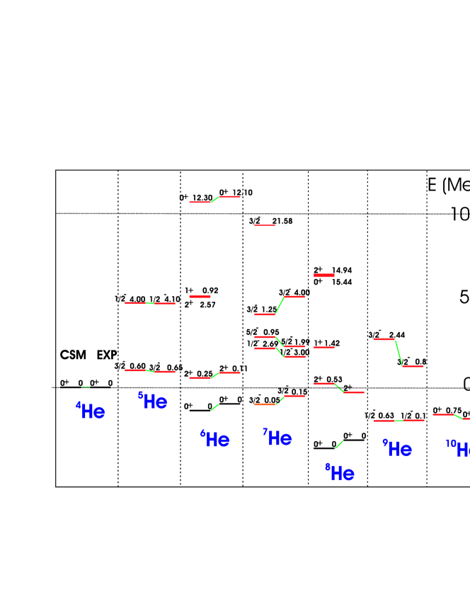
Figure 1: CSM calculation for He isotopes. For each isotope, the CSM result is on the left and experimental value is on the right, energy of each state or resonance is not shown but the energy scale is given on the vertical axis. For each state spin, parity and the decay width in MeV are displayed.

As an example, we consider the $p$-shell chain of helium isotopes from ⁴He to ¹⁰He. The internal space consists of two single-particle levels, $p_{3/2}$ and $p_{1/2}$. The SM interaction and single-particle energies are defined in Cohen and Kurath (1965); Stevenson et al. (1988). For the one-body part of $H_{QQ}$ and $H_{PQ}$ we use the Woods-Saxon potential adjusted for single-particle states in ⁵He. Even at several MeV above threshold, the single-particle widths for the $p$-wave decay from $p_{3/2}$ and $p_{1/2}$ levels to a good accuracy can be described by the parameterizations $\gamma_{3/2}(\epsilon)=0.608\epsilon^{3/2}$ and $\gamma_{1/2}(\epsilon)=0.3652\epsilon^{3/2}$ (all energies in MeV). The sequential two-body decay is computed using Eq. (12) with the near-threshold approximation and the above assumption for the energy dependence of single-particle amplitudes. The calculation with just one-body part in $H_{PQ}$ is inadequate emphasizing the need for the direct two-body decay. This decay is introduced only for pair emission with total angular momentum $L=0$. It is assumed that all $L=0$ neutron pairs couple to the continuum with the same decay amplitude $a^{(L=0)}(\epsilon_{1},\epsilon_{2})$ parameterized as $a^{(L=0)}(\epsilon_{1},\epsilon_{2})={|\epsilon_{1}+\epsilon_{2}|}/{(3.0\sqrt{2\pi})}.$ The numerical constant 3.0, the only parameter of the model, is introduced to describe the unknown strength of the residual two-body interaction needed for two-body decay of ⁶He. With parameters of the model being identified, the full solution proceeds along the chain of isotopes starting from ⁴He, so that at each step the relevant states in the daughter systems are known. For each state in an $N$-particle system, the solution is iterative, energy $E$ is used to determine possible open decay modes into $N-1$ and $N-2$ daughters, then the non-Hermitian part $W(E)$ is constructed, and the full effective Hamiltonian is diagonalized leading to a new complex energy eigenvalue. For each state in the system this procedure is repeated until convergence.

Figure 1 shows the level scheme obtained with the CSM calculation for He isotopes along with experimental data. Beyond good overall agreement, additional fine details can be noted that are in close relation to recent experimental data Korsheninnikov et al. (1999); Rogachev et al. (2003, 2004). For ⁶He the $2^{+}_{1}$ state is well described by the sequential two-body decay into ⁴He. However, the description of the broad first excited $0^{+}$ state requires direct two-body decay, in agreement with the coherent $L=0$ pair-excitation structure of that state Volya et al. (2002). For ⁷He, the CSM confirms the peculiar nature of the 5/2^- state noticed in the experiment Korsheninnikov et al. (1999): this state decays to the excited $2^{+}$ state rather than to the ground state of ⁶He. This is not the case for the neighboring state $1/2^{-}$ that mainly decays to the ground state. Theory and very recent experimental results Rogachev et al. (2004) are in good agreement regarding spectroscopic factors and branching ratios. Additional CSM studies of realistic nuclear cases (the chain of oxygen isotopes) and related discussions can be found in Ref. Volya and Zelevinsky (2004).

3 Low energy branch of giant resonance

The CSM presented here combines structure and reaction physics on the level that goes beyond any perturbative treatment; the unitarity of the scattering matrix is fulfilled automatically. The interesting effects related to the nature of many-body states embedded in the continuum can be noted in the above example of He isotopes. Compared to the conventional SM, the centroids of low-lying decaying states are shifted into continuum, see Ref. Volya and Zelevinsky (2004); in addition, the coupling to the continuum affects mixing of states and their spectroscopic factors.

The drawing schematically shows the spectrum of particle-hole excitations on the right. Due to multipole interaction, the giant collective state (GR) is repelled up in energy. At the same time, coupling to the common particle continuum creates super-radiant (SR) collectivity visible through the particle scattering reaction. The cross section of such a reaction is sketched on the left. Factorized forms of the real interaction and of the coupling to continuum assure collectivity in both GR and decay modes. The dynamics are determined by two multidimensional vectors ${\bf d}=\{d_{n}\}$ and ${\bf A}=\{A_{n}\}$, see text. The multipole interaction shifts the GR accumulating the multipole strength by $\Omega=\lambda{\bf d}^{2}$ along the real energy axis from the unperturbed centroid $\bar{\epsilon}$. The continuum interaction shifts the SR state accumulating the decay width along the imaginary energy axis.

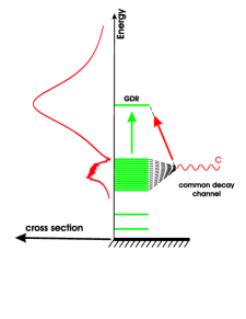
Figure 2:

It was first noted by Dicke Dicke (1954) that strong coupling of two-level atoms to a common radiation field creates superradiant (SR) coherence. The phase transition to the superradiant regime was found to be a universal phenomenon in systems with overlapping resonances ranging in nature from molecular Volya and Zelevinsky (2003b); Pavlov-Verevkin (1988); Flambaum et al. (1996); Persson et al. (2000) to hadronic (pentaquark Auerbach et al. (2004)). The universality of the SR mechanism sokolov89 comes from the factorizable nature of continuum coupling in Eq. (3). With a few continuum channels, the rank of the matrix $W$ is much smaller than the dimension of the intrinsic space. Strong coupling to continuum reorganizes the system in favor of creation of few SR states while the remaining states become long-lived being nearly orthogonal to decay.

Giant resonance (GR) in the response function of the nucleus to a multipole excitation appears as a result of the coherent coupling of particle-hole excitations. In many cases excitation energies of particle-hole configurations lie above the particle separation energy which may lead to another collectivization towards particle emission. We address this interplay in the simplified example Sokolov and Zelevinsky (1990); Sokolov et al. (1997) assuming the effective Hamiltonian

$${\cal H}_{12}=\epsilon_{1}\delta_{12}+\lambda d_{1}d_{2}-\frac{i}{2}A_{1}A_{2}$$ (15)

that contains unperturbed energies, real multipole interaction and interaction through the continuum, see Fig. 2 and the caption for additional discussion.

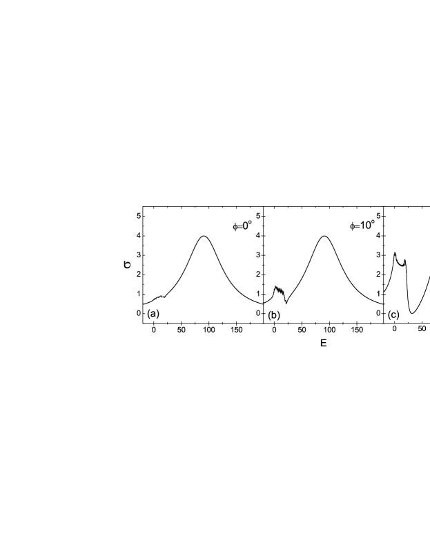
Figure 3: Particle scattering cross section showing the excitation of GR for different angles between GR and SR collectivities.

The interplay of the collective effects depends on the “angle” $\phi$ between the vectors ${\bf d}$ and ${\bf A}$. In the degenerate case, $\epsilon_{n}=\epsilon$, the reaction amplitude is

$$T(E)=\frac{(E-\epsilon-\Omega)\Gamma+\lambda({\bf A}\cdot{\bf d})^{2}}{(E-\epsilon-\Omega)[E-\epsilon+(i/2)\Gamma]+(i/2)\lambda({\bf A}\cdot{\bf d})^{2}}.$$ (16)

In the limits of parallel internal and external couplings, $\phi=0^{\circ}$, the SR and GR collectivizations are coherent, and the experiment will reveal the shifted “Giant Dicke resonance” with full strength and full width $\Gamma={\bf A}^{2}$. This is the case when particle scattering would be most efficient in excitation of the GR. The opposite case of orthogonal couplings, $\phi=90^{\circ}$, will result in a dark collective state with no access to the continuum. Fig. 3 shows a numerical calculation for non-degenerate intrinsic states when the strength and the width are both shared between the displaced GR and the SR in the region of unperturbed excitation energies. With the increasing angle $\phi$ the coupling with continuum becomes more fragmented and less effective in driving the GR; the missing strength develops a low-energy branch revealing the universal mechanism for creating the so-called pigmy giant resonance.

4 Final notes and acknowledgments

We emphasized some of the very recent developments along the road from the nuclear structure and stable nuclei to nuclear reactions and continuum. We were able to highlight only a handful of examples and techniques, a tiny part of a huge modern-day effort. The main message is that the CSM today is no longer a theoretical concept, it is a powerful practical tool capable of describing many-body systems on the border of stability with an impressive quality.

The authors acknowledge support from the U. S. Department of Energy, grant DE-FG02-92ER40750; Florida State University FYAP award for 2004, and National Science Foundation, grant PHY-0244453. Useful discussions with B.A. Brown and G.V. Rogachev are highly appreciated.

References

- Feshbach (1958) Feshbach, H., Ann. Phys., 5, 357 (1958).
- Gamow (1928) Gamow, G., Z. Phys., 51, 204 (1928).
- Siegert (1939) Siegert, A. F. J., Phys. Rev., 56, 750 (1939).
- Berggren (1968) Berggren, T., Nucl. Phys., A109, 265 (1968).
- Berggren (1996) Berggren, T., Phys. Lett., B 373, 1 (1996).
- Michel et al. (2003) Michel, N., Nazarewicz, W., Ploszajczak, M., and Okolowicz, J., Phys. Rev. , C 67, 054311 (2003).
- Volya and Zelevinsky (2003a) Volya, A., and Zelevinsky, V., Phys. Rev. , C 67, 54322 (2003a).
- Breit and Wigner (1936) Breit, G., and Wigner, E., Phys. Rev., 49, 519 (1936).
- Cohen and Kurath (1965) Cohen, S., and Kurath, D., Nucl. Phys., A73, 1 (1965).
- Stevenson et al. (1988) Stevenson, J., et al., Phys. Rev. , C 37, 2220 (1988).
- Korsheninnikov et al. (1999) Korsheninnikov, A. A., et al., Phys. Rev. Lett., 82, 3581–3584 (1999).
- Rogachev et al. (2003) Rogachev, G. V., et al., Phys. Rev., C67, 041603 (2003).
- Rogachev et al. (2004) Rogachev, G. V., et al., Phys. Rev. Lett., 92, 232502 (2004).
- Volya et al. (2002) Volya, A., Zelevinsky, V., and Brown, B., Phys. Rev. , C 65, 054312 (2002).
- Volya and Zelevinsky (2004) Volya, A., and Zelevinsky, V. (2004), submitted to Phys. Rev. Lett.
- Dicke (1954) Dicke, R., Phys. Rev., 93, 99 (1954).
- Volya and Zelevinsky (2003b) Volya, A., and Zelevinsky, V., J. Opt. , B 5, S450 (2003b).
- Pavlov-Verevkin (1988) Pavlov-Verevkin, V., Phys. Rev. , A 129, 168 (1988).
- Flambaum et al. (1996) Flambaum, V., Gribakina, A., and Gribakin, G., Phys. Rev. , A 54, 2066 (1996).
- Persson et al. (2000) Persson, E., Rotter, I., Stöckmann, H.-J., and Barth, M., Phys. Rev. Lett., 85, 2478 (2000).
- Auerbach et al. (2004) Auerbach, N., Zelevinsky, V., and Volya, A., Phys. Lett. , B 590, 45 (2004).
- (22) Sokolov, V., and Zelevinsky, V., Nucl. Phys., A504, 562 (1989).
- Sokolov and Zelevinsky (1990) Sokolov, V., and Zelevinsky, V., Fizika, 22, 303 (1990).
- Sokolov et al. (1997) Sokolov, V., Rotter, I., Savin, D., and Müller, M., Phys. Rev. , C 56, 1031, 1044 (1997).