Effective Field Theories of Light Nuclei

Abstract

Effective field theories have been developed for the description of light, shallow nuclei. I review results for two- and three-nucleon systems, and discuss their extension to halo nuclei.

1 EFFECTIVE FIELD THEORIES

I will remember Göteborg as a clean and ordered town. INPC 2004 was certainly well organized. My talk, too, was about organization.

Nuclear structure involves energies that are much smaller than the typical QCD mass scale, $M_{QCD}\sim 1$ GeV. This is a common situation in physics: an “underlying” theory is valid at a mass scale $M_{\rm hi}$, but we want to study processes at momenta $Q$ of the order of a lower scale $M_{\rm lo}\ll M_{\rm hi}$. Typically, there is “more” at lower energies. How to organize the complexity brought in by the “effective” interactions that will ensure that low-energy observables are described correctly?

Effective Field Theory (EFT) is a framework to construct these interactions systematically, at the same time maintaining desirable general principles such as causality and cluster decomposition. Here I discuss the application of EFT to a class of nuclear systems: those that exhibit poles in the complex momentum plane at a scale much smaller than the pion mass, that is, $M_{\rm hi}\hskip 1.99997pt\raisebox{2.15277pt}{$<$}\raisebox{-3.00003pt}{$\sim$}\hskip 1.99997ptm_{\pi}$. They include two- and three-nucleon systems, and other halo nuclei.

EFT starts with the observation that the effective interactions consist of the sum of all possible interaction terms in a Lagrangian that involves only the fields representing low-energy degrees of freedom. Because of the uncertainty principle, each of these interaction terms can be taken as a local combination of derivatives of the fields. If the “integrating out” of the high-energy degrees of freedom is done appropriately, the effective Lagrangian will have the same symmetries as the underlying theory. The details of the underlying dynamics, on the other hand, are contained in the interaction strengths. The latter depend also on the details of how the low- and high-energy degrees of freedom are separated. This separation requires the introduction of a cutoff parameter $\Lambda$ with dimensions of energy. Both the interaction strengths and the quantum effects represented by loops depend on $\Lambda$. However, the cutoff procedure is arbitrary, so by construction observables are independent of $\Lambda$ (“renormalization-group invariance”). The $T$ matrix for any low-energy process acquires the schematic form

$$T(Q\sim M_{\rm lo})={\cal N}\sum_{\nu=\nu_{\rm min}}^{\infty}c_{\nu}(M_{\rm hi},\Lambda)\left(\frac{Q}{M_{\rm hi}}\right)^{\nu}{\cal F}_{\nu}\left(\frac{Q}{M_{\rm lo}};\frac{\Lambda}{M_{\rm lo}}\right),$$ (1)

where ${\cal N}$ is a common normalization factor, $\nu$ is a counting index starting at some value $\nu_{\rm min}$, the $c_{\nu}$’s are parameters, and the ${\cal F}_{\nu}$’s are calculable functions. We must have

$$\frac{\partial T(Q\sim M_{\rm lo})}{\partial\Lambda}=0.$$ (2)

In order to maintain predictive power in the effective theory it is necessary to truncate the sum in Eq. (1) in such a way that the resulting cutoff dependence can be decreased systematically with increasing order. We call such ordering “power counting”. There are essentially two ways of doing this. One is to carry out the integration of high-energy degrees of freedom explicitly —as it is done in going from QCD to the effective hadronic theory through lattice simulations— and infer the power counting from the sizes of the calculated terms. Another, which we use when we do not know or cannot solve the underlying theory, is to guess the sizes of the effective interactions by assuming that the renormalized interactions are natural, that is, are in order of magnitude given by $M_{\rm hi}$ to a power determined by dimensional analysis. This guess is confirmed a posteriori, by checking renormalization-group invariance and convergence of the truncation after the data is fitted order by order. In some cases, including the ones considered here, there exists a fine-tuning requires a bit more thought.

For the last ten years or so we have been developing EFTs for systems of few nucleons [1]. The goal is to understand traditional nuclear physics from a QCD standpoint. Much of this work has been devoted to the EFT where $M_{\rm hi}\sim M_{QCD}$ and $M_{\rm lo}\sim m_{\pi}$ [1, 2]. In this EFT, pions are explicit degrees of freedom, and (approximate) chiral symmetry plays a crucial role. While in the sector of $A=0,1$ nucleons this “pionful” EFT reduces to well-understood chiral perturbation theory, in the $A\geq 2$ sector power counting is more subtle [3]. Nevertheless, a reasonably successful potential has been constructed [1, 2].

Now, in many situations —in particular, many astrophysical applications— we are interested in reactions at momenta $Q\ll m_{\pi}$. Moreover, as we are going to see, there is interesting nuclear physics in this regime.

2 TWO AND THREE-NUCLEON SYSTEMS

The typical momentum of nucleons in the deuteron is $\aleph_{1}\sim\sqrt{m_{N}B_{d}}\simeq 45$ MeV, which means that the deuteron is an object about three times larger than most of the pion cloud around each nucleon. For the $s_{0}$ virtual bound state, the corresponding scale is even smaller, $\aleph_{0}\sim\sqrt{m_{N}B_{d}^{\prime}}\simeq 8$ MeV. For these states the pionful EFT is an overkill. One can instead consider a much simpler EFT where the meson cloud is represented by a multipole expansion: the Lagrangian contains only nucleon fields with contact interactions.

This “pionless” EFT, for which $M_{\rm hi}\sim m_{\pi}$ and $M_{\rm lo}\sim\aleph$ (with $\aleph$ some average of the $\aleph_{i}$), is now pretty well understood, despite the fact that one needs to account for fine-tuning through the anomalously-small scale $\aleph$. (It seems accidental that $\aleph$ is smaller than a pion scale such as $4\pi f_{\pi}^{2}/m_{N}$, which arises naturally in the pionful EFT [1].) One way to do this is to introduce, in addition to the nucleon spinor/isospinor field $N$ of mass $m_{N}$, two auxiliary —“dimeron”— fields, a scalar/isovector $\mbox{\boldmath$s$}_{0}$ and a vector/isoscalar $\vec{s}_{1}$ with masses $\Delta_{i}$ [4]. (The final results for observables are, of course, independent of the choice of fields.) The most general parity- and time-reversal-invariant Lagrangian is [5, 6, 8, 7, 9]

$${\cal L} = N^{\dagger}\left(i\partial_{0}+\frac{\vec{\overrightarrow{\nabla}}^{\,2}}{2m_{N}}\right)N+\Delta_{0}\,\mbox{\boldmath$s$}_{0}^{\dagger}\cdot\mbox{\boldmath$s$}_{0}+\Delta_{1}\,\vec{s}_{1}^{\,\dagger}\cdot\vec{s}_{1}$$ (3)

$$-\frac{g_{0}}{2}\left[\mbox{\boldmath$s$}_{0}^{\dagger}\cdot N^{T}\sigma_{2}\mbox{\boldmath$\tau$}\tau_{2}N+{\rm H.c.}\right]-\frac{g_{1}}{2}\left[\vec{s}_{1}^{\,\dagger}\cdot N^{T}\tau_{2}\vec{\sigma}\sigma_{2}N+{\rm H.c.}\right]$$

$$-h\left\{g_{0}^{2}N^{\dagger}(\mbox{\boldmath$s$}_{0}\cdot\mbox{\boldmath$\tau$})^{\dagger}(\mbox{\boldmath$s$}_{0}\cdot\mbox{\boldmath$\tau$})N+g_{1}^{2}N^{\dagger}(\vec{s}_{1}\cdot\vec{\sigma})^{\dagger}(\vec{s}_{1}\cdot\vec{\sigma})N\right.$$

$$\left.\qquad+\frac{g_{0}g_{1}}{3}\left[N^{\dagger}(\vec{s}_{1}\cdot\vec{\sigma})^{\dagger}(\mbox{\boldmath$s$}_{0}\cdot\mbox{\boldmath$\tau$})N+{\rm H.c.}\right]\right\}+\ldots,$$

where the $g_{i}$ and $h$ are coupling constants to be determined. In addition to the kinetic terms for the various fields, the Lagrangian contains all interactions between nucleon and auxiliary fields. (Integrating over the auxiliary fields in the path integral results in a completely equivalent form of the EFT, without auxiliary fields and with purely-contact interactions.) Only some of the most important terms are shown explicitly here: those that contribute to the $s$ waves in the two- and three-nucleon systems. The “$\dots$” include terms with more derivatives and contributions to other waves.

2.1 The two-nucleon system

In the two-nucleon ($NN$) system, the full $T$ matrix can be obtained by adding nucleon legs to the full dimeron propagators. The latter consist of insertions of particle bubbles generated by the two-particle/dimeron interaction —see Fig.1— as well as insertions stemming from terms with more derivatives. Since a two-nucleon bubble is ${\cal O}(m_{N}Q/4\pi)$, if $\Delta_{i}={\cal O}(\aleph_{i})$ and $g_{i}^{2}/4\pi={\cal O}(1/m_{N})$, then the bubbles have to be resummed in the $s$ waves [5]. That is, with the dimeron masses fine-tuned, the leading interactions have to be summed to all orders. The $T$ matrix develops poles at $Q\sim\pm i\aleph_{i}$, which correspond to the observed shallow bound states. Higher-derivative interactions are smaller by powers of $Q/M_{\rm hi}$.

Figure 1: The full dimeron propagator (thick shaded line) is obtained by dressing the bare dimeron propagator (double solid line) with particle bubbles (solid lines) to all orders.

The $NN$ $T$ matrix has the form (1) with ${\cal N}=4\pi/\mu M_{\rm hi}$ and $\nu=\sum_{i}V_{i}d_{i}-p+L$, where in a diagram $V_{i}$ is the number of vertices with $d_{i}$ derivatives, $p$ is the number of $s_{0}$ or $s_{1}$ propagators, and $L$ is the number of loops. One can show [5] that it is equivalent order by order to that of the effective-range expansion. $T$ involves in leading order (LO) only the scattering lengths $|a_{i}|\sim 1/\aleph_{i}$; at next-to-leading order (NLO) and next-to-next-to-leading order (NNLO), also the effective ranges $|r_{i}|\sim 1/m_{\pi}$; and so on. The resulting phase shifts [6, 1] converge to empirical values for $Q\hskip 1.99997pt\raisebox{2.15277pt}{$<$}\raisebox{-3.00003pt}{$\sim$}\hskip 1.99997ptm_{\pi}$, examples being shown in Fig. 2. The deuteron binding energy is found to be $B_{d}=1.91$ MeV in NLO, to be compared with the experimental value of 2.22 MeV.

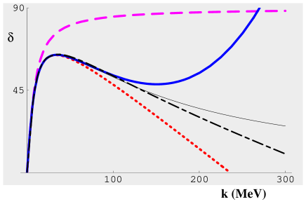
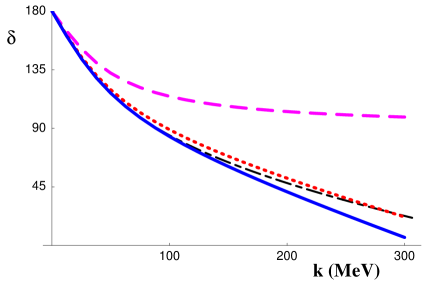
Figure 2: The $s_{0}$ (left) and $s_{1}$ (right) $NN$ phase shifts (in degrees) as functions of the center-of-mass momentum (in MeV). The dash-dotted lines are the Nijmegen phase-shift analysis [10]. Left: the dashed, dotted, and thick solid lines show the EFT results at LO, NNLO, and NNNNLO, respectively, while the thin solid line shows the effective-range result. Right: the dashed, dotted, and thick solid lines show the EFT results at LO, NLO, and NNLO, respectively. From Refs. [1, 6], courtesy of M. Savage.

In addition, many low-energy reactions involving the deuteron have been studied with this EFT —see Ref. [1] for a review.

2.2 The three-nucleon system

The three-nucleon ($3N$) system is more interesting. In all but the $s_{1/2}$ wave, $3N$ forces appear only at high orders, and very precise results for nucleon-deuteron ($Nd$) scattering follow with parameters fully determined from $NN$ scattering [7]. The $s_{3/2}$ phase shift is given as an example in Fig. 3: excellent agreement with data is achieved already at NNLO. In particular, the scattering length is postdicted as $a_{3/2}=6.33\pm 0.10$ fm, to be compared to the experimental value, $6.35\pm 0.02$ fm. One can, thus, do QED-quality nuclear physics with EFT.

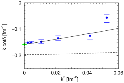
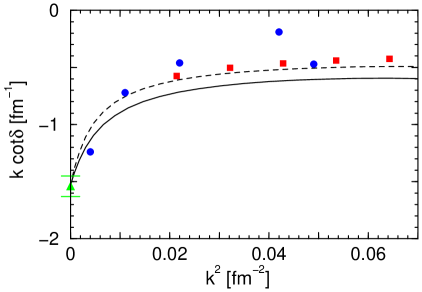
Figure 3: The $s_{3/2}$ (left) and $s_{1/2}$ (right) $Nd$ $K^{-1}$ matrix as function of the square of the center-of-mass momentum (in fm^-2). The points at threshold are from a cold-neutron measurement [11] and the dots from a phase-shift analysis [12]. Left: dashed and solid lines show the EFT results at LO and NNLO, respectively. Right: solid and dashed lines show the EFT results at LO and NLO, respectively, while the squares are the result of a phenomenological potential model [13]. From Refs. [7, 9], courtesy of H. Hammer.

In the $s_{1/2}$ wave, renormalization-group invariance can only be achieved if the $3N$ interactions are also enhanced by two powers of $\aleph^{-1}$ [8, 9]. In this channel, a single non-derivative $3N$ interaction appears in LO, and higher-derivative interactions are smaller by powers of $Q/M_{\rm hi}$. To NLO there is only one parameter not fixed by $NN$ observables —$h$ in Eq. (3)). It can be fixed by, say, the $s_{1/2}$ $Nd$ scattering length, and as a function of the cutoff it displays an unusual, limit-cycle behavior. The resulting energy dependence of $s_{1/2}$ $Nd$ scattering comes out very well [9], see Fig. 3. Likewise, the triton binding energy is found to be $B_{t}=8.31$ MeV in NLO, to be compared with the experimental value of 8.48 MeV.

This EFT simplifies the treatment of light nuclei, but the application to larger nuclei still faces computational challenges. (For the first attack on the four-body system, see Refs. [14, 15].) One would like to devise further simplifications in order to extend EFTs to larger nuclei. As a first step, we can specialize to very low energies where clusters of nucleons behave coherently. Even though many interesting issues of nuclear structure are missed, we can at least describe anomalously-shallow (“halo”) nuclei and some reactions of astrophysical interest.

3 HALOS

I define a halo system as one that contains two momentum scales:

• $M_{\rm hi}\sim\sqrt{m_{N}E_{\rm core}}$, associated with the excitation energy $E_{\rm core}$ of a tight cluster of nucleons (“core”);

• $M_{\rm lo}\sim\sqrt{m_{N}E_{\rm halo}}$, associated with the energy $E_{\rm halo}$ for the attachment or removal of one or more (“halo”) nucleons.

These systems exhibit shallow $S$-matrix poles, either on the imaginary axis (bound states) or elsewhere in the complex momentum plane (resonances). With this definition, the deuteron and the triton are two- and three-body halo systems, respectively. In these cases the core is a single nucleon, $E_{\rm core}\sim m_{\pi}^{2}/m_{N}$, while $E_{\rm halo}\sim B_{d}$ ($B_{t}$) for the deuteron (triton). The next-simplest examples involve a ⁴He core, for which $E_{\rm core}\simeq 20$ MeV. In contrast, the removal energy for two neutrons from ⁶He is $E_{\rm halo}\simeq 1$ MeV [16], making this a three-body halo nucleus. It is interesting that ⁵He is not bound. However, the total cross section for neutron-alpha ($n\alpha$) scattering has a prominent bump at $E_{\rm halo}\sim 1$ MeV, usually interpreted as a shallow $p_{3/2}$ resonance [16]. In addition, reactions involving more complex nuclei are frequently characterized by shallow resonances that are narrow, corresponding to poles near the real momentum axis.

It is natural to generalize the EFT to describe shallow two-body resonances [17, 18], as a step before tackling three-body halo nuclei. Here, for concreteness, I consider $n\alpha$ scattering, which will fix the $N\alpha$ effective interactions, necessary for a future study of ⁶He.

Now, in addition to a nucleon field, I need to consider also a scalar/isoscalar $\phi$ field to represent the ⁴He core of mass $m_{\alpha}$. I also introduce isospinor dimeron fields $s$, $d$, $t$, etc. with masses $\Delta_{0+}$, $\Delta_{1-}$, $\Delta_{1+}$, etc., which can be thought of as bare fields for the various $N\alpha$ channels: $s_{1/2}$, $p_{1/2}$, $p_{3/2}$, etc., which I denote $0+$, $1-$, $1+$, etc. The most general parity- and time-reversal-invariant Lagrangian is [17, 18]

$${\cal L} = \phi^{\dagger}\left(i\partial_{0}+\frac{\overrightarrow{\nabla}^{\,2}}{2m_{\alpha}}\right)\phi+N^{\dagger}\left(i\partial_{0}+\frac{\overrightarrow{\nabla}^{\,2}}{2m_{N}}\right)N+t^{\dagger}\left(i\partial_{0}+\frac{\overrightarrow{\nabla}^{\,2}}{2(m_{\alpha}+m_{N})}+\Delta_{1+}\right)t$$ (4)

$$+\frac{g_{1+}}{2}\bigg{\{}t^{\dagger}\vec{S}^{\,\dagger}\cdot\bigg{[}N\overrightarrow{\nabla}\phi-(\overrightarrow{\nabla}N)\phi\bigg{]}+{\rm H.c.}\bigg{\}}$$

$$+\Delta_{0+}\,s^{\dagger}s+g_{0+}\bigg{[}s^{\dagger}N\phi+\phi^{\dagger}N^{\dagger}s\bigg{]}+g_{1+}^{\prime}t^{\dagger}\left(i\partial_{0}+\frac{\overrightarrow{\nabla}^{\,2}}{2(m_{\alpha}+m_{N})}\right)^{2}t+\ldots,$$

in a notation similar to the one used in Eq. (3), where additionally the $S_{i}$’s are standard $2\times 4$ spin-transition matrices connecting states with total angular momentum $j=1/2$ and $j=3/2$. Again, of all possible interactions among nucleon, alpha and auxiliary fields, only some of the most important terms are shown explicitly here: those that contribute to the $p_{3/2}$ and $s_{1/2}$ partial waves. The “$\dots$” include terms with more derivatives and contributions to other waves.

The $N\alpha$ $T$ matrix can be obtained from the full dimeron propagators by attaching external nucleon and alpha legs. The bubbles in the dressing of dimeron propagators —see Fig.1 again— now represent the propagation of a nucleon and an alpha particle.

3.1 Low energies

A bare dimeron propagator can generate two shallow real poles provided its $\Delta$ is very small: I take $\Delta_{1+}\sim M_{\rm lo}^{2}/\mu$ (where $\mu$ is the $N\alpha$ reduced mass). The bubbles introduce unitarity corrections, which can dislocate the poles to the lower half-plane. The resonance will be narrow if the EFT is perturbative in the coupling $g_{1+}$. This will be so if $g_{1+}^{2}/4\pi\sim 1/M_{\rm hi}\mu^{2}$, in which case a loop is suppressed by $M_{\rm lo}/M_{\rm hi}$. Higher-derivative terms will also be perturbative if their strengths scale with $M_{\rm hi}$ according to their mass dimensions. Likewise, parameters in waves without shallow resonances will be given solely in terms of $M_{\rm hi}$, e.g. $\Delta_{0+}\sim M_{\rm hi}$. This EFT then describes a shallow, narrow resonance with a single fine-tuned parameter $\Delta_{1+}$.

With this scaling, the $N\alpha$ $T$ matrix has the form (1) with ${\cal N}=4\pi/\mu M_{\rm hi}$ and $\nu=\sum_{i}V_{i}d_{i}-2p+L$, where now $p$ is the number of $1+$ propagators. As a consequence, $T$ involves in LO the scattering “lengths” $|a_{0+}|\sim 1/M_{\rm hi}$ and $|a_{1+}|\sim 1/M_{\rm hi}M_{\rm lo}^{2}$, and the effective “range” $|r_{1+}|\sim M_{\rm hi}$ only; at NLO, the unitarity corrections in the same $0+$ and $1+$ waves; at NNLO, $|r_{0+}|\sim 1/M_{\rm hi}$, the shape parameter $|{\cal P}_{1+}|\sim M_{\rm hi}^{3}$, and $|a_{1-}|\sim 1/M_{\rm hi}^{3}$; and so on.

We fit the EFT parameters to an $n\alpha$ phase-shift analysis [19], and find $M_{\rm hi}\sim 100$ MeV and $M_{\rm lo}\sim 30$ MeV. The results [18] for the total and differential $n\alpha$ cross sections are compared with data in Fig. 4. The data are reproduced up to neutron energies of about $E_{N}\approx 0.5$ MeV in LO and $0.8$ MeV in NNLO. (Interestingly, the NLO result worsens the description of the data.) The expansion fails in the immediate neighborhood of the resonance.

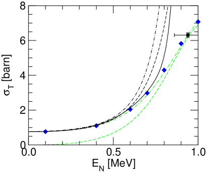
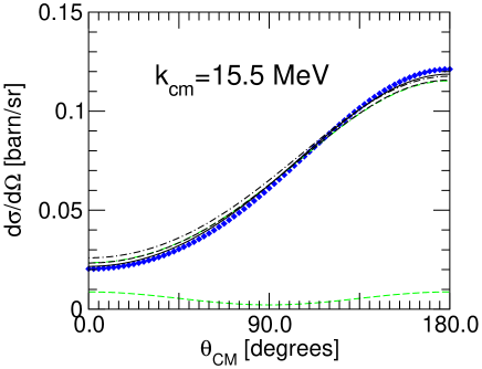
Figure 4: Cross sections for $n\alpha$ scattering below the $p_{3/2}$ resonance. Left: total cross section (in barns) as a function of the neutron kinetic energy (in MeV) in the $\alpha$ rest frame. Right: differential cross section (in barns/sr) as a function of the center-of-mass scattering angle $\theta_{cm}$ (in degrees) at a center-of-mass momentum of $k_{cm}=15.5$ MeV. The diamonds are evaluated data [20], and the black squares are experimental data [21]. The dashed, dash-dotted, and solid black lines show the EFT result without resummation at LO, NLO, and NNLO, respectively. The gray dashed and dash-dotted lines show the EFT result with resummation at LO and NLO, respectively. From Ref. [18].

3.2 Around the resonance

The reason for this failure is easy to understand. In a momentum region of ${\cal O}(M_{\rm lo}^{2}/M_{\rm hi})$ around the resonance there is a cancellation in the denominator of the $1+$ propagator, bubbles have to be resummed to all orders, and the $1+$ propagator is enhanced by a factor of ${\cal O}(M_{\rm hi}/M_{\rm lo})$. In this region, the $N\alpha$ $T$ matrix still has the form (1) but now $\nu=\sum_{i}V_{i}d_{i}-3p+L$. The corresponding results for the total and differential cross sections with data in Fig. 5. The success of this resummed NLO description is evident throughout the low-energy region. (Note that an additional resummation of the $1-$ propagator, which would be necessary if there was a shallow resonance in this channel, as sometimes claimed, does not seem to improve the results significantly.) The description of the phase shifts themselves also comes out pretty well, see Ref. [17].

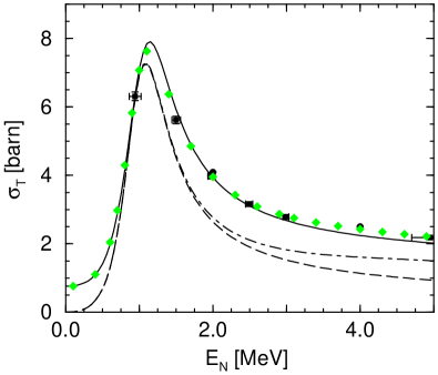
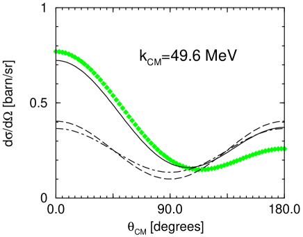
Figure 5: Cross sections for $n\alpha$ scattering around the $p_{3/2}$ resonance. Left: total cross section (in barns) as a function of the neutron kinetic energy (in MeV) in the $\alpha$ rest frame. Right: differential cross section (in barns/sr) as a function of the center-of-mass scattering angle $\theta_{CM}$ (in degrees) at a center-of-mass momentum of $k_{CM}=49.6$ MeV. The diamonds are evaluated data [20], and the black squares are experimental data [21]. The dashed and solid lines show the EFT resummed results at LO and NLO, respectively. (The dash-dotted line shows the LO result in a modified power counting where the $1-$ partial wave is promoted to leading order.) From Ref. [17].

4 OUTLOOK

I have considered here only nuclear shallow states. However, the ideas discussed above are much more general. These EFTs can immediately be extended to other physical systems that contain shallow bound states, such as certain molecules [8, 14, 22]. Apart from specific applications, these EFTs have two interesting generic features that lend them some intrinsic mathematical interest as well. First, they are the simplest theories where short-distance physics produces non-perturbative structures at low energy. Second, the non-perturbative character of the resulting renormalization shows unique features, such as limit cycles. Much more work is possible along these lines —see, e.g. Ref. [23].

More within the scope of this conference, there is certainly reason to push these EFTs in the direction of heavier nuclei. This is in fact just the very beginning of halo EFT. The next step is to use the $N\alpha$ interactions determined from $N\alpha$ scattering [17] and the $NN$ interactions determined from $NN$ scattering [1, 6] to calculate the halo ⁶He as a ${}^{4}{\rm He}+n+n$ system [24], the same way we successfully described triton as a $p+n+n$ system [9]. But clearly the theory can be applied to reactions involving any halo nucleus. For example, to the extent that ⁸B can be regarded as a halo, the reaction $p+\,^{7}{\rm Be}\to\,^{8}{\rm B}+\gamma$ can be analyzed as was $p+n\to d+\gamma$ [1, 6]. This could become, I hope, a useful, systematic approach to physics near the driplines.

References

- [1] P.F. Bedaque and U. van Kolck, Ann. Rev. Nucl. Part. Sci. 52 (2002) 339; S.R. Beane, P.F. Bedaque, W.C. Haxton, D.R. Phillips, and M.J. Savage, nucl-th/0008064; U. van Kolck, Prog. Part. Nucl. Phys. 43 (1999) 337.
- [2] U.-G. Meißner, plenary talk at this conference, nucl-th/0409028.
- [3] S.R. Beane, P.F. Bedaque, M.J. Savage, and U. van Kolck, Nucl. Phys. A700 (2002) 377; A. Nogga, R.G.E. Timmermans, and U. van Kolck, in preparation.
- [4] D.B. Kaplan, Nucl. Phys. B494 (1997) 471.
- [5] U. van Kolck, hep-ph/9711222, in A. Bernstein, D. Drechsel, and T. Walcher (eds.) Proceedings of the Workshop on Chiral Dynamics 1997, Theory and Experiment, Springer-Verlag, Berlin, 1998; Nucl. Phys. A645 (1999) 273; D.B. Kaplan, M.J. Savage, and M.B. Wise, Phys. Lett. B424 (1998) 390; J. Gegelia, nucl-th/9802038.
- [6] J.-W. Chen, G. Rupak, and M.J. Savage, Nucl. Phys. A653 (1999) 386.
- [7] P.F. Bedaque and U. van Kolck, Phys. Lett. B428 (1998) 221; P.F. Bedaque, H.-W. Hammer, and U. van Kolck, Phys. Rev. C58 (1998) R641; F. Gabbiani, P.F. Bedaque, and H.W. Grießhammer, Nucl. Phys. A675 (2000) 601.
- [8] P.F. Bedaque, H.-W. Hammer, and U. van Kolck, Phys. Rev. Lett. 82 (1999) 463; Nucl. Phys. A646 (1999) 444.
- [9] P.F. Bedaque, H.-W. Hammer, and U. van Kolck, Nucl. Phys. A676 (2000) 357; H.-W. Hammer and T. Mehen, Phys. Lett. B516 (2001) 353; P.F. Bedaque, G. Rupak, H.W. Grießhammer, and H.-W. Hammer, Nucl. Phys. A714 (2003) 589.
- [10] V.G.J. Stoks, R.A.M. Klomp, M.C.M. Rentmeester, and J.J. de Swart, Phys. Rev. C48 (1993) 792.
- [11] W. Dilg, L. Koester, and W. Nistler, Phys. Lett. B36 (1971) 208.
- [12] W.T.H. van Oers and J.D. Seagrave, Phys. Lett. B24 (1967) 562; A.C. Philips and G. Barton, Phys. Lett. B28 (1969) 378.
- [13] A. Kievsky, S. Rosati, W. Tornow, and M. Viviani, Nucl. Phys. A607 (1996) 402.
- [14] L. Platter, H.-W. Hammer, and U.-G. Meißner, cond-mat/0404313.
- [15] L. Platter, H.-W. Hammer, and U.-G. Meißner, nucl-th/0409040.
- [16] D.R. Tilley, H.R. Weller, and G.M. Hale, Nucl. Phys. A541 (1992) 1.
- [17] C.A. Bertulani, H.-W. Hammer, and U. van Kolck, Nucl. Phys. A712 (2002) 37.
- [18] P.F. Bedaque, H.-W. Hammer, and U. van Kolck, Phys. Lett. B569 (2003) 159.
- [19] R.A. Arndt, D.L. Long, and L.D. Roper, Nucl. Phys. A209 (1973) 429.
- [20] Evaluated Nuclear Data Files, National Nuclear Data Center, Brookhaven National Laboratory (http://www.nndc.bnl.gov/).
- [21] B. Haesner et al., Phys. Rev. C28 (1983) 995; M.E. Battat et al., Nucl. Phys. 12 (1959) 291.
- [22] H.-W. Hammer, Nucl. Phys. A737 (2004) 275.
- [23] S.D. Głazek and K.G. Wilson, Phys. Rev. Lett. 89 (2002) 230401; A. Morozov and A.J. Niemi, Nucl. Phys. B666 (2003) 311; A. LeClair, J.M. Román, and G. Sierra, hep-th/0312141; A. LeClair and G. Sierra, hep-th/0403178.
- [24] H.-W. Hammer and U. van Kolck, in progress.