Hydrodynamic afterburner for the CGC at RHIC

Abstract

Firstly, we give a short review about the hydrodynamic model and its application to the elliptic flow phenomena in relativistic heavy ion collisions. Secondly, we show the first approach to construct a unified model for the description of the dynamics in relativistic heavy ion collisions.

1 A Short Review on Elliptic Flow from Hydrodynamic models

First data reported by the STAR Collaboration at RHIC [1] has a significant meaning that the observed large magnitude of elliptic flow for charged hadrons is consistent with hydrodynamic predictions [2]. This suggests that large pressure possibly in the partonic phase is built at the early stage ($\tau\sim 0.6$ fm/$c$) in Au+Au collisions at $\sqrt{s_{NN}}=$ 130 and 200 GeV. This situation at RHIC is in contrast to that at lower energies such as AGS or SPS where hydrodynamics always overpredicts the data [3]. Moreover, this also suggests that the effects of the viscosity in the QGP phase is remarkably small and that the QGP is almost a perfect fluid [4]. Hadronic transport models are very good to describe experimental data at lower energies, while they fail to reproduce such large values of elliptic flow parameter at RHIC (see, e.g., Ref. [5]). So the importance of hydrodynamics is rising in heavy ion physics. After the first STAR data were published [1], other groups at RHIC have also obtained the data concerning with flow phenomena [6]. To understand these experimental data, hydrodynamic analyses are also performed extensively [7, 8]. In this short review, we highlight several results on elliptic flow from hydrodynamic calculations.

1.1 Why elliptic flow?

Elliptic flow is very sensitive to the degree of secondary interactions [9]. The indicator of momentum anisotropy is the second harmonic coefficient of azimuthal distributions [10]

$$v_{2}(p_{T},y) = \frac{\int d\phi\cos(2\phi)\frac{dN}{p_{T}dp_{T}dyd\phi}}{\int d\phi\frac{dN}{p_{T}dp_{T}dyd\phi}}=\langle\cos(2\phi)\rangle.$$ (1)

For recent progress of higher harmonics, see Refs. [11, 12]. The spatial anisotropy

$$\varepsilon=\frac{\langle y^{2}-x^{2}\rangle_{s}}{\langle x^{2}+y^{2}\rangle_{s}},\quad\langle\cdots\rangle_{s}=\frac{\int\cdots e(\tau,x)d^{3}x}{\int e(\tau,x)d^{3}x}$$ (2)

at the initial time is a seed of the momentum anisotropy. Within the hydrodynamic picture, pressure gradient along the $x$-axis is larger than the $y$-axis in non-central collisions. Here the direction of $x$-axis is parallel to the impact parameter vector. This is the driving force for generating $v_{2}$. The response of the system can be defined by $v_{2}/\varepsilon$. As will be discussed later, the hydrodynamic response is almost constant $v_{2}/\varepsilon\sim 0.2$-0.24 at the SPS and RHIC energies [13].

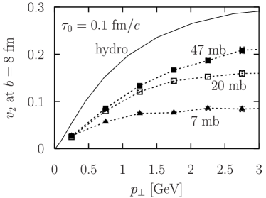
Figure 1: Comparison of the hydrodynamic result with the results obtained by a partonic transport model. Figure taken from Ref. [14].

In ideal hydrodynamics, the mean free path among particles is assumed to be zero. So the hydrodynamic prediction of $v_{2}$ should be maximum among transport theories. We naively expect that the ideal hydrodynamics corresponds to the infinite limit of the cross sections among particles in collision terms of the Boltzmann equation. In Ref. [14], Molnar and Huovinen compare $v_{2}(p_{T})$ from hydrodynamics with the one from Boltzmann equation. Special attention is paid that the same initial conditions and thermodynamic properties are used in comparison. Figure 1 shows the transverse momentum dependence of $v_{2}$ for a hydrodynamic model and a parton cascade model. $v_{2}(p_{T})$ from Boltzmann simulations is approaching to the hydrodynamic result with increasing the cross section among partons. However, even for large cross section (47 mb), the result from the Boltzmann simulation is still $\sim$ 30% smaller than the hydrodynamic result. This clearly shows the ideal hydrodynamics describes the strongly interacting matter.

1.2 Basics of Ideal Hydrodynamics

Here we concentrate our discussions on the ideal hydrodynamic model. For those who have interest in the viscous hydrodynamics, see, e.g., Ref. [15].

Hydrodynamic equations are nothing but the energy-momentum conservations $\partial_{\mu}T^{\mu\nu}=0$. In the ideal hydrodynamics, the energy-momentum tensor becomes $T^{\mu\nu}=(e+P)u^{\mu}u^{\nu}-Pg^{\mu\nu}$, where $e$ is the energy density, $P$ is the pressure, and $u^{\mu}$ is the four fluid velocity. When there are conserved quantities such as the baryon number or the number of chemically frozen hadrons, one needs to solve the continuity equations $\partial_{\mu}n_{i}^{\mu}=0$ together with the hydrodynamic equations. In order to close the system of partial differential equations, the equation of state (EoS) $P(e,n_{i})$ is needed. It is the EoS that governs the dynamics of the system in the ideal hydrodynamics. The naive applicability conditions of ideal hydrodynamics are that the mean free path among the particles is much smaller than the typical size of the system and that the system keeps local thermal equilibrium during expansion. From these conditions, one cannot use hydrodynamics for initial collisions, final free streaming and high $p_{T}$ ($\stackrel{{\scriptstyle>}}{{\sim}}$  2 GeV/$c$) particles. The quantitative criteria are more complicated in general since these come from dynamical aspects of the space-time evolution.

One usually assumes the initial hydrodynamic fields at initial (or equilibrated) time around 1 fm/$c$. One needs an interface between the pre-thermalisation stage and the hydrodynamic stage at the initial time. On the other hand, the system eventually breaks up and the assumption of the thermalisation is no longer valid at the later stage. This means a prescription of freezeout is needed in the hydrodynamic model when one evaluates the particle spectra to be observed by the detectors. Then one needs another interface between the hydrodynamic stage and the free streaming stage. In what follows, we discuss particularly equation of state, initial condition and freezeout prescription used in the literature.

1.2.1 Equation of State

The main ingredient of the hydrodynamic model is the equation of state (EoS) for thermalised matter produced in heavy ion collisions. Ideally, one uses the EoS taken from the first principle calculations of QCD, namely, lattice QCD simulations [16]. More practically, one can use the resonance gas model for the hadron phase and the massless free parton gas for the QGP phase. By matching these two EoS’s at the critical temperature, one obtains the first order phase transition model with a latent heat $\sim$1 GeV/fm³. In the mixed phase in this model, the sound velocity $c_{s}^{2}=\frac{\partial P}{\partial e}$ is vanishing. Recent lattice QCD simulations tell us that the phase transition seems to be crossover in vanishing baryonic chemical potential. Although the discontinuity of the thermodynamic variables do not exist in the crossover phase transition, it should be emphasized that the energy density and the entropy density increase more rapidly than the pressure in the vicinity of the phase transition region $\Delta T\sim 0.1T_{c}$. This also leads to very small sound velocity near the phase transition region. Therefore it is very hard to find flow observables which distinguish the crossover phase transition with a rapid change of the thermodynamic variables from the first order phase transition.

The statistical model and the blast wave model tell us that chemical freezeout temperature $T^{\mathrm{ch}}$ is larger than thermal freezeout temperature $T^{\mathrm{ch}}$ at the RHIC energies (see, e.g., discussions in Ref. [17]). Chemical freezeout temperature obtained from the statistical model analysis is very close to the (pseudo)critical temperature of the QCD phase transition. This means that the hadron phase is almost chemically frozen due to strong expansion. For chemically frozen hadronic gas, one introduces chemical potential for each hadron [18]. This modifies the chemical composition in the hadron phase compared with the chemical equilibrium hadronic gas and, consequently, changes the space-time evolution of temperature field [19].

1.2.2 Initial Condition

Once initial conditions are assigned, one can numerically simulate the space-time evolution of thermalised matter which is governed by hydrodynamic equations. Usually, initial conditions are parametrised based on some physical assumptions. Transverse profile of the energy/entropy density is assumed to be proportional to the local number of participants $\rho_{\mathrm{part}}$, the local number of binary collisions $\rho_{\mathrm{coll}}$ or linear combination of them. Initial transverse flow is usually taken to be vanishing. In either full three dimensional (3D) hydrodynamic simulations or hydrodynamic simulations of longitudinal expansion with cylindrically symmetric geometry, one needs to parametrise also longitudinal profile of initial conditions for energy density, baryon density and four fluid velocity. The initial longitudinal shape is chosen so as to reproduce the final (pseudo)rapidity distribution of hadrons. Unfortunately, the shape is not uniquely determined. Two completely different initial conditions can end up almost similar rapidity distribution. See, e.g., Ref. [20].

On the other hand, one can introduce model calculations to obtain the initial condition of hydrodynamic simulations. Event generators can be used to obtain the energy density distribution at the initial time. Recently, the SPheRIO group employs an event generator NeXus and takes an initial condition from this model in the event-by-event basis [21]. The resultant energy density distribution in the transverse plane has highly bumpy structures [21, 22]. Smooth initial conditions used in the conventional hydrodynamic simulations are no longer expected in one event. Another important example which is relevant at very high collision energies is an initial condition taken from the Colour Glass Condensate picture [23]. This will be discussed in details in Sec. 2.

1.2.3 Freezeout

Conventional prescription to obtain the invariant momentum spectra from the hydrodynamic simulations is to employ the so-called Cooper-Frye formula [24]

$$E\frac{dN_{i}}{d^{3}p}=\frac{d_{i}}{(2\pi)^{3}}\int_{\Sigma(x)}\frac{p^{\mu}d\sigma_{\mu}(x)}{\exp[(p^{\nu}u_{\nu}(x)-\mu_{i}(x))/T(x)]\pm 1}$$ (3)

where $p^{\mu}=(E,\mathbf{p})$ and $d_{i}$ are, respectively, a four momentum and the degree of freedom of a particle under consideration. Integral is performed on the freezeout hypersurface $\Sigma$. Here $d\sigma$ is an element of freezeout hypersurface on $\Sigma$. One usually assumes $\Sigma=\Sigma(T=T^{\mathrm{th}}\enskip\mathrm{or}\enskip e=e^{\mathrm{th}})$, where $T^{\mathrm{th}}$ ($e^{\mathrm{th}}$) is thermal freezeout temperature (energy density). $T^{\mathrm{th}}$ or $e^{\mathrm{th}}$ is an adjustable parameter for reproduction of the slope of $p_{T}$ spectrum. Information on the hydrodynamic simulations is taken through $d\sigma$, $u^{\mu}$, $T$ and $\mu_{i}$ at a space-time point $x$. Chemical potential for each hadron $\mu_{i}$ is not vanishing in general even in vanishing baryon density due to $T^{\mathrm{ch}}>T^{\mathrm{th}}$. Although the chemical potential is important to reproduce the particle ratios as well as the shape of the particle spectra, this is often neglected for simplicity in the literature.

The physical picture described by the Cooper-Frye formula is sometimes called “sudden freezeout” since the mean free path $\lambda$ is suddenly changed from zero to infinity through a thin freezeout hypersurface. Instead of using this, one can use a hadronic cascade model to describe the space-time evolution of hadrons [25, 26]. The mean free path among hadrons is finite and depends on hadronic species. Hence, one can describe a continuous freezeout picture through hadronic transport models. Note that continuous particle emission can be considered within the hydrodynamics [27]. Adoption of hadronic transport models after hydrodynamic evolution of the QGP liquid could refine the dynamical modeling of relativistic heavy ion collisions. However, it is not so easy to connect them in a systematic and proper way. One has to use Eq. (3) again for the boundary between the QGP liquid and the hadron gas. However, Eq. (3) describes not only out-going particles $p^{\mu}d\sigma_{\mu}>0$ but also in-coming particles $p^{\mu}d\sigma_{\mu}<0$. If one uses hydrodynamic simulations as inputs for hadronic cascade models, one must discard the in-coming particles, which violates the energy-momentum conservation. In order to remedy this problem, one need to solve hydrodynamic equations together with the appropriate kinetic equations [28].

1.3 Hydrodynamic Results for $v_{2}$

We show comparison of the hydrodynamic results with the experimental data for $v_{2}(p_{T})$, $v_{2}(\eta)$ at the RHIC energy and the excitation function of $v_{2}$.

1.3.1 $v_{2}(p_{T})$

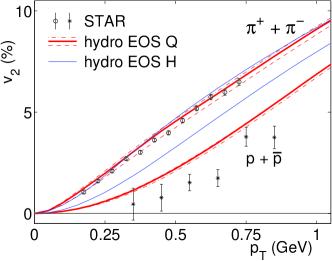
Figure 2: (left) Transverse momentum dependence of $v_{2}$ for pions and (anti)protons [8] are compared with the STAR data [30] in minimum bias Au+Au collisions at $\sqrt{s_{NN}}=130$ GeV. EoS Q stands for the equation of state with first order phase transition between the massless free parton gas and the resonance gas. On the other hand, EoS H stands for the equation of state for the resonance gas. (right) $v_{2}$ for charged hadrons as a function of pseudorapidity $\eta$ in Au+Au collisions at $\sqrt{s_{NN}}=130$ GeV [1, 32]. PCE means the EoS of partial chemical equilibrium, whereas CE means the EoS of chemical equilibrium. Figure is taken from Ref. [19].

With a help of assuming the Bjorken flow [29] for the longitudinal direction, one can solve the hydrodynamic equations only in the transverse plane at midrapidity. Systematic studies based on this (2+1)-dimensional hydrodynamic model are performed in Ref. [2]. For the EoS, complete chemical equilibrium is assumed for both the QGP phase and the hadron phase. $p_{T}$ dependences of $v_{2}$ for pions and protons from this model [8] are compared with the STAR data [30] in Fig. 2 (left). By employing the EoS with phase transition, the hydrodynamic model correctly reproduces $v_{2}(p_{T})$ and its mass-splitting behavior below $p_{T}=1$ GeV/$c$. On the other hand, $v_{2}(p_{T})$ for (anti)protons from the resonance gas model does not agree with the data. Although the reason for the difference of the result between these two EoS models is not so clear, the experimental data favors the QGP EoS. Due to the assumption of chemical equilibrium in the hadron phase, this model does not reproduce particle ratio and spectra simultaneously. It is of importance to study whether the agreement with the experimental data still holds even when the assumption of chemical equilibrium in the hadron phase is abandoned [19].

1.3.2 $v_{2}(\eta)$

One needs a full 3D hydrodynamic simulation to obtain the rapidity dependence of $v_{2}$ since either cylindrical symmetry or Bjorken flow [29] keeps us from obtaining this quantity. First analysis of $v_{2}(\eta)$ at RHIC based on the full 3D hydrodynamic model is performed in Ref. [31]. After that, the effect of early chemical freezeout on the elliptic flow is also investigated [19]. Figure 2 (right) shows $v_{2}(\eta)$ for charged hadrons in Au+Au collisions at $\sqrt{s_{NN}}=130$ GeV [1, 32]. Here the initial condition for the energy density is so chosen as to reproduce the pseudorapidity distribution of charged hadrons. Hydrodynamic results are consistent with the experimental data only near the midrapidity while hydrodynamics overpredicts the data in the forward/backward rapidity regions. Multiplicity is not so large in the forward/backward rapidity regions, so equilibration of the system tends to be spoiled.

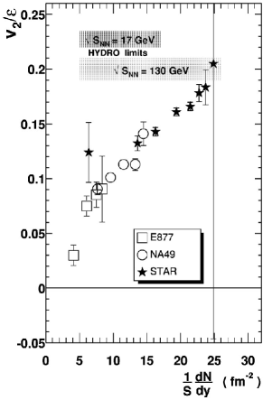
Figure 3: Excitation function of $v_{2}/\varepsilon$. Figure taken from Ref. [33].

1.3.3 Excitation function

Figure 3 shows the excitation function of $v_{2}$ compiled by the STAR Collaboration [33]. Hydrodynamic results presented in this figure are based on the same model discussed in Sec. 1.3.1. Data points continuously increase with the unit rapidity density at the AGS, SPS and RHIC energies. However, the hydrodynamic response is almost flat or slightly decreases with the multiplicity. The data points seem to reach the “hydrodynamic limit” for the first time at the RHIC energy. It will be interesting to see the same plots including the upcoming LHC results: If the system produced at LHC obeys the hydrodynamic picture, this experimental “curve” will bend at $(1/S)dN/dy\sim 25$-30.

The deviation between the hydrodynamic results and the data plots below $(1/S)dN/dy=25$ reminds us the pseudorapidity dependence of elliptic flow in Fig. 2 (right). The deviation might come from a common origin [34]: the small multiplicity both in forward rapidity region at the RHIC energy and at midrapidity at the lower collision energies could cause the partial thermalisation. In the low density limit, $v_{2}$ is actually proportional to the number density [35]. The shape of $v_{2}(\eta)$ data in forward rapidity region looks similar to that of the pseudorapidity distributions [36]. Similarly, data plots of excitation function increase almost linearly with the particle density. These results suggest that thermalisation is not achieved completely in forward rapidity region at the RHIC energy and at midrapidity at the SPS energies.

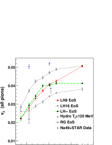
Figure 4: Excitation function from the hydro+cascade model. Figure taken from Ref. [26].

Figure 4 shows the excitation function based on the hydro+cascade model [26] with Bjorken longitudinal flow [29]. In the hadron phase, a hadronic event generator RQMD is employed in these calculations. Contrary to the conventional hydrodynamic models, freezeout processes are automatically described by this model without any adjustable parameters. The excitation function in the case of the latent heat $\sim 0.8$ GeV/fm³ linearly increases with the multiplicity, which is consistent with the experimental data. It should be noted that $v_{2}(p_{T})$, its mass dependences and particle spectra/ratio at midrapidity are also reproduced by this hybrid model [26].

1.4 Summary and Outlook

The most successful approach based on the hydrodynamic model to elliptic flow in relativistic heavy ion collisions is the hybrid one in which the QGP phase is described by the ideal hydrodynamics while the hadron phase is described by a hadronic cascade. The Bjorken scaling solution [29] is assumed in the current hydro+cascade model. This means that current hybrid models are available only near midrapidity. Therefore it is desired to develop a model in which a full 3D hydrodynamic simulation is combined with a hadronic cascade model. From agreement of excitation function between the hybrid model and the experimental data at midrapidity, the 3D hybrid model is expected to reproduce the pseudorapidity dependence of elliptic flow. It should be emphasised again that the hybrid model has its own problem on the violation of energy momentum conservations between the QGP liquid and the hadron gas. A simulation which incorporates a proper treatment at the boundary between the QGP phase and the hadron phase is now an open problem.

2 Hydrodynamic Model with a CGC Initial Condition

2.1 Toward a Unified Description of Relativistic Heavy Ion Collisions

As already discussed in the previous section, one of the important findings at RHIC is that the hydrodynamic approach to the description of elliptic flow works remarkably well when early thermalisation time and the QGP EoS are assumed [7, 8]. Hydrodynamics should work only in the situation that the mean free path $\lambda=1/\sigma\rho$ is much smaller than the typical size of the system $L$. This suggests that the particle density $\rho$ becomes very large at RHIC.

In addition to this, there are many important findings in heavy ion collisions at the RHIC energy. One of them is jet quenching [37], i.e., suppression of high $p_{T}$ hadrons in the single particle spectra and disappearance of away-side peak in the di-hadron spectra. These phenomena are not found in $dAu$ collisions [38, 39, 40, 41]: the yield of high $p_{T}$ hadrons roughly scales with the number of binary collisions $N_{\mathrm{coll}}$ and the away-side peak appears in the di-hadron spectra. So one can conclude that high $p_{T}$ partons produced in the initial hard scattering interact with the highly dense medium in the final state and that these partons lose their energies during traversing medium.

So the current RHIC data strongly suggest that the parton density created in heavy ion collisions at RHIC is dense enough to cause both large elliptic flow of bulk matter and large suppression of high-$p_{T}$ hadrons. What is an origin of this dense matter at RHIC? The bulk particle production in high energy hadronic/nuclear collisions is dominated by the small $x$ modes in the nuclear wave function, where $x$ is a momentum fraction of the incident particles. Hence, an origin of the large density could be traced to the initial parton density at small $x$ inside the ultra-relativistic nuclei before collisions. It is well known that the gluon density increases rapidly with decreasing $x$ until gluons begin to overlap in the phase space where nonlinear interaction becomes important [42]. These gluons eventually form another type of extremely dense matter, the Colour Glass Condensate (CGC) [43]. This phenomenon is characterised by a “saturation scale” $Q_{s}^{2}$ which is identified with the gluon rapidity density per unit transverse area. When $Q_{s}$ is sufficiently larger than the typical hadronic scale ($Q_{s}\gg\Lambda_{\mathrm{QCD}}$), the strong coupling constant becomes weak ($\alpha_{s}(Q_{s})\ll 1$). Moreover, the gluon occupation number in the wave function becomes huge, $\sim 1/\alpha_{s}(Q_{s})\gg 1$. Therefore the CGC can be studied by an weak coupling classical method also known as McLerran-Venugopalan (MV) model [44]. The calculations based on the CGC picture have been compared to various RHIC data. Remarkably, the CGC results on the global observables, e.g., the centrality, rapidity and energy dependences of charged hadron multiplicities agree with the RHIC data under the assumption of parton-hadron duality [45].

In relativistic heavy ion collisions, the CGC could be a seed of the QGP [46]. So hydrodynamic initial conditions can be calculated from the two CGC collisions. One needs a non-equilibrium model which describes equilibration from the produced gluon distribution to a local thermal distribution. This is, however, beyond the present work. In this work, the rapidity, transverse position and centrality dependences of the number of produced gluons are identified with the hydrodynamic initial condition of a thermalised QGP.

Some of the problems which are inherent in a particular approach can be removed. For instance, one conventionally parametrises initial conditions in the hydrodynamic simulations shortly after a collision of two nuclei by hand. Therefore it is desired to take an initial condition which is obtained by a reliable theory. On the other hand, most of the calculations based on the CGC do not include final state interactions. According to estimation of initial parton productions from a classical lattice Yang-Mills simulation based on the CGC [47, 48], the transverse energy per particle is roughly $E_{T}/N\sim 1.5$ GeV, while the experimental data yields $E_{T}/N\sim 0.6$ GeV [49]. Moreover, elliptic flow from a classical Yang-Mills simulation is inconsistent with RHIC data [50]. Those discrepancies, which are mainly due to the lack of collective effects, will be removed by introducing further time evolution through, e.g., hydrodynamics. For the calculation of parton energy loss, one needs time evolution of parton density. Bjorken expansion [29] is assumed for the evolution of parton density in almost all work except Refs. [51, 52].

We have already developed a unified model (CGC+Hydro+Jet model) in which hydrodynamic evolution, CGC initial conditions, and the production and propagation of high $p_{T}$ partons are combined [23]. Only the soft sector, i.e., the production of gluons in CGC collisions and the hydrodynamic afterburner for the CGC initial condition is discussed in this paper. For further details of the model and the results for high $p_{T}$ regions such as centrality dependences of the nuclear modification factors and the azimuthal correlation functions, see Ref. [23].

2.2 Gluon Production from a CGC picture

We employ the $k_{T}$ factorisation formula for the production of gluons from CGC collisions along the line of work by Kharzeev, Levin and Nardi (KLN) [45]. The number of produced gluons in the $k_{T}$-factorisation formula is given by [42, 53, 54, 55]

$$\frac{dN_{g}}{d^{2}x_{\perp}dy} = \frac{4\pi^{2}N_{c}}{N_{c}^{2}-1}\int\frac{d^{2}p_{T}}{p^{2}_{T}}\int d^{2}k_{T}\alpha_{s}(Q^{2})$$ (4)

$$\times \phi_{A}(x_{1},k_{T}^{2};\mathbf{x}_{\perp})\phi_{B}(x_{2},(p_{T}-k_{T})^{2};\mathbf{x}_{\perp}),$$

where $x_{1,2}=p_{T}\exp(\pm y)/\sqrt{s}$, and $y$ and $p_{T}$ are a rapidity and a transverse momentum of a produced gluon. Running coupling constant $\alpha_{s}$ is evaluated at the scale $Q^{2}=\max(k^{2}_{T},(p_{T}-k_{T})^{2})$. The unintegrated gluon distribution $\phi$ is related to the gluon density of a nucleus by

$$xG_{A}(x,Q^{2})=\int^{Q^{2}}d^{2}k_{T}d^{2}x_{\perp}\phi_{A}(x,k^{2}_{T};\mathbf{x}_{\perp}).$$ (5)

Motivated by the KLN approach, we use a simplified assumption about the unintegrated gluon distribution function:

$$\phi_{A}(x,k^{2}_{T};\mathbf{x}_{\perp})\,\,=\left\{\begin{array}[]{l}\frac{\kappa C_{F}}{2\pi^{3}\alpha_{s}(Q^{2}_{s})}\frac{Q_{s}^{2}}{Q_{s}^{2}+\Lambda^{2}},\,\quad k_{T}\,\leq\,Q_{s},\\ \frac{\kappa C_{F}}{2\pi^{3}\alpha_{s}(Q^{2}_{s})}\,\frac{Q^{2}_{s}}{k^{2}_{T}+\Lambda^{2}},\quad k_{T}\,>\,Q_{s},\end{array}\right.$$ (6)

where $C_{F}=(N_{c}^{2}-1)/(2N_{c})$. We introduce a small regulator $\Lambda=0.2$ GeV/$c$ in order to have a smooth distribution in the forward rapidity region $|y|>4.5$ at RHIC. Other regions are not affected by introducing a small regulator. The above distribution depends on the transverse coordinate $\mathbf{x}_{\perp}$ through $Q_{s}^{2}$. Saturation momentum of a nucleus $A$ in $A+B$ collisions is obtained by solving the following implicit equation with respect to $Q_{s}$ at fixed $x$ and $\mathbf{x}_{\perp}$

$$Q^{2}_{s}(x,\mathbf{x}_{\perp})=\frac{2\pi^{2}}{C_{F}}\alpha_{s}(Q^{2}_{s})xG(x,Q^{2}_{s})\rho^{A}_{\mathrm{part}}(\mathbf{x}_{\perp}),$$ (7)

where

$$\rho^{A}_{\mathrm{part}}(\mathbf{x}_{\perp})=T_{A}(\mathbf{x}_{\perp})\left\{1-[1-\sigma^{\mathrm{in}}_{NN}T_{B}(\mathbf{x}_{\perp})/B]^{B}\right\}.$$ (8)

The number of participants is given by

$$N_{\mathrm{part}}=\int d^{2}x_{\perp}(\rho^{A}_{\mathrm{part}}(\mathbf{x}_{\perp})+\rho^{B}_{\mathrm{part}}(\mathbf{x}_{\perp})).$$ (9)

We take a simple perturbative form for the gluon distribution in a nucleon

$$xG(x,Q^{2})=K\ln\left(\frac{Q^{2}+\Lambda^{2}}{\Lambda_{\mathrm{QCD}}^{2}}\right)x^{-\lambda}(1-x)^{n}$$ (10)

where $\Lambda=\Lambda_{\mathrm{QCD}}=0.2$ GeV. $K$ is used to control saturation scale in Eq. (7) [56]. We choose $K=0.7$ for $\lambda=0.2$ so that the average saturation momentum in the transverse plane yields $\langle Q_{s}^{2}(x=0.01)\rangle\sim 2.0$ GeV${}^{2}/c^{2}$ in Au+Au collisions at impact parameter $b=0$ at RHIC. Similar to the KLN approach, $x^{-\lambda}$ dependence of the saturation scale is motivated by the Golec-Biernat–Wüsthoff model [57]. The factor $(1-x)^{n}$ shows that gluon density becomes small at $x\to 1$. $n$ usually depends on the scale $Q^{2}$. Here we take $n=4$ as in the KLN approach [45].

We obtain the rapidity distribution for produced gluons at each transverse point $\mathbf{x}_{\perp}$ by performing the integral of Eq. (4) numerically. The transverse energy distribution $dE_{T}/dy$ is also obtained by weighting the transverse momentum of gluons $p_{T}$ in the integration with respect to $p_{T}$ in Eq. (4). We cut off the integral range of $p_{T}$ in Eq. (4) since only the low $p_{T}$ partons are assumed to reach the local thermal equilibrium. We set the cut-off momentum as $p_{T,\mathrm{cut}}=3$ GeV/$c$ which corresponds roughly to the maximum saturation scale at $x=0.01$ at the origin $\mathbf{x}_{\perp}=\mathbf{0}$ in central Au+Au collisions at RHIC.

In order to obtain initial conditions for hydrodynamics, one needs a non-equilibrium description for the collisions of heavy nuclei. Leaving this problem for the future work, we assume that the system of gluons initially produced from the CGC reaches a kinematically and chemically equilibrated state at a short time scale.

There are two ways to provide initial conditions from the CGC, i.e., matching of number density (IC-$n$) and matching of energy density (IC-$e$). Here, we employ the former prescription, i.e., IC-$n$. For the result from IC-$e$, see Ref. [23]. Assuming Bjorken’s ansatz $y=\eta_{\mathrm{s}}$ [29] where $\eta_{\mathrm{s}}$ is the space-time rapidity $\eta_{\mathrm{s}}=(1/2)\ln(x^{+}/x^{-})$, we obtain the number density for gluons at a space-time point $(\tau_{0},\mathbf{x}_{\perp},\eta_{\mathrm{s}})\equiv(\tau_{0},\vec{x})$ from Eq. (4)

$$n_{g}(\tau_{0},\vec{x})=\frac{dN_{g}}{\tau_{0}d\eta_{\mathrm{s}}d^{2}x_{\perp}}.$$ (11)

Number density $n$ for the massless free parton system can be written:

$$n = \left(\frac{3}{4}d_{q}+d_{g}\right)\frac{\zeta(3)}{\pi^{2}}T^{3},$$ (12)

where $d_{q}=2N_{c}N_{s}N_{f}=36$, $d_{g}=2(N_{c}^{2}-1)=16$ and $\zeta(3)=1.20206$. Thus, we obtain the initial temperature field in the three-dimensional (3D) space from the number density (IC-$n$):

$$T(\tau_{0},\vec{x})=\left\{\frac{\pi^{2}n(\tau_{0},\vec{x})}{43\zeta(3)}\right\}^{1/3}.$$ (13)

When the temperature at ($\tau_{0}$, $\vec{x}$) is below the critical temperature $T_{\mathrm{c}}=170$ MeV, the all thermodynamic variables in the cell are set to zero.

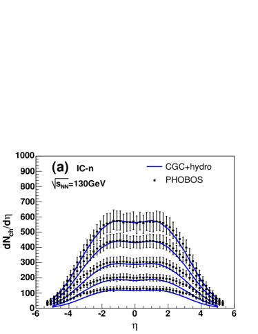
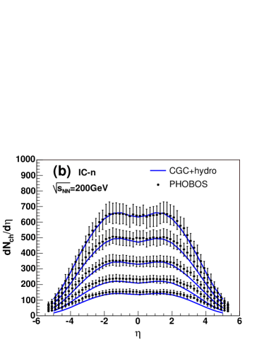
Figure 5: Pseudorapidity distributions of charged hadrons in Au + Au collisions at $\sqrt{s_{NN}}$= (a) 130 and (b) 200 GeV are compared to the PHOBOS data [58]. Figure taken from Ref. [23]

2.3 Results

In Fig. 5, pseudorapidity distributions of charged hadrons in Au + Au collisions at both $\sqrt{s_{NN}}=130$ and 200 GeV are compared with the PHOBOS data [58]. Impact parameters in each panel are, from top to bottom, 2.4, 4.5, 6.3, 7.9, and 9.1 fm (2.5, 4.4, 6.4, 7.9, and 9.1 fm) for $\sqrt{s_{NN}}=$ 200 (130) GeV. These impact parameters are evaluated from the average number of participants at each centrality estimated by PHOBOS [58]. It should be also emphasized that it is not easy to parametrize such initial conditions which reproduce the data with the same quality as the CGC initial conditions presented here.

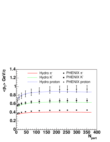
Figure 6: Mean transverse momenta for pions, kaons and protons as a function of $N_{\mathrm{part}}$ [59]. Here contribution only from hydrodynamic components is taken into account. $T^{\mathrm{th}}=100$ MeV is used for all centralities. Figure taken from Ref. [23]

Mean transverse momenta $\langle p_{T}\rangle$ for pions, kaons and protons as a function of $N_{\mathrm{part}}$ are compared with the PHENIX data [59] in Fig. 6. Although our results are slightly smaller than the data in central and semicentral regions, the overall trend is consistent with the data. For pions, the semihard spectrum starts to be comparable with the soft spectrum around $p_{T}=1.5$-2.0 GeV/$c$. We reproduce the $p_{T}$ spectra for pions by including contribution from quenched jets. So the deviation for pions can be filled by the semihard spectrum. While semihard components for kaons and protons are very small in low and intermediate $p_{T}$ regions. A little more radial flow is needed to gain the mean transverse momentum in central collisions.

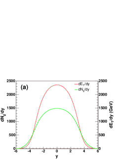
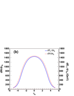
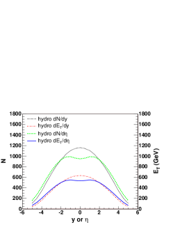
Figure 7: (Pseudo)rapidity distribution of (a) gluons produced from CGC collisions, (b) partons at initial time, and (c) final total hadrons in Au + Au collisions at $\sqrt{s_{NN}}=$ 200 GeV.

Both the KLN approach and the hydrodynamic model with a CGC initial condition reproduce the centrality and rapidity dependences of particle distributions. Then, what is the role of hydrodynamic evolution in comparison with the KLN approach? The main difference between these two approaches is whether final state interactions are taken into account. The initial transverse energy per particle is estimated to be $E_{T}/N_{g}\sim 1.6$ GeV at $y=0$. It becomes $E_{T}/N_{g}=1.0$ GeV after assuming a thermal state. The effect of the hydrodynamic afterburner is to reduce the transverse energy per particle due to $pdV$ work. We find that $(dE_{T}/dy)/(dN/dy)|_{y=0}=0.54$ GeV and $(dE_{T}/d\eta)/(dN/d\eta)|_{\eta=0}=0.56$ GeV.

2.4 Summary and Outlook

Our approach is a first step toward a unified dynamical modeling of relativistic heavy ion collisions.

The main goal has been developing a consistent dynamical framework for the space-time evolution of both bulk matter and hard jets. In order to accomplish this, much remains are to be done.

• More sophisticated wave function should be used to calculate the production of initial gluons. At midrapidity, results from the classical Yang-Mills equation can be used. In forward rapidity region at the RHIC energy or even at midrapidity at the LHC energy, one needs a quantum evolution.

• As discussed in the Sec. 1, the hadron phase should be described by a hadronic transport model. This will improve $v_{2}$ in forward rapidity regions in the hydrodynamic result.

• EoS from the recent lattice QCD simulations should be used in the hydrodynamic simulations.

• Chemical non-equilibrium process will be taken into account by solving the rate equation for the number of quarks and gluons together with the hydrodynamic equations [60]. The amount of energy loss of partons depends on a species of both probe parton and medium parton. So the correct chemical composition in the QGP phase will lead to reproduction of nuclear modification factors without any free parameters.

Reference

References

- [1] Ackermann K H et al(STAR Collaboration) 2001 Phys. Rev. Lett.86 402
- [2] Kolb P F, Huovinen P, Heinz U and Heiselberg H 2001 Phys. Lett.B 500 232 Huovinen P, Kolb P F, Heinz U W, Ruuskanen P V and Voloshin S A 2001 Phys. Lett.B 503 58 Kolb P F, Heinz U W, Huovinen P, Eskola K J and Tuominen K 2001 Nucl. Phys.A696 197
- [3] Alt C et al(NA49 Collaboration) 2003 Phys. Rev.C 68 034903 Agakichiev G et al(CERES/NA45 Collaboration) 2004 Phys. Rev. Lett.92 032301
- [4] Shuryak E 2004 J. Phys. G: Nucl. Part. Phys.30 S1221 Teaney D 2003 Phys. Rev.C 68 034913
- [5] Bleicher M and Stocker H 2002 Phys. Lett.B 526 309
- [6] Retière F 2004 J. Phys. G: Nucl. Part. Phys.30 S827
- [7] Huovinen P 2003 Preprint nucl-th/0305064
- [8] Kolb P F and Heinz U 2003 Preprint nucl-th/0305084
- [9] Ollitrault J Y 1992 Phys. Rev.D 46 229 Ollitrault J Y 1998 Nucl. Phys.A 638 195
- [10] Poskanzer A M and Voloshin S A 1998 Phys. Rev.C 58 1671
- [11] Kolb P 2003 Phys. Rev.C 68 031902
- [12] Adams J et al(STAR Collaboration) 2004 Phys. Rev. Lett.92 062301
- [13] Kolb P F, Sollfrank J and Heinz U W 2000 Phys. Rev.C 62 054909
- [14] Molnar D and Huovinen P 2004 Preprint nucl-th/0404065
- [15] Muronga A 2004 Phys. Rev.C 69 034903 Muronga A and Rischke D H 2004 preprint nucl-th/0407114
- [16] Karsch F 2002 Lect. Notes Phys. 583 209
- [17] Shuryak E V 1999 Nucl. Phys.A 661 119 Heinz U 1999 Nucl. Phys.A 661 140
- [18] Bebie H, Gerber P, Goity J L and Leutwyler H 1992 Nucl. Phys.B 378 95
- [19] Hirano T and Tsuda K 2002 Phys. Rev.C 66 054905
- [20] Huovinen P, Ruuskanen P V and Sollfrank J 1999 Nucl. Phys.A 650 227
- [21] Osada T, Aguiar C E, Hama Y and Kodama T 2001 Preprint nucl-th/0102011 Hama Y, Kodama T and Socolowski Jr O 2004 hep-ph/0407264
- [22] Gyulassy M, Rischke D H and Zhang B 1997 Nucl. Phys.A613 397
- [23] Hirano T and Nara Y 2004 Nucl. Phys.A (in press)
- [24] Cooper F and Frye G 1974 Phys. Rev.D 10 186
- [25] Bass S A and Dumitru A 2000 Phys. Rev.C 61 064909
- [26] Teaney D, Lauret J and Shuryak E V 2001 Preprint nucl-th/0110037
- [27] Grassi F, Hama Y and Kodama T 1995 Phys. Lett.B 355 9 Socolowski O J, Grassi F, Hama Y and Kodama T 2004 Preprint hep-ph/0405181
- [28] Bugaev K A 2003 Phys. Rev. Lett.90 252301 Bugaev K A 2004 Preprint nucl-th/0401060
- [29] Bjorken J D 1983 Phys. Rev.D 27 140
- [30] Adler C et al(STAR Collaboration) 2001 Phys. Rev. Lett.87 182301
- [31] Hirano T 2001 Phys. Rev.C 65 011901
- [32] Back B B et al(PHOBOS Collaboration) 2002 Phys. Rev. Lett.89 222301
- [33] Adler C et al(STAR Collaboration) 2002 Phys. Rev.C 66 034904
- [34] Heinz U and Kolb P 2004 J. Phys. G: Nucl. Part. Phys.30 S1229
- [35] Heiselberg H and Levy A M 1999 Phys. Rev.C 59 2716
- [36] Steinberg P A 2002 Nucl. Phys.A 698 314c
- [37] Gyulassy M, Vitev I, Wang X N and Zhang B W 2003 Preprint nucl-th/0302077 Kovner A and Wiedemann U A 2003 Preprint hep-ph/0304151
- [38] Back B B et al(PHOBOS Collaboration) 2003 Phys. Rev. Lett.91 072302
- [39] Adler S S et al(PHENIX Collaboration) 2003 Phys. Rev. Lett.91 072303
- [40] Adams J et al(STAR Collaboration) 2003 Phys. Rev. Lett.91 072304
- [41] Arsene I et al(BRAHMS Collaboration) 2003 Phys. Rev. Lett.91 072305
- [42] Gribov L V, Levin E M and Ryskin M G 1983 Phys. Rept. 100 1
- [43] Iancu E and Venugopalan R 2003 Preprint hep-ph/0303204
- [44] McLerran L D and Venugopalan R 1994 Phys. Rev.D 49 2233 McLerran L D and Venugopalan R 1994 Phys. Rev.D 49 3352 McLerran L D and Venugopalan R 1994 Phys. Rev.D 50 2225
- [45] Kharzeev D and Nardi M 2001 Phys. Lett.B 507 121 Kharzeev D and Levin E 2001 Phys. Lett.B 523 79 Kharzeev D, Levin E and Nardi M 2001 Preprint hep-ph/0111315 Kharzeev D, Levin E and Nardi M 2004 Nucl. Phys.A 730 448
- [46] Gyulassy M and McLerran L 2004 Preprint nucl-th/0405013
- [47] Krasnitz A, Nara Y and Venugopalan R 2003 Nucl. Phys.A 727 427
- [48] Lappi T 2003 Phys. Rev.C 67 054903
- [49] Bazilevsky A et al(PHENIX Collaboration) 2003 Nucl. Phys.A 715 486c
- [50] Krasnitz A, Nara Y and Venugopalan R 2003 Phys. Lett.B 554 21
- [51] Gyulassy M, Vitev I, Wang X N and Huovinen P 2002 Phys. Lett.B 526 301
- [52] Hirano T and Nara Y 2002 Phys. Rev.C 66 041901 Hirano T and Nara Y 2003 Phys. Rev. Lett.91 082301 Hirano T and Nara Y 2003 Phys. Rev.C 68 064902 Hirano T and Nara Y 2004 Phys. Rev.C 69 034908
- [53] Gribov L V, Levin E M and Ryskin M G 1981 Phys. Lett.B 100 173
- [54] Laenen E and Levin E 1994 Ann. Rev. Nucl. Part. Sci. 44 199
- [55] Szczurek A 2003 Acta Phys. Polon. B 34 3191
- [56] Baier R, Kovner A and Wiedemann U A 2003 Phys. Rev.D 68 054009
- [57] Golec-Biernat K and Wusthoff M 1999 Phys. Rev.D 59 014017 Golec-Biernat K and Wusthoff M 1999 Phys. Rev.D 60 114023
- [58] Back B B et al2003 Phys. Rev. Lett.91 052303
- [59] Adler S S et al(PHENIX Collaboration) 2003 Preprint nucl-ex/0307022
- [60] Biro T S, van Doorn E, Muller B, Thoma M H and Wang X N 1993 Phys. Rev.C 48 1275 Srivastava D K, Mustafa M G and Muller B 1997 Phys. Rev.C 56 1064 Elliott D M and Rischke D H 2000 Nucl. Phys.A671 583