Quark Propagation in the Presence of a $<A_{\mu}^{a}A_{a}^{\mu}>$ Condensate

Abstract

There is a good deal of current interest in the condensate $<g^{2}A_{\mu}^{a}A_{a}^{\mu}>$ which has recently be shown to be the Landau gauge version of a more general gauge-invariant expression. In the present work we consider quark propagation in the presence of such a condensate which we assume to be present in the vacuum. We describe the vacuum as a random medium of gluon fields. We discuss quark propagation in that medium and show that the quark propagator has no on-mass-shell pole indicating that a quark cannot propagate over extended distances. That is, the quark is a nonpropagating mode in the gluon condensate.

I Introduction

Some years ago we presented a discussion of the properties of the gluon condensate [1,2]. Central to our work was the specification of the condensate $<g^{2}A^{2}>$ which was obtained from the known value of $<0\mid(\alpha_{s}/\pi)G_{a}^{\mu\gamma}G^{a}_{\mu\gamma}\mid 0>$. (The value of the latter quantity was the only parameter we needed for our analysis.) We obtained a dynamical gluon mass of $m_{G}$=649 MeV and a dynamical quark mass of $m_{q}^{Gl}$=432 MeV, which arose from coupling to the gluon condensate [1,2]. In addition, we predicted a glueball mass of $1.0\pm 0.15$ GeV.

Our work was limited by the fact that the condensate $<g^{2}A^{2}>$ was thought to be non gauge invariant. However, recent years have shown a renewed interest in such a condensate. For example, we note that the operator $G_{\mu\nu}^{a}G_{a}^{\mu\nu}$ generates terms of order $1/p^{4}$ in the operator product expansion, while $A_{\mu}A^{\mu}$ is the only term that has a vacuum expectation value which will generate $1/p^{2}$ terms in studies making use of the operator product expansion. There is significant empirical evidence for the importance of such $1/p^{2}$ terms [3].

The issue of gauge invariance has been discussed by several authors [4,5] and it was argued that $<A^{2}_{\mu}>$ may be important for the study of the topological structure of the vacuum and quark confinement [4,6,7]. Kondo [4] was responsible for introducing a BRST-invariant condensate of dimension 2

$$\mathcal{O}=\frac{1}{\Omega}<\int d^{4}x\,\mbox{Tr}\left(\frac{1}{2}A_{\mu}(x)\cdot A_{\mu}(x)-\alpha i\,c(x)\cdot\bar{c}(x)\right)>$$ (1.1)

where $c(x)$ are Faddeev-Popov ghosts, $\alpha$ is the gauge-fixing parameter and $\Omega$ is the integration volume. To quote Kondo: “It is clear that $\mathcal{O}$ reduces to $A^{2}_{min}$ in the Landau gauge $\alpha=0$. Therefore, the Landau gauge turns out to be a rather special case in which we do not need to consider the ghost condensation.” Here, the minimum value of the integrated squared potential is $A^{2}_{min}$, which has a definite physical meaning [4].

Recently Arriola, Bowman and Broniowski [8] have made use of lattice data for the quark propagator. They have considered an operator product expansion (OPE) in the analysis of the QCD lattice data, including $<A^{2}>/Q^{2}$ terms and use the relation $m_{G}^{2}=(3/32)g^{2}<A^{2}>$ to obtain $m_{G}=(625\pm 33)$ MeV, a numerical result that is consistent with the one we have obtained by a different method [1,2].

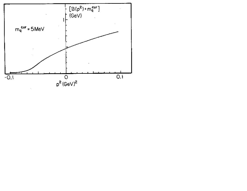
Figure 3: The mass parameter $[B(p^{2})+m_{q}^{cur}]$ for up and down quarks with $m_{q}^{cur}$ =5 MeV.

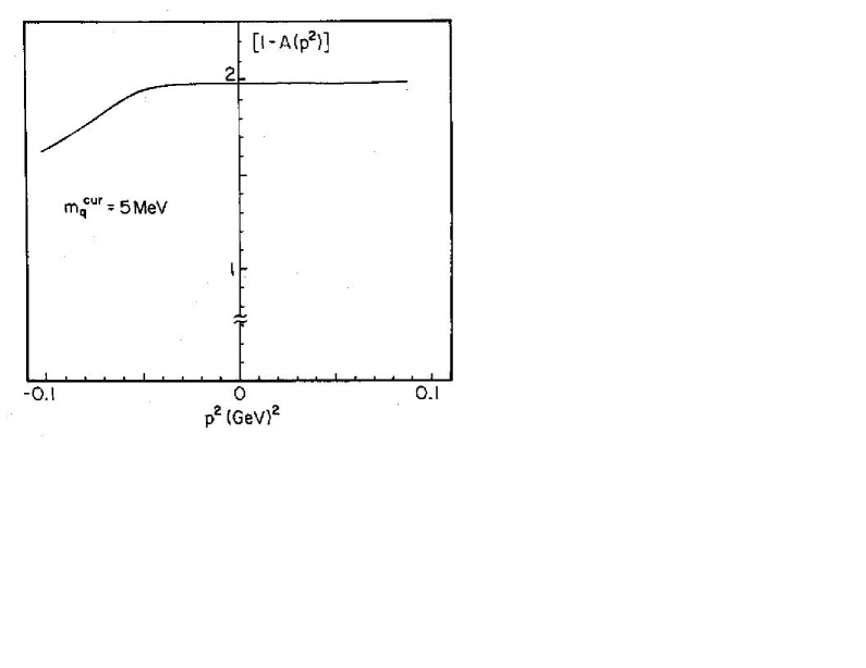
Figure 4: The wave function renormalization parameter $[1-A(p^{2})]$ for up and down quarks.

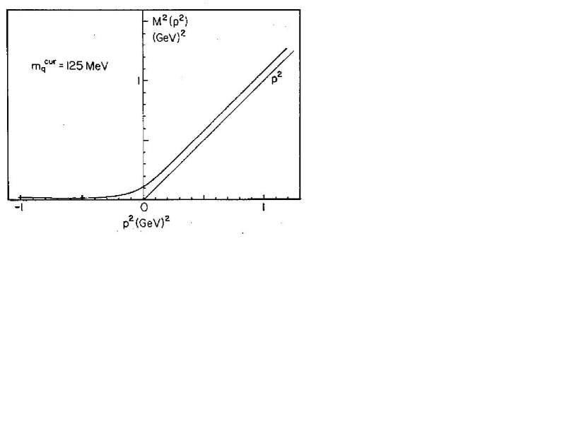
Figure 5: The square of the dynamical mass, $M^{2}(p^{2})$, for the strange quark. Here $m_{q}^{cur}$=125 MeV. (Note the change in scale with respect to Figs. 2-4.)

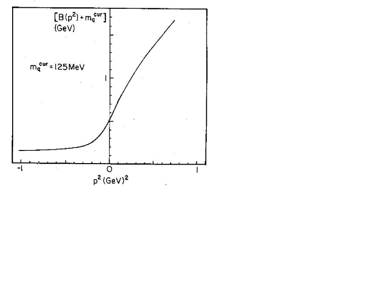
Figure 6: The mass parameter $[B(p^{2})+m_{q}^{cur}]$ for the strange quark. (Here $m_{q}^{cur}$ = 125 MeV.)

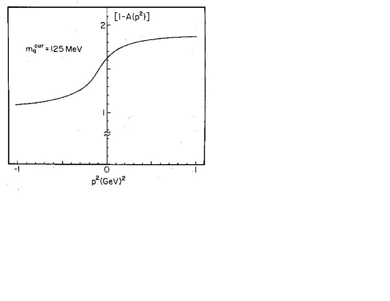
Figure 7: The wave function renormalization parameter $[1-A(p^{2})]$ for the strange quark. [See caption to Fig. 5.]

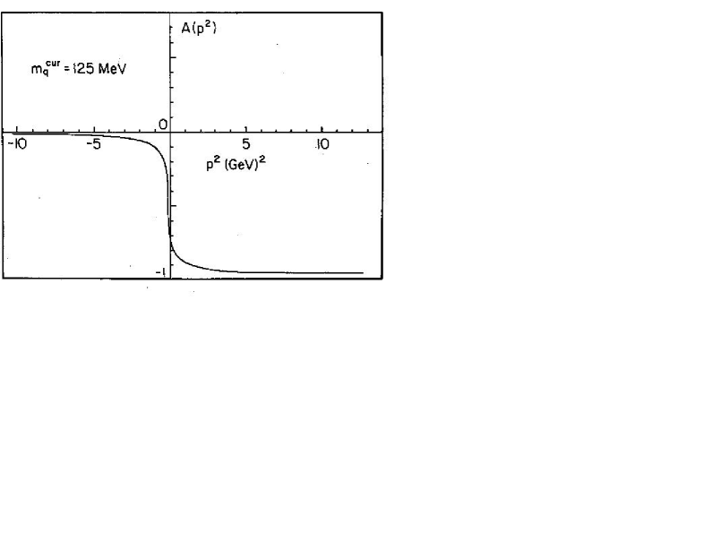
Figure 8: The function $A(p^{2})$ for the strange quark $(m_{q}^{cur}$=125 MeV) for an extended range of values of $p^{2}$.

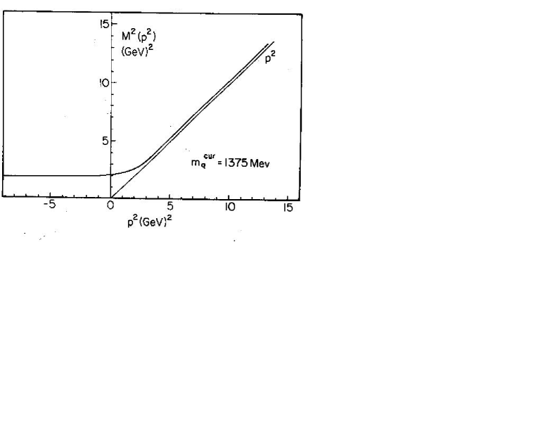
Figure 9: The square of the dynamical mass, $M^{2}(p^{2})$, for the charm quark. Here $m_{q}^{cur}$ = 1375 GeV. (Note the change of scale with respect to Figs. 2-8.)

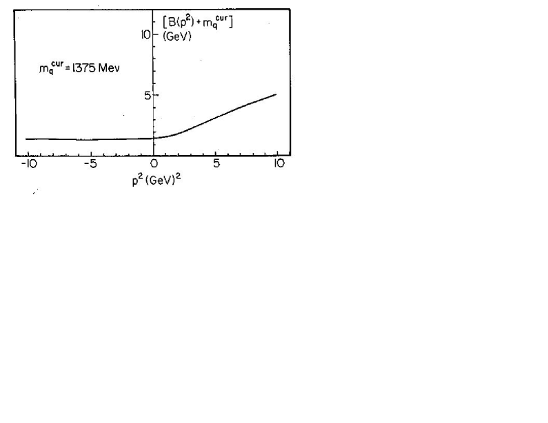
Figure 10: The mass parameter $[B(p^{2})+m_{q}^{cur}]$ for the charm quark. (Here $m_{q}^{cur}$ = 1375 MeV.) [See caption to Fig. 9.]

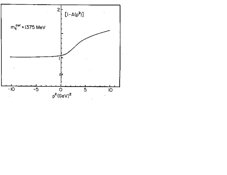
Figure 11: The wave function renormalization parameter, $[1-A(p^{2})]$ for the charm quark. Here $m_{q}^{cur}$ = 1375 GeV. (Note the change of scale with respect to Figs. 2-8.)

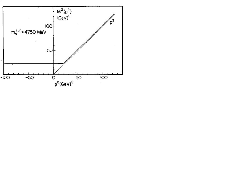
Figure 12: The square of the dynamical mass, $M^{2}(p^{2})$, for the bottom quark. Here $m_{q}^{cur}$ = 4750 MeV. (Note the change of scale with respect to Figs. 2-11.)

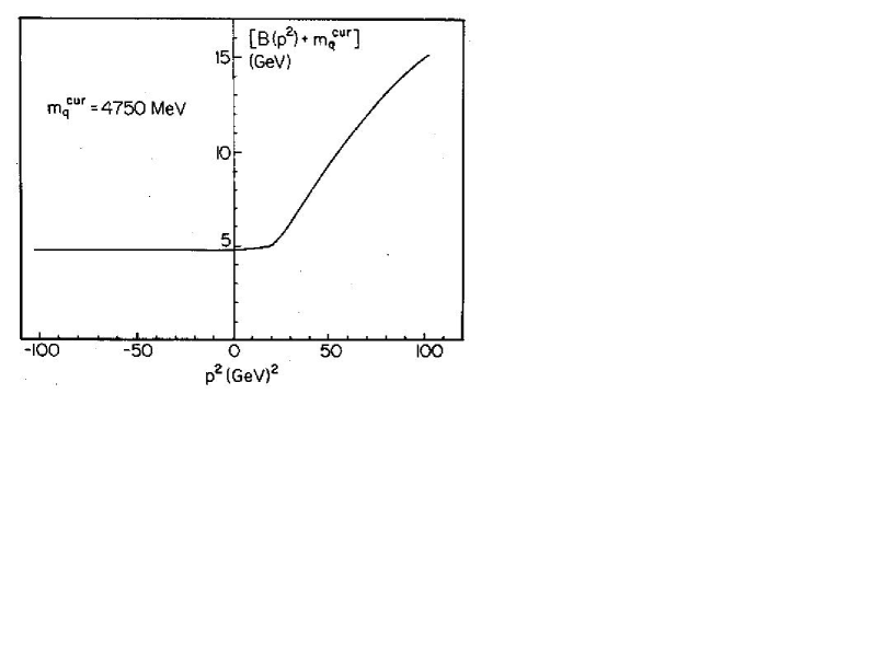
Figure 13: The mass parameter $[B(p^{2})+m_{q}^{cur}]$ for the bottom quark. Here $m_{q}^{cur}$ = 4750 MeV. [See caption to Fig. 12.]

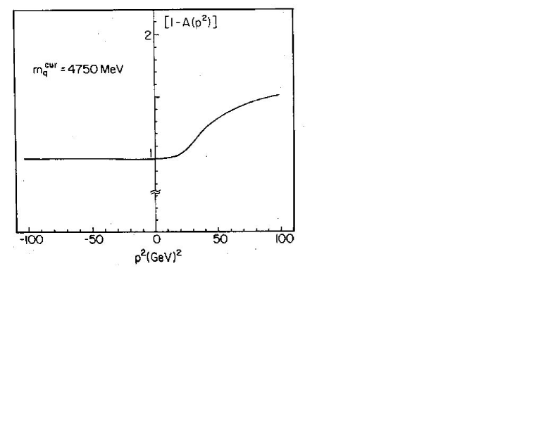
Figure 14: The wave function renormalization parameter $[1-A(p^{2})]$ for the bottom quark. Here $m_{q}^{cur}$ = 4750 MeV. [See caption to Fig. 12.]

Our work contains the following material. In Section II we will introduce a description of the QCD vacuum as a random medium and define our model for the matrix elements of the condensate field. In Section III we review the theory of wave propagation in a random medium and introduce the quark propagator. In Section IV we calculate the quark self-energy, $\Sigma(p)=A(p^{2})\hbox to0.0pt{\hbox to5.03125pt{\hfil/\hfil}\hss}p+B(p^{2})$, and present results for $M(p^{2})=(B(p^{2})+m_{q}^{cur})/(1-A(p^{2}))$, $B(p^{2})+m_{q}^{cur}$ and $[1-A(p^{2})]$ in Figs. 2-14. Section V contains some further discussion and conclusions.

II The QCD Vacuum as a Random Medium

We now proceed to consider quark propagation in a random medium which is characterized, in part, by finite value of the $<A^{2}>$ condensate. It is useful to separate the vector potential into a condensate field and a fluctuating field. We write

$$A_{i}^{a}(x)=\mathbb{A}^{a}_{i}(x)+\mathcal{A}_{i}^{a}(x).$$ (2.1)

This division of the vector potential into a condensate field, which we assume may be treated as a classical random field, and a fluctuation field, $\mathcal{A}_{\mu}^{a}(x)$, will be useful. The basic idea is that, independent of the nature of the condensate, be it a monopole vortex or instanton condensate, there is a natural separation of the field into a nonperturbative condensate field and a fluctuation field which can be treated perturbatively. (Some discussion of this separation is given in Shuryak’s book with reference to its use in a QCD sum-rule analysis [9].)

We introduce a vacuum state which has the following properties:

$$<vac\mid\mathbb{A}_{a}^{i}(0)\mid vac>=0,$$ (2.2)

$$<vac\mid\mathbb{A}_{a}^{i}(0)\mathbb{A}_{b}^{j}(0)\mid vac>=\frac{\delta_{ij}}{3}\phi_{0}^{2}\frac{\delta_{ab}}{8},$$ (2.3)

etc.

We will find it useful to generalize this result to provide a covariant description of the vacuum state. We define a vacuum state, $\widetilde{\mid vac>}$, which has the following properties

$$<\widetilde{vac}\mid\mathbb{A}_{\mu}^{a}(0)\mid\widetilde{vac}>=0,$$ (2.4)

$$<\widetilde{vac}\mid g^{2}\mathbb{A}_{\mu}^{a}(0)\mathbb{A}^{b}_{\nu}(0)\mid\widetilde{vac}>=-\frac{g_{\mu\nu}}{4}g^{2}\phi_{0}^{2}\frac{\delta_{ab}}{8},$$ (2.5)

$$<\widetilde{vac}\mid\mathbb{A}_{\mu}^{a}(0)\mathbb{A}_{\nu}^{b}(0)\mathbb{A}^{c}_{\rho}(0)\mid\widetilde{vac}>=0,$$ (2.6)

$$<\widetilde{vac}\mid g^{4}\mathbb{A}_{\mu}^{a}(0)\mathbb{A}_{\nu}^{b}(0)\mathbb{A}^{c}_{\rho}(0)\mathbb{A}^{d}_{\eta}(0)\mid\widetilde{vac}>\,\,\,\,\,\,\,\,\,\,\,\,\,\,\,\,\,\,\,\,\,\,\,\,\,\,\,\,\,\,\,\,\,\,\,\,\,\,\,\,\,$$ (2.7)

$$=\,<\widetilde{vac}\mid\mathbb{A}_{\mu}^{a}(0)\mathbb{A}^{b}_{\nu}(0)\mid\widetilde{vac}><\widetilde{vac}\mid\mathbb{A}_{\rho}^{c}(0)\mathbb{A}^{d}_{\eta}(0)\mid\widetilde{vac}>$$

$$+<\widetilde{vac}\mid\mathbb{A}_{\mu}^{a}(0)\mathbb{A}^{c}_{\rho}(0)\mid\widetilde{vac}><\widetilde{vac}\mid\mathbb{A}_{\nu}^{b}(0)\mathbb{A}^{d}_{\eta}(0)\mid\widetilde{vac}>$$

$$+<\widetilde{vac}\mid\mathbb{A}_{\mu}^{a}(0)\mathbb{A}^{d}_{\eta}(0)\mid\widetilde{vac}><\widetilde{vac}\mid\mathbb{A}_{\nu}^{b}(0)\mathbb{A}^{c}_{\rho}(0)\mid\widetilde{vac}>$$

$$=(g_{\mu\nu}g_{\rho\eta}\delta_{ab}\delta_{cd}+g_{\mu\rho}g_{\nu\eta}\delta_{ac}\delta_{bd}+g_{\mu\eta}g_{\nu\rho}\delta_{ad}\delta_{bc})g^{4}\phi_{0}^{4}/(16\cdot 64),$$ (2.8)

etc. Here, all odd correlation functions are taken to be zero and all even correlation functions may be expressed in terms of the two-point correlation function, as in Eq. (2.8). This characterization is that of a Gaussian random medium.

More generally, we might put

$$<\widetilde{vac}\mid g^{2}\mathbb{A}_{\mu}^{a}(x)\mathbb{A}^{b}_{\nu}(y)\mid\widetilde{vac}>=-\frac{g_{\mu\nu}}{4}g^{2}\phi_{0}^{2}\frac{\delta_{ab}}{8}\exp\left[-\mid(x-y)^{2}\mid^{1/2}/L\right]$$ (2.9)

where $L$ is a correlation length. The model we will study has $L\rightarrow\infty$. That is, $L$ will be taken to be large compared to the characteristic mean-free-path associated with the damping of the quark propagator.

We wish to study the equation for the quark field

$$(i\gamma^{\mu}\partial_{\mu}-g\mathbb{A}^{\mu}_{a}(x)\gamma_{\mu}\frac{\lambda^{a}}{2})\psi(x)=0$$ (2.10)

and the associated quark propagator. We have only included the condensate field in Eq. (2.10) and will treat $\mathbb{A}_{\mu}^{a}(x)$ as a random field having the properties described above. With that goal in mind, we will review the classical theory of wave propagation in random media.

III Wave Propagation in a Random Medium

A useful review of wave propagation in random media has been given by Frisch [10]. We follow the notation of that work, with a few minor exceptions. One of the more elementary problems, which is characteristic of the statistical analysis, is that of scalar wave propagation in a time-independent, lossless, homogeneous, isotropic random medium. The field satisfies the Helmholtz equation

$$\nabla^{2}\varphi(\vec{r})+k_{0}^{2}n^{2}(\vec{r})\varphi(\vec{r})=\delta(\vec{r}),$$ (3.1)

where $n^{2}(\vec{r})$ is the index of refraction and $k_{0}$ is the free-space wave number. One writes [10]

$$n^{2}(\vec{r})=1+\mu(\vec{r}),$$ (3.2)

where $\mu(r)$ is a centered homogeneous and isotropic random function with finite moments. That is $<\mu(\vec{r})>=0$, while the correlation function

$$\Gamma(\mid\vec{r}-\vec{r^{\prime}}\mid)=<\mu(\vec{r})\mu(\vec{r^{\prime}})>$$ (3.3)

is unequal to zero. Here the brackets denote an ensemble average. For simplicity, we can assume that $\mu(\vec{r})$ is a Gaussian random function.

The Green’s function satisfies a random integral equation. With

$$G^{(0)}(\vec{r},\vec{r^{\prime}})\equiv-\frac{\exp{\{ik_{0}\mid\vec{r}-\vec{r^{\prime}}\mid}\}}{4\pi\mid\vec{r}-\vec{r^{\prime}}\mid}$$ (3.4)

we have

$$G(\vec{r},\vec{r^{\prime}})=G^{(0)}(\vec{r},\vec{r^{\prime}})-k_{0}^{2}\int G^{(0)}(\vec{r},\vec{r_{1}})\mu(\vec{r_{1}})G(\vec{r_{1}},\vec{r^{\prime}})d\vec{r_{1}}.$$ (3.5)

We write the last equation as

$$G=G^{(0)}-G^{(0)}L_{1}G,$$ (3.6)

where $L_{1}$ is the random element. We are interested in the ensemble average of $G$, which we denote as $<G>$. Thus

$$<G>=G^{(0)}-<G^{(0)}L_{1}G>,$$ (3.7)

since $<G^{(0)}>=G^{(0)}$. (Here $k_{0}^{2}$ has been absorbed in $L_{1}$.)

One may develop a diagrammatic analysis of a perturbative expansion of Eq. (3.7) [10]. When averaging the various terms in such an expansion over the ensemble one finds it useful to introduce so-called p-point correlation functions $\Gamma_{p}(1,2,\cdot\cdot\cdotp)$:

$$\Gamma_{1}(1) = <\mu(1)>,$$ (3.8)

$$= 0,$$ (3.9)

$$\Gamma_{2}(\vec{1},\vec{2})=<\mu(\vec{1})\mu(\vec{2})>,$$ (3.10)

$$\Gamma_{3}(\vec{1},\vec{2},\vec{3})=<\mu(\vec{1})\mu(\vec{2})\mu(\vec{3})>,$$ (3.11)

$$\Gamma_{4}(\vec{1},\vec{2},\vec{3},\vec{4})=<\mu(\vec{1})\mu(\vec{2})\mu(\vec{3})\mu(\vec{4})>-\Gamma_{2}(\vec{1},\vec{2})\Gamma_{2}(\vec{3},\vec{4})$$ (3.12)

$$-\Gamma_{2}(\vec{1},\vec{4})\Gamma_{2}(\vec{2},\vec{3})-\Gamma_{2}(\vec{1},\vec{3})\Gamma_{2}(\vec{2},\vec{4}),$$

etc. For a Gaussian centered random function $\Gamma_{1}=0,\Gamma_{3}=0,\Gamma_{5}=0$, etc.

A simple first-order smoothing approximation is

$$<G(\vec{r},\vec{r^{\prime}})>=G^{(0)}(\vec{r},\vec{r^{\prime}})+k_{0}^{4}\int G^{(0)}(\vec{r},\vec{1})G^{(0)}(\vec{1},\vec{2})\Gamma(\vec{1},\vec{2})<G(\vec{2},\vec{r^{\prime}})>d\vec{1}d\vec{2},$$ (3.13)

in the notation of Ref. [10]. (See Eq.(4.33) of [10].) This approximation is most appropriate for a small (generalized) Reynolds number defined as

$$R=\epsilon k_{0}^{2}L,$$ (3.14)

where $\epsilon$ is some (dimensionless) measure of the scale of $\mu$ $[\mu=\epsilon\mu^{*}$, where $\mu^{*}=O(1)]$.

We will here be interested in the case of large generalized Reynolds number. In this case Eq. (3.13) is replaced by the Kraichnan equation [11]

$$<G(\vec{r},\vec{r^{\prime}}>=G^{(0)}(\vec{r},\vec{r^{\prime}})+k_{0}^{4}\int G^{(0)}(\vec{r},\vec{1})<G(\vec{1},\vec{2}><G(\vec{2},\vec{r^{\prime}})>\Gamma(\vec{1},\vec{2})d\vec{1}d\vec{2},$$ (3.15)

or in a more abstract notation

$$<G>=G^{(0)}+G^{(0)}<L_{1}<G>L_{1}><G>.$$ (3.16)

(See Eqs.(4.76) and (4.79) of Ref. [10].) Kraichnan [11] has shown that Eq. (3.7) may be reduced to Eq. (3.16) upon the introduction of an additional stochastic element (random coupling between different Fourier components of the field). It has also been shown [11] that Eq. (3.16) will give sensible results, since it can be considered both as the solution of a model equation and as approximate solution of Eq. (3.7).

It is useful to introduce a self-energy operator, $\Sigma$. From Eq. (3.15), we have

$$<G(\vec{r},\vec{r^{\prime}})>=G^{(0)}(\vec{r},\vec{r^{\prime}})+k_{0}^{2}\int G^{(0)}(\vec{r},\vec{1})\Sigma(\vec{1},\vec{2})<G(\vec{2},\vec{r^{\prime}})>d\vec{1}d\vec{2},$$ (3.17)

where

$$\Sigma(\vec{1},\vec{2})=<G(\vec{1},\vec{2})>\Gamma(\vec{1},\vec{2}).$$ (3.18)

As usual, this equation is particularly simple in momentum space, where we can write

$$<G(p)>=\frac{1}{[G^{(0)}(p)]^{-1}-\Sigma(p)},$$ (3.19)

in the case of an infinite medium. The equations for the propagator and for $\Sigma(p)$ are shown in Fig. 1. There we also show the kind of diagrams which are being summed in the random-coupling approximation.

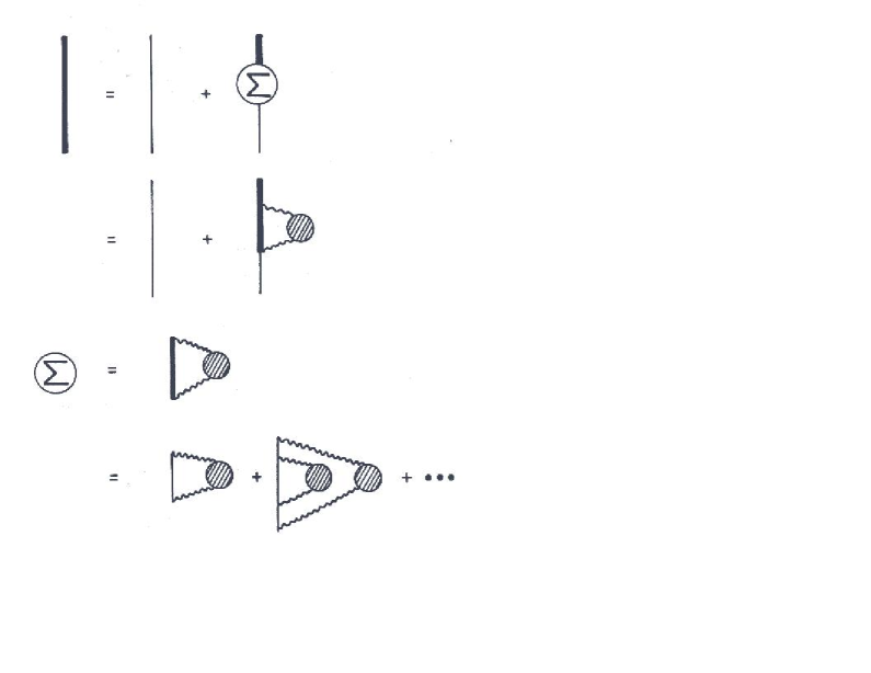
Figure 1: Equations for the ensemble-averaged quark propagator and the self-energy in the random-coupling model. a) The solid line is the full propagator and the light line is the propagator $[\hbox to0.0pt{\hbox to5.03125pt{\hfil/\hfil}\hss}p-m_{q}^{cur}]^{-1}$. b) A self-consistent model for the (irreducible) self-energy $\Sigma(p^{2})$. The cross-hatched circle denotes the condensate and the wavy lines are condensate gluons of zero momentum. c) Here we show the type of nested diagrams which are summed in this model for the self-energy $\Sigma(p^{2})$.

The translation of this analysis to a study of the quark propagator is immediate. We define a free propagator, $S^{(0)}(x,x^{\prime})$, and the ensemble average of the correlation function of the Heisenberg fields:

$$<S(x,x^{\prime})>=<\widetilde{vac}\mid T(\psi(x)\bar{\psi}(x^{\prime}))\mid\widetilde{vac}>.$$ (3.20)

The random element, $L_{1}$, is

$$L_{1}=g\mathbb{A}_{a}^{\mu}(x)\gamma_{\mu}\lambda^{a}/2.$$ (3.21)

We write

$$\Gamma_{\mu\nu}^{ab}(1,2) = <\widetilde{vac}\mid g^{2}\mathbb{A}_{\mu}^{a}(0)\mathbb{A}_{\gamma}^{b}(0)\mid\widetilde{vac}>$$ (3.22)

$$= -\frac{g_{\mu\nu}}{4}g^{2}\phi_{0}^{2}\frac{\delta_{ab}}{8}.$$ (3.23)

Here we have generalized the scalar correlation function, $\Gamma(1,2)$, to a form appropriate in the case the correlation functions involves random functions with color and Lorentz indices. In momentum space we have

$$S^{(0)}(p)=\frac{1}{\hbox to0.0pt{\hbox to5.03125pt{\hfil/\hfil}\hss}p},$$ (3.24)

and

$$<S(p)>\,=\frac{1}{\hbox to0.0pt{\hbox to5.03125pt{\hfil/\hfil}\hss}p-\Sigma(p)}.$$ (3.25)

We need not include an $i\epsilon$ in the denominators on the right-hand side of Eqs. (3.24) and (3.25) since we will consider solutions for $<S(p)>$ which have no singularities for real $p^{2}$. This feature of the analytic structure of the propagator is analogous to that found when studying classical wave propagation in a random medium [10], as noted earlier.

IV The Quark Self-Energy in The Kraichnan Random-Coupling Approximation

The approximation considered here is shown in Fig. 1. There the cross-hatched region denotes the condensate and the wavy lines are condensate gluons. When translated into momentum space, the assumption of large correlation length $(L\rightarrow\infty)$ means that the condensate gluons may be taken to carry zero momentum.

We write the quark self-energy as

$$\Sigma(p)=A(p^{2})\hbox to0.0pt{\hbox to5.03125pt{\hfil/\hfil}\hss}p+B(p^{2}).$$ (4.1)

In the random-coupling approximation we have [See Fig. 1],

$$A(p^{2})\hbox to0.0pt{\hbox to5.03125pt{\hfil/\hfil}\hss}p+B(p^{2})=-\kappa^{2}\gamma_{\mu}\frac{1}{\hbox to0.0pt{\hbox to5.03125pt{\hfil/\hfil}\hss}p-A(p^{2})\hbox to0.0pt{\hbox to5.03125pt{\hfil/\hfil}\hss}p-B(p^{2})-m_{q}^{cur}}\gamma^{\mu},$$ (4.2)

where $m_{q}^{cur}$ is a “current” quark mass and $\kappa^{2}\equiv g^{2}\phi_{0}^{2}/24$ contains a color factor of $4/3$.

Let us first consider the case $m_{q}^{cur}=0$. We see that Eq. (4.2) exhibits a bifurcation phenomenon. There is a solution with $B=0$; however, we will consider another solution with $B\neq 0$, which breaks chiral symmetry. That solution is

$$A(p^{2}) = -1\,,$$ (4.3)

$$B(p^{2}) = 2\sqrt{p^{2}+\kappa^{2}},\,\,\,\,\,\,\,\,\,\,\,\,\,\,\,\mbox{for}\,\,p^{2}\,>\,-\kappa^{2}.$$

and

$$A(p^{2}) = \frac{1}{2}\left[1-\sqrt{1-8\kappa^{2}/p^{2}}\right],$$ (4.4)

$$B(p^{2}) = 0,\,\,\,\,\,\,\,\,\,\,\,\,\mbox{for}\,\,p^{2}\,<\,-\kappa^{2}.$$

It is useful to define a dynamical mass

$$M(p^{2})=\frac{B(p^{2})+m_{q}^{cur}}{1-A(p^{2})},$$ (4.5)

which for $m_{q}^{cur}=0$ is

$$M(p^{2})=(p^{2}+\kappa^{2})^{1/2}\theta(p^{2}+\kappa^{2}).$$ (4.6)

It may be seen that Eqs. (4.3)-(4.4) represent the $m_{q}^{cur}=0$ limit of a continuous solution of Eq. (4.2) obtained with $m_{q}^{cur}\neq 0$. Equation (4.2) may be solved for $m_{q}^{cur}\neq 0$. One finds that $M(p^{2})$ satisfies a fourth-order polynomial equation. That equation has four solutions for each $p^{2}$. We choose a real continuous solution such that $M(p^{2})\rightarrow m_{q}^{cur}$ as $p^{2}\rightarrow-\infty$. The value of $M^{2}(p^{2})$, $B(p^{2})$ and $[1-A(p^{2})]$ for such solutions are shown in Figs. 2 to 14, for various values of $m_{q}^{cur}$. The values chosen are appropriate for up, down, strange, charm and bottom quarks. [We have also taken $\kappa^{2}$=(232 Mev)².]

We note that for the solutions chosen, for large spacelike $p^{2}$ we have $A(p^{2})\rightarrow 0,B(p^{2})\rightarrow 0$ and

$$<S(p)>\simeq\frac{1}{\hbox to0.0pt{\hbox to5.03125pt{\hfil/\hfil}\hss}p-m_{q}^{cur}}.$$ (4.7)

For timelike $p^{2}$ we have $M(p^{2})\rightarrow p^{2}+\kappa^{2}$ for large $p^{2}$. It may be seen that the equation $p^{2}=M^{2}(p^{2})$ has no solution and therefore there are no poles in the statistically averaged quark propagator for real $p^{2}$. This generalizes the corresponding result of the classical theory to the relativistic theory.

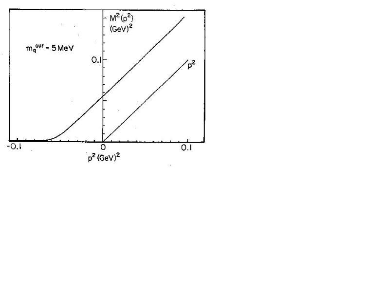
Figure 2: The square of the dynamical mass, $M^{2}(p^{2})$, for up and down quarks. Here we chose $m_{q}^{cur}$=5 MeV. [For $p^{2}>0$, $M^{2}(p^{2})=p^{2}+\kappa^{2}$.]

V Discussion

In this work we have shown that the ensemble average of the quark propagator exhibits damping. A similar result was obtained for the gluon propagator in an earlier work [12] where we used the first-order smoothing approximation [13] to generate an expression for the vacuum polarization operator. In Ref. [12] we studied the gluon propagator in momentum space and carried out a Fourier transformation to coordinate space. In that case one could see explicitly how the absence of on-mass-shell singularities in the propagator leads to damping of the wave both for spacelike and timelike propagation. In that analysis, carried in the Landau gauge, it was seen that the gluon obtained a dynamical mass $m_{G}^{2}=g^{2}\phi_{0}^{2}/4$. We also note that in a lattice simulation of $SU_{c}$(3) Yang-Mills theory in the Landau gauge [14] it was found the the gluon obtained a dynamical mass of $m_{G}=600\pm 90$ MeV. Since we had put $\kappa^{2}=g^{2}\phi_{0}^{2}/24$, we use this information to fix the value of $\kappa$ [$\kappa$=232 MeV].

In the work reported here we find that the solution which exhibits nonpropagation of quarks over large distances is also characterized as having $B\neq 0$. Nonzero values for $B$ denote chiral symmetry breaking. It is seen that only a single parameter, $g^{2}\phi_{0}^{2}$, governs both phenomena. This is a satisfactory result in the case of QCD, since only a single dynamically generated dimensionful parameter should characterize the theory.

Acknowledgment This work was supported in part by a grant from the Faculty Award Research Program of the City University of New York awarded to Xiangdong Li.

References

(1)L.S.Celenza and C. M. Shakin, Phys. Rev. D 34, 1591(1986).
(2)L.S.Celenza and C. M. Shakin, Effective Lagrangian Methods in QCD,
in Chiral Solitons, edited by Keh-Fei Liu, (World
Scientific, Singapore, 1987)
(3)Ph. Boucaud, A Le Yaouanc, J. P. Leroy, J. Micheli, O. Pne, and
J. Rodriguez-Quintero, Phys. Lett. B 493, 315(2000).
(4)K.-I. Kondo, Phys. Lett. B 514, 335(2002)
(5)A. A. Slavov, Gauge invariance of dimension two condensate in
Yang-Mills theory, hep-th/0407194.
(6)F. V. Gubarev, L. Stodolsky, and V. I. Zakharov, Phys. Rev.
Lett.86, 2220 (2001)
(7)F. V. Gubarev, V. I. Zakharov, Phys. Lett. B 501, 28(2001).
(8)E. R. Arriola, P. O. Bowman, and W. Broniowski, hep-ph/0408309.
(9)E. V. Shuryak, The QCD Vacuum, Hadrons and the
Superdense Matter (World Scientific, Singapore, 1988) and
references therein.
(10)U. Frisch, in Probabilistic Methods in
Applied Mathematics, edited by A. T. Bharucha-Reid
(Academic Press, New York, 1968), page 75.
(11)R. H. Kraichnan, J. Math. Phys. 2,124(1961).
(12)L. S. Celenza, C. M. Shakin, Hui-Wen Wang and
Xin-hua Yang, Intl. J. Mod. Phys. A 4, 3807(1989).
(13)R. C. Bourret, Nuovo Cim. 26, 1(1962).
(14)J. Mandula and M. Ogilvie, Phys. Lett. 185,
127(1987); R. Gupta, G. Guralnik, G. Kilcup, A. Patel, S. R.
Sharpe and T. Warnock, Phys. Rev. D 36, 2813(1987)