Quark recombination and elliptic flow

Abstract

Elliptic flow systematics for different hadron species have been explained by quark coalescence models. It has been argued that the elliptic asymmetry $v_{2}$ should scale with the number of quarks that comprise the hadron. We show how these arguments are sensitive to the relative role of asymmetries in the phase space density vs. asymmetries in the effective volume of emission. We also discuss the degree to which coalescence arguments differ from thermal models. Illustrative calculations based on solving the Boltzmann equation are presented along with the results of blast-wave models. Although the issue is complicated, ambiguities might be clarified by measurements of source-size parameters for nucleons at higher transverse momenta.

I Introduction

One of the surprising early measurements from RHIC shows that the proton/pion ratio reaches or even exceeds unity for transverse momenta $p_{t}$ above 2 GeV/c poverpidata . One explanation for this phenomena is that quarks originating from different nucleon-nucleon collisions recombine via coalescence mechanisms voloshin ; muellergroup ; kogroup . If this is indeed the explanation, it will make a case for having created a new state of matter where memory of the original color singlet hadrons is lost as the constituent partons become deconfined before going through a “mix-and-match” process, referred to as quark recombination.

Coalescence arguments have also been invoked to explain systematics of elliptic flow asymmetries voloshin ; muellergroup ; friesasymmetry ; kogroup ; molnar . These analyses are based on the parameter ollit ; volozh ,

$$v_{2}(p_{t})\equiv\frac{\int d\phi\left(dN/d\phi dp_{t}\right)\cos 2\phi}{\int d\phi\left(dN/d\phi dp_{t}\right)},$$ (1)

where the azimuthal angle $\phi$ is measured relative to the reaction plane. It is argued that if the underlying quarks have an asymmetry $v_{2}^{(q)}$, hadrons will have an asymmetry voloshin ; molnar ; friesasymmetry ,

$$v_{2}^{(n_{q})}(p_{t})=n_{q}v_{2}^{(q)}(p_{t}/n_{q}),$$ (2)

where $n_{q}$ is the number of quarks comprising the hadron. This might explain the fact that baryons seem to have $\sim 50\%$ higher asymmetries than mesons expv2scaling .

The main purpose of this paper is to investigate the validity of the scaling relation for $v_{2}$ of Eq. (2). Aside from the usual caveats concerning coalescence, Eq. (2) requires an assumption that the average phase space density has the same asymmetry as the invariant spectra. After demonstrating how this assumption plays a role we present sample calculations to illustrate the circumstances under which Eq. (2) is valid. For blast-wave models of the emitting state schn ; huovinen ; csorgo ; lisaretiere , we will show that the validity is sensitive to seemingly arcane choices of how to parameterize the model. Boltzmann equations are also solved for the partonic evolution where validity of Eq. (2) is found to be sensitive to the initial conditions.

The next section presents a discussion of quark recombination through coalescence with an emphasis on explaining the subtle differences between coalescence and thermal models. The subsequent sections present results from the blast-wave and Boltzmann calculations respectively. Results are summarized in Sec. V.

II Theory: Coalescence and Elliptic Flow

Coalescence arguments have been applied in numerous instances schwarz ; gyulassy ; dani ; nagle ; kahana ; mattiello ; schaffner to problems of fragment production in nuclear physics. It has been especially successful in describing the systematics of light nuclei production in high energy heavy-ion collisions where a high degree of thermalization is attained and temperatures far exceed typical nuclear binding energies. Coalescence shares many features of thermal models, and in fact provides the same results in the limit of high temperature relative to the binding energy mekjian . Although the focus of this paper is quark coalescence, the theory discussed in this section can be equally well applied to the coalescence of nucleons to form deuterons or light clusters. The main theoretical difference with quark coalescence is that one must be more cognizant of the effects of the non-zero binding energy and of relativistic motion. Whereas the deuteron binding energy is only 2.2 MeV and the momentum components of the nucleon-nucleon relative wave function has most of its strength in the range of tens of MeV/c, constituent quarks may form hadrons whose mass differs from the sum of the constituent quark masses by many hundreds of MeV. Momentum components of the quark’s relative motion also tend to be in the range of hundreds of MeV/c. Furthermore, one must add the qualifier that hadrons cannot necessarily be expressed in terms of constituent quarks, which ignores the gluons, sea quarks or vacuum fluctuations of meson fields.

In this section we further outline some of the subtle issues mentioned above, but rather than focusing on these issues, we will mainly consider a simplified case where $n_{q}$ constituent quarks each of mass $m_{q}$ combine to form a hadron of mass $n_{q}m_{q}$. This allows us to sidestep some of the more delicate points about coalescence and derive some simple relations for the behavior of elliptic flow as a function of the number of quarks.

II.1 Review of Coalescence Theory

The meaning of the term coalescence varies somewhat throughout the literature schwarz ; gyulassy ; dani ; nagle ; kahana ; mattiello ; schaffner . For the purposes of our discussion, we assume that it refers to the formation of a bound state of two pre-existing constituents via the sudden approximation, i.e., at the moment of coalescence the binding interaction is turned on suddenly and the probability that constituents $a$ and $b$ will form a composite object $C$ is

$$f_{C}({\bf P}_{C},{\bf R},t_{c})=\int d^{3}rd^{3}q\>W_{ab}^{(C)}({\bf q},{\bf r})\>f_{a}(m_{a}{\bf P}_{C}/(m_{a}+m_{b})+{\bf q},{\bf R}+{\bf r}/2,t_{c})f_{b}(m_{b}{\bf P}_{C}/(m_{a}+m_{b})-{\bf q},{\bf R}-{\bf r}/2,t_{c}).$$ (3)

Here, the phase space densities are denoted by $f_{i}$ and $W$ refers to the Wigner decomposition of the relative squared wave function. ${\bf P}_{C}$ is the momentum of the composite object, $t_{c}$ the coalescence time, and $\bf R$ and $\bf r$ are the center-of-mass and relative coordinates. Although this expression is non-relativistic, the problem can be considered in a frame where the velocity of the constituent particle $V$ is zero or small.

If the characteristic spread of the relative momenta and relative coordinates in $W({\bf q},{\bf r})$ are small compared to the scale of the initial momenta and spatial sizes, $W$ may be replaced with a delta function,

$$W_{ab}^{(C)}({\bf q},{\bf r})\approx\delta({\bf r})\delta({\bf q}).$$ (4)

The simplified coalescence formula is then,

$$f_{C}({\bf P}_{C},{\bf R},t_{c})\approx f_{a}(m_{a}{\bf P}_{C}/(m_{a}+m_{b}),{\bf R},t_{c})\>f_{b}(m_{b}{\bf P}_{C}/(m_{a}+m_{b}),{\bf R},t_{c}).$$ (5)

For a thermal source, we consider a Boltzmann form for the phase space density,

$$f_{i}(m_{i}{\bf V},{\bf R},t_{c})=\exp\left[-(E^{\prime}_{i}-\mu_{i}({\bf R},t_{c}))/T({\bf R},t_{c})\right],$$ (6)

where $E^{\prime}$ refers to the energy in the frame of the thermalizing medium. Inserting the thermal forms for $f_{a}$ and $f_{b}$ in Eq. (5) nearly reproduces the thermal form for $f_{C}$ with $\mu_{C}=\mu_{a}+\mu_{b}$. It differs by the factor $\exp(-B^{\prime}/T)$ where $B^{\prime}$ is the binding energy measured in the frame of the thermalized medium,

$$B^{\prime}=E^{\prime}_{a}+E^{\prime}_{b}-E^{\prime}_{C}.$$ (7)

For the coalescence of nucleons into deuterons, the binding energy of 2.2 MeV is much smaller than the temperature, making the coalescence and thermal forms nearly indistinguishable.

The source-function formalism, which is commonly used in two-particle correlations llope , can also be applied to this problem. In this formalism the last scatterings with third bodies are treated as randomizing interactions which can place the particles into bound states. The source functions are defined in terms of the quantum $T$ matrices which describe the scattering from third bodies into the final two-body state. The momentum distribution of a composite object created from two particles,

$$\frac{dN^{(C)}}{d^{3}p_{C}}=\sum_{f^{\prime}}\left|\int d^{4}x_{a}d^{4}x_{b}\>T_{f^{\prime}}(x_{a},x_{b})U(x_{a},x_{b};p_{C})\right|^{2},$$ (8)

where $U(x_{a},x_{b};p_{C})$ is the evolution matrix for particles evolving from space-time points $x_{a}$ and $x_{b}$ into the asymptotic state of a bound particle, $C$, with momentum $p_{C}$. The remainder of the system will evolve into the state $f^{\prime}$. By imposing the condition that the sources are independent, (apart from the final-state interaction), the $T$ matrices can be expressed as a product,

$$T_{f^{\prime}}(x_{a},x_{b})\rightarrow T_{f^{\prime}_{a}}(x_{a})T^{*}_{f^{\prime}_{b}}(x_{b}),~{}~{}~{}\sum_{f^{\prime}}\rightarrow\sum_{f^{\prime}_{a},f^{\prime}_{b}},$$ (9)

where $f^{\prime}_{a}$ and $f^{\prime}_{b}$ refer to the two independent sources of the particles $a$ and $b$. Inserting the factorized form into Eq. (8),

$$\frac{dN^{(C)}}{d^{3}p_{C}} = \sum_{f_{a},f_{b}}\left|\int d^{4}x_{a}d^{4}x_{b}\>T_{f_{a}}(x_{a})T_{f_{b}}(x_{b})U(x_{a},x_{b};p_{C})\right|^{2}$$ (10)

$$= \sum_{f_{a},f_{b}}\left|\int d^{4}x_{a}d^{4}x_{b}T_{f_{a}}(x_{a})T_{f_{b}}(x_{b})\exp\left[i(p_{a}+p_{b})\cdot(m_{a}x_{a}+m_{b}x_{b})/(m_{a}+m_{b})\right]u_{C}(x^{\prime}_{a}-x^{\prime}_{b})\right|^{2},$$

where the two scattering centers evolve into states $f^{\prime}_{a}$ and $f^{\prime}_{b}$. The center-of-mass behavior has been factored out of the evolution matrix, and $u$ is the evolution matrix in the frame where ${\bf P}_{C}=0$, with $X^{\prime}_{a}-X^{\prime}_{b}$ referring to the coordinates measured in that frame. (If the sources are not independent, there would have been correlations in the emission of $a$ and $b$ in the absence of final-state interactions.)

Invoking properties of Fourier transform,

$$\frac{dN^{(C)}}{d^{3}P_{C}} = \frac{1}{(2\pi)^{4}}\int d^{4}X_{a}d^{4}X_{b}d^{4}rd^{4}q\>S_{a}(m_{a}P_{C}/(m_{a}+m_{b})+q,X_{a})S_{b}(m_{b}P_{C}/(m_{a}+m_{b})-q,X_{b})e^{-iq\cdot r}$$

$$~{}~{}~{}~{}~{}~{}~{}~{}\times u^{*}(X^{\prime}_{a}-X^{\prime}_{b}+r^{\prime}/2)u(X^{\prime}_{a}-X^{\prime}_{b}-r^{\prime}/2);$$

$$S_{i}(p_{i},X) \equiv \sum_{f_{a}}\int d^{4}xT_{f_{i}}^{*}(X+x/2)T_{f_{i}}(X-x/2)e^{-ip_{i}\cdot X}.$$ (11)

When the source function $S_{i}(p,x)$ is evaluated on-shell, $p_{0}=E_{p}$, it can be identified with the probability of emitting a particle of type $i$ with momentum ${\bf p}$ from space-time point $x$.

A more tractable expression can be obtained by applying the smoothness approximation prattsmoothness ; wiedemannsmoothness ,

$$S_{a}(m_{a}P_{C}/(m_{a}+m_{b})+q,X_{a})S_{b}(m_{b}P_{C}/(m_{a}+m_{b})-q,X_{b})\approx S_{a}(m_{a}P_{C}/(m_{a}+m_{b}),X_{a})S_{b}(m_{b}P_{C}/(m_{a}+m_{b}),X_{b}).$$ (12)

This permits changing the integral over $q$ into a delta function which sets $r^{\prime}$ to zero. Equation (II.1) can then be written as

$$\frac{dN^{(C)}}{d^{3}P_{C}}=\int d^{4}X_{a}d^{4}X_{b}\>S_{a}(m_{a}P_{C}/(m_{a}+m_{b}),X_{a})S_{b}(m_{b}P_{C}/(m_{a}+m_{b}),X_{b})|u_{C}(X^{\prime}_{a}-X_{b}^{\prime})|^{2}.$$ (13)

This approximation is exact for thermal sources, since the Boltzmann factor is only a function of $P_{a}+P_{b}$, and is independent of the relative momentum.

Unfortunately, the evolution matrix $u_{C}(X^{\prime}_{a}-X^{\prime}_{b})$ involves a time difference. If the two times $t^{\prime}_{a}$ and $t^{\prime}_{b}$ are equal, $u$ can be replaced with the relative wave function which is often a well-understood object. A third approximation can then be made by introducing time independent evolution matrix $\phi$, i.e.,

$$|u_{C}(X^{\prime}_{a}-X^{\prime}_{b})|^{2}\approx(2\pi)^{3}|\phi_{C}({\bf X}^{\prime}_{a}-{\bf X}^{\prime}_{b})|^{2}.$$ (14)

Without this last approximation it would have been essential to understand the details of the evolution of the particles for times between the emissions of the first and second particle. Since the particles are, by definition, not moving rapidly in this frame, the wave function at this time should not change substantially and this should be a reasonable approximation. Putting the three approximations together, i.e., source factorization, smoothness, and ignoring of the offsets of emission times, we obtain an expression similar to that used in correlation studies

$$\frac{dN^{(C)}}{d^{3}P_{C}}=(2\pi)^{3}\int d^{4}X_{a}d^{4}X_{b}\>S_{a}(m_{a}P_{C}/(m_{a}+m_{b}),X_{a})S_{b}(m_{b}P_{C}/(m_{a}+m_{b}),X_{b})|\phi_{C}({\bf X}^{\prime}_{a}-{\bf X}^{\prime}_{b})|^{2}.$$ (15)

After approximating the squared relative wave function as a $\delta$ function, and noting that the phase space density can be related to the source function by the relation,

$$f_{a}(m_{a}{\bf P}_{C}/(m_{a}+m_{b}),{\bf x},t_{c})=(2\pi)^{3}\int d^{4}X_{a}\>S_{a}(E_{a},m_{a}{\bf P}_{C}/(m_{a}+m_{b}),X_{a})\delta({\bf x}-{\bf X}-{\bf v}(t_{c}-X_{0})),$$ (16)

the coalescence formula of Eq. (5) would be reproduced, except that the source function in Eq. (15) is evaluated off-shell.

$$m_{a}E_{C}/(m_{a}+m_{b})\neq E_{a}(m_{a}{\bf P}_{C}/(m_{a}+m_{b})).$$ (17)

Within the smoothness approximation, there is no difference in replacing the energy arguments of the source functions in Eq. (15) with on-shell values.

For a thermal source, the product of the source functions becomes a Boltzmann factor, $\exp(-E_{C}/T)$, and hence Eq. (15) is equivalent to a thermal expression. Thus, the coalescence expression, Eq. (3), the thermal expression, Eq. (6), and the source function expression, Eq. (15), become equivalent for thermal distributions when the binding energy is zero. The lack of dependence on the binding energy in coalescence formulas is due to the sudden approximation, which presumes that the binding potential is turned on suddenly, i.e., energy is not conserved. From a quantum perspective, the source function in Eq. (16) is found by factoring quantum matrix elements with the density of states. If the matrix elements are assumed to be featureless, and if the density of states of the sources behaves as $\exp(E/T)$, a thermal form is then obtained. When forming hadrons, it is hard to argue that the interactions with third bodies do not provide some additional leverage for creating final states with larger binding energies, i.e., the phase space density of protons should be greater than that of deltas. As can be garnered from the list of approximations above, neither the coalescence expression nor the thermal expression can be justified to better than the 10% level. Moreover, once a decision has been made regarding the choice of one of the formalisms, additional choices must be made for parameters such as the temperature and rest frame of the thermal source. For the coalescence formula it is necessary to make a choice of a rest frame for the coalescence. In this Lorentz frame the interaction between $a$ and $b$ turns on instantaneously. Momentum is conserved, but energy is not conserved. In all other frames, neither energy nor momentum are conserved. Again, it should be stressed that these subtle sensitivities to parameters and choice of reference frames disappear when the binding energy is small.

To illustrate the sensitivity of coalescence pictures to binding energy, let us consider the extreme case of two constituent quarks of mass 350 MeV coalescing to form a pion. If the quarks are to coalesce in the two-particle rest frame, the energy will change by 60% from the coalescence in that frame. If the coalescence is observed in the lab frame, the pair will loose 60% of its momentum in the coalescence process. Whereas, if the coalescence frame is the laboratory frame, the laboratory momentum of the two quarks will be conserved in this process. Although, pions are an extreme example, most coalescence pictures involve mass changes at the 20% level, which provides a feel for the confidence with which one can apply coalescence prescriptions.

Whether recombination is thermal or sudden by nature, the two expressions share an important property. Both formulas presume that the $a$ and $b$ components exist independently of one another. This will not be true if the partons, for example, originate from the same jet. It is the validity of the factorization that is related to whether or not hadronization can be described as the recombination of partons without regard to whether the two owe their existence to the same initial nucleon-nucleon collision. For many of the calculations presented in the following sections, the issue of thermal vs. sudden will be side-stepped by focusing on the coalescence of two quarks with constituent masses $m_{q}$ which combine to make a meson of mass $2m_{q}$.

II.2 Coalescence and Elliptic Flow

In this subsection, and in the examples presented in the next section, we consider the coalescence of $n_{q}$ quarks into a hadron of mass $M_{C}=n_{q}m_{q}$, where $m_{q}$ is the constituent quark mass. Thus, we ignore many of the subtle issues concerning the binding energy, and the relative merits of one formalism with another. The expression analogous to Eq. (5) for the coalescence of $n_{q}$ quarks is

$$f_{C}({\bf P},{\bf R},t)\approx\left[f_{q}(m_{q}{\bf P}/M_{C},{\bf R},t)\right]^{n_{q}}.$$ (18)

The hadron spectra is found by integrating the phase space density over coordinate space,

$$\frac{dN_{C}}{d^{3}P} = \frac{(2S_{C}+1)}{(2\pi)^{3}}\int d^{3}rf_{C}({\bf P},{\bf r},t)$$ (19)

$$= \frac{(2S_{C}+1)}{(2\pi)^{3}}\int d^{3}r\left[f_{q}({\bf P}/n_{q},{\bf R},t)\right]^{n_{q}},$$

where $S_{C}$ is the spin of the composite particle $C$.

The principal goal of this paper is to investigate the behavior of the angular asymmetry which is quantified by the parameter $v_{2}$ defined in Eq. (1). If the composite particle is made up of $n_{q}$ quarks, each with the same phase space density $f_{q}$, we have from Eqs. (1) and (19)

$$v_{2}^{(n_{q})}(p_{t})=\frac{\int d\phi d^{3}r\left[f_{q}(p_{t}/n_{q},\phi,{\bf r},t_{c})\right]^{n_{q}}\cos 2\phi}{\int d\phi d^{3}r\left[f_{q}(p_{t}/n_{q},\phi,{\bf r},t_{c})\right]^{n_{q}}},$$ (20)

where $\phi$ refers to the azimuthal angle of the momentum.

The phase space density can be written as a product of the spectra and an effective density, $\rho_{q}({\bf r},y_{t},\phi)$, defined by the relation,

$$\rho_{q}({\bf r},y_{t},\phi)\equiv\frac{f_{q}(y_{t},\phi,{\bf r})}{(2\pi)^{3}(dN^{(q)}/d^{3}p)}.$$ (21)

Here, $\rho_{q}$ is non-zero over the region where particles are emitted. If the phase space density is constant within a fixed volume, $\Omega$, then $\rho_{q}=1/\Omega$. If $\rho_{q}$ is independent of $\phi$, $v_{2}^{(C)}$ can be written in terms of the quark spectra,

$$v_{2}^{(n_{q})}(y_{t})=\frac{\int d\phi\left[dN^{(q)}/d^{3}p\right]^{n_{q}}\cos 2\phi}{\int d\phi\left[dN^{(q)}/d^{3}p\right]^{n_{q}}},$$ (22)

where $dN^{(q)}/d^{3}p$ is evaluated for quarks at a fixed transverse rapidity, $y_{t}$. If the quark spectra has an elliptic asymmetry as $dN^{(q)}/d^{3}p\propto(1+\epsilon\cos 2\phi)$, then $v_{2}^{(q)}=\epsilon/2$ and $v_{2}^{(n_{q})}$ can be expressed in terms of $v_{2}^{(q)}$,

$$v_{2}^{(n_{q})} = \frac{\int d\phi\>\left[1+2v_{2}^{(q)}\cos 2\phi\right]^{n_{q}}\cos 2\phi}{\int d\phi\left[1+2v_{2}^{(q)}\cos 2\phi\right]^{n_{q}}}$$ (23)

$$= \frac{1}{2}\frac{\sum_{n=1,3,\cdots}^{n_{q}}(n+1)\left(v_{2}^{(q)}\right)^{n}\frac{n_{q}!}{(n_{q}-n)!\left([(n+1)/2]!\right)^{2}}}{\sum_{n=0,2,\cdots}^{n_{q}}\left(v_{2}^{(q)}\right)^{n}\frac{n_{q}!}{(n_{q}-n)!\left[(n/2)!\right]^{2}}}.$$

For $n_{q}=2,3$, the expression becomes molnar

$$v_{2}^{(2)} = 2v_{2}^{(q)}\frac{1}{1+2(v_{2}^{(q)})^{2}}$$

$$v_{2}^{(3)} = 3v_{2}^{(q)}\frac{1+(v_{2}^{(q)})^{2}}{1+6(v_{2}^{(q)})^{2}}.$$ (24)

For small $v_{2}^{(q)}$ one obtains the simple scaling relation, Eq. (2).

It is this simple scaling relation that has been cited as evidence for quark recombination voloshin ; molnar ; friesasymmetry . However, the validity of this relation hinges on the assumption that the effective density is independent of $\phi$. The nature of this assumption can be understood by considering two examples illustrated in Fig. 1. In the left side the effective volumes for emission upwards and to the right are identical, and the higher number of particles emitted to the right is due to the higher average phase space density of those particles. Thus, for this example, the elliptic asymmetry for dimers will be double the elliptic asymmetry for monomers and will satisfy the scaling relation, Eq. (2). For the emission illustrated in the right panel of Fig. 1, the average phase space density for emission in the two directions are identical, and the higher number of particles emitted to the right is due to a larger effective volume. In this case, the asymmetry for monomers and dimers is the same.

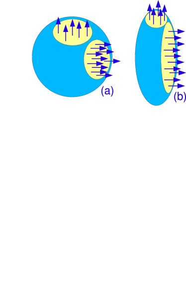
Figure 1: Two sources are illustrated above. The particles of a given velocity are represented by arrows. In (a) the effective volumes of the right-moving and upward-moving particles are the same but the right-moving particles have a higher phase space density. In (b) the phase space densities are the same but the effective volumes differ. In both cases there are twice as many particles moving to the right as upward so $v_{2}$ is identical. But in (a) the $v_{2}$ for a bound state of $n_{q}$ particles will increase by a factor of $n_{q}$ while in (b) the composite particle will have the same $v_{2}$ as the constituents.

To illustrate the same effect shown in Fig. 1 algebraically, let us consider a phase space density characterized by a Gaussian profile,

$$f_{q}(p_{t},\phi,{\bf r})=2^{3/2}\bar{f}(p_{t},\phi)\exp\left[-r^{2}/(2R^{2}(p_{t},\phi))\right],$$ (25)

where $\bar{f}$ is the phase space density averaged over the coordinate space. The probability for emitting a coalesced $n_{q}$-quark object is then

$$\frac{dN_{C}}{d^{3}p}=\frac{(2S_{C}+1)2^{3n_{q}/2}}{(2\pi n_{q})^{3/2}}R^{3}(p_{t},\phi)\left[\bar{f}(p_{t},\phi)\right]^{n_{q}}.$$ (26)

If $v_{2}^{(\bar{f})}$ and $v_{2}^{(\Omega)}$ refer to the elliptic asymmetries of the average phase space density and effective volumes of the single quarks,

$$v_{2}^{(\bar{f})}(p_{t}) \equiv \frac{\int d\phi\>\bar{f}(p_{t},\phi)\cos 2\phi}{\int d\phi\>\bar{f}(p_{t},\phi)},$$

$$v_{2}^{(\Omega)}(p_{t}) \equiv \frac{\int d\phi\>R^{3}(p_{t},\phi)\cos 2\phi}{\int d\phi\>R^{3}(p_{t},\phi)},$$ (27)

the asymmetry for the $n_{q}$-quark object can be written as

$$v_{2}^{(n_{q})}=v_{2}^{(\Omega)}+n_{q}v_{2}^{(\bar{f})}.$$ (28)

Equation (28) is again based on the assumption that the asymmetries are not large, but includes the chance that the asymmetries can originate from either asymmetries of the effective volume or asymmetries of the average phase space density.

If the effective volumes are independent of $\phi$, $v_{2}^{(\Omega)}$ is zero. The Eqs. (23) and (28) are then identical and the asymmetry scales linearly with $n_{q}$. Such a case is illustrated in the left panel of Fig. 1. On the other hand, if the average phase space density is independent of $\phi$, $v_{2}^{(\bar{f})}$ is zero and the asymmetry is then independent of $n_{q}$. This will be the case for emissions of the type illustrated in the right panel of Fig. 1. Several examples are explored in the next section, with the purpose of understanding what drives the asymmetry, the effective volume or the average phase space density.

The effective volumes, $R^{3}$ in the Gaussian case, can be determined experimentally through correlation measurements starcor ; phenixcor ; lisa or with coalescence measurements llope ; stardbar ; palpratt . This volume can be defined in terms of the phase space density,

$$\Omega(y_{t},\phi)\equiv\frac{\left[\int d^{3}rf_{q}(y_{t},{\bf r})\right]^{2}}{\int d^{3}r[f_{q}(y_{t},{\bf r})]^{2}}.$$ (29)

For a Gaussian source of dimensions $R_{x}$, $R_{y}$ and $R_{z}$, $\Omega=2^{3/2}R_{x}R_{y}R_{z}$. In considering the coalescence of nucleons, rather than that of quarks, the volume may be determined with two-nucleon correlation measurements. The effective volume may be also estimated from coalescence ratios. The coalescence volume can be defined by the ratio of spectra of two particles $a$ and $b$ that combine to form a coalesced object $C$ as can be seen in Eq. (29),

$$\Omega=\frac{(2S_{C}+1)}{(2S_{a}+1)(2S_{b}+1)}\frac{(dN_{a}/d^{3}p)(dN_{b}/d^{3}p)}{dN_{C}/d^{3}P}.$$ (30)

For small asymmetries, this yields $v_{2}^{(\Omega)}=v_{2}^{(a)}+v_{2}^{(b)}-v_{2}^{(C)}$, which is basically a tautological restatement of Eq. (28). Other methods for measuring the source size as a function of the azimuthal angle, will provide independent means for determining whether the $v_{2}^{(\Omega)}$ is independent of $\phi$. Examples of such methods are identical pion correlations or proton-lambda correlations.

III Blast Wave Models

Blast wave descriptions schn ; huovinen ; csorgo ; lisaretiere , provide a simple means by which one can test thermal concepts along with those for collective flow. Typically, a blast-wave model requires four parameters: a temperature $T$, a breakup time $\tau$, a transverse radius $R$ and a maximum transverse collective rapidity, $\rho_{0}$. When considering elliptic asymmetries, one may also use two parameters for the transverse radii, $R_{x}$ and $R_{y}$, and two parameters to describe the transverse collective motion. There are many variants of blast-wave models that differ from the form by which the space-time distributions are parameterized. Of the three parameterizations considered here, each assumes that the distribution of thermal sources is invariant to boosts along the beam directions. Although the choice of the form seems somewhat arbitrary when analyzing spectra, we find that the different forms result in rather different behavior in the elliptic flow.

III.1 Shell parameterization for the blast-wave

Asymmetries can be added to a thermal blast-wave in four independent ways via the temperature, the collective velocity, the chemical potential, or the volume. To compare the effects of these four types of asymmetries, we consider a simple azimuthally symmetric shell

$$\frac{dN}{d\phi_{p}dp_{t}}\sim\int d\phi_{u}d\eta\>\cosh\eta\>\rho_{s}(\phi_{u})\exp\!\left[\frac{-\cosh\eta\>m_{t}\sqrt{1+u_{\perp}^{2}(\phi(s))}+u_{\perp}(\phi_{u})p_{t}\cos(\phi_{p}-\phi_{u})}{T(\phi_{u})+n\mu(\phi_{u})/T(\phi_{u})}\right].$$ (31)

Here $u_{\perp}$ is the transverse collective velocity, $\rho(\phi_{u})$ is the angular density for sources having a collective flow in the radial direction $\phi_{u}$ and $\eta$ is the longitudinal rapidity of the source. The four asymmetries can be parameterized in the following way,

$$\rho(\phi_{u}) = (1+\epsilon_{V}\cos 2\phi_{u})\rho,$$

$$\exp\!\left[\mu(\phi_{u})/T(\phi_{u})\right] = (1+\epsilon_{\mu}\cos 2\phi_{u})\exp(n_{q}\mu/T),$$

$$T(\phi_{u}) = (1+\epsilon_{T}\cos 2\phi_{u})T,$$

$$u_{\perp}(\phi_{u}) = (1+\epsilon_{u}\cos 2\phi_{u})u_{\perp}.$$ (32)

Inserting these equations into (31), the expressions are then expanded to lowest power in $\epsilon$ which allows the integrals to be performed analytically. The resulting expressions for each of the four expansion are:

$$v_{2,V} = \epsilon_{V}\frac{J_{V}}{J_{0}},$$

$$v_{2,\mu} = n_{q}\epsilon_{\mu}\frac{J_{V}}{J_{0}},$$

$$v_{2,T} = \epsilon_{T}\left(\frac{m_{t}\sqrt{1+u_{\perp}^{2}}}{T}J_{E}-\frac{u_{\perp}p_{t}}{T}J_{p}\right)\frac{1}{J_{0}},$$

$$v_{2,u} = \epsilon_{u}\left(-\frac{u_{\perp}^{2}m_{t}}{T\sqrt{1+u_{\perp}^{2}}}J_{E}+\frac{u_{\perp}p_{t}}{T}J_{p}\right)\frac{1}{J_{0}},$$ (33)

where $J_{0}$, $J_{E}$ and $J_{p}$ are simple combinations of Bessel functions,

$$J_{0} = 2K_{1}(z_{E})I_{0}(z_{p}),$$

$$J_{V} = K_{1}(z_{E})I_{2}(z_{p}),$$

$$J_{p} = \frac{1}{2}K_{1}(z_{E})\left[I_{1}(z_{p})+I_{3}(z_{p})\right],$$

$$J_{E} = \left[K_{0}(z_{E})+K_{1}(z_{E})/z_{E}\right]I_{2}(z_{p}),$$ (34)

with $z_{E}=(m_{t}/T)\sqrt{1+u_{\perp}^{2}}$ and $z_{p}=u_{\perp}p_{t}/T$.

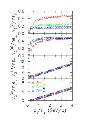
Figure 2: Scaled values for elliptic flow as a function of scaled transverse momentum for constituent quarks each of mass $m_{q}=350$ MeV coalescing to form composite objects of $n_{q}=1,2,3$ quarks with mass $M_{C}=n_{q}m_{q}$. Asymmetries are introduced into the cylindrical-shell parameterization of the blast-wave by adding elliptic distortions to the thickness of the envelope (upper panel), the density as driven by a chemical potential (second panel), the temperature (third panel) and the collective velocity (lower panel). Scaling is significantly violated for the upper two panels.

Figure 2 displays the resulting values of $v_{2}$ for each of the four asymmetries as a function of the scaled transverse momentum. For these calculations, the masses of the coalesced hadrons are assumed to be $n_{q}\times$ 350 MeV. By plotting $v_{2}/n_{q}$ vs. the $p_{t}/n_{q}$, satisfaction of quark-number scaling of Eq. (2) will provide indistinguishable lines for different values of $n_{q}$. The upper panel shows asymmetries from adding an elliptic distortion to $\rho(\phi_{u})$. This type of asymmetry will result from distorting the shape of the shell while keeping the magnitude of the collective velocity fixed, or by altering the thickness of the shell. Effectively, these distortions represent an elliptic asymmetry to the effective volumes of the source as described in Fig. 1. Scaling is then strongly violated since $v_{2}$ is approximately independent of $n_{q}$. In the second panel, results are shown for adding an elliptic asymmetry to the chemical potential. This is same as in the upper panel, except that it scales with an extra power of $n_{q}$ since the density enters as $\exp(\mu/T)$. Quark-number scaling then appears to be well satisfied except at low $p_{t}$.

The lower two panels of Fig. 2 show the result of elliptic distortions to the temperature $T$ and to the magnitude of the collective velocity $\bar{u}$. In both cases, quark-number scaling appears to be very well satisfied. But, in these cases, satisfaction of quark-number scaling is driven by the fact that $v_{2}$ rises linearly with $p_{t}$. If mass effects are neglected, $v_{2}$ can only depend on $p_{t}$ unless the chemical potential is varied, which will introduce an $n_{q}$ dependence. If $v_{2}$ rises linearly, scaling both the $x$ and $y$ axes by $1/n_{q}$ will yield a line with the same slope, and quark-number scaling should automatically be satisfied. In fact, universal curves will result if scaled by any number, but not just the quark number. It should be pointed out that the linear behavior with $p_{t}$ does not hold at low $p_{t}$, where $v_{2}$ must be quadratic. The region over which it appears quadratic depends on the collective velocity $\bar{u}$. For smaller $\bar{u}$ the quadratic region becomes noticeably larger.

Even though the asymmetries in temperature and collective velocity produce excellent linear results for $v_{2}$ vs. $p_{t}$, the superposition of several shells with different values of $\bar{u}$ and $T$ can lead to non-linear behavior for $v_{2}$ vs. $p_{t}$. This is because the slope can depend on the parameters, and by changing $p_{t}$, the relative contribution of one shell may increase with respect to another. When $v_{2}$ vs. $p_{t}$ is not linear, quark-number scaling is more significant.

III.2 Blast-Wave Parameterization of Retiere and Lisa

The next parameterization we present was used to analyze elliptic flow and correlations in lisaretiere . This model describes a uniform transverse density profile that is cut off by an elliptic surface. The normalized elliptical radius $\tilde{r}$ corresponding to a surface of constant $\tilde{r}$ is defined as

$$\tilde{r}=\sqrt{\frac{x^{2}}{R_{x}^{2}}+\frac{y^{2}}{R_{y}^{2}}}.$$ (35)

Emission is confined to the region where $\tilde{r}<1$. The transverse rapidity is defined to rise linearly from the origin,

$$y_{t}=\tilde{r}(\rho_{0}+\rho_{a}\cos 2\phi),$$ (36)

where the two parameters, $\rho_{0}$ and $\rho_{a}$ parameterize the collective flow with $\rho_{a}$ driving the asymmetry. The transverse velocity is then $u_{\perp}=\sinh(y_{t})$. The direction of the collective flow is chosen to be perpendicular to the surfaces of constant $\tilde{r}$.

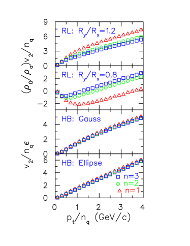
Figure 3: Scaled values for elliptic flow as a function of scaled transverse momentum for constituent quarks each of mass $m_{q}=350$ MeV coalescing to form composite objects of $n_{q}=1,2,3$ quarks with mass $M_{C}=n_{q}m_{q}$. A constant temperature of $T=100$ MeV is considered for all the calculations. The results are in the blast-wave model of Retiere and Lisa lisaretiere (upper two panels), and to a more hydrodynamically consistent parameterization (lower two panels). Quark-number scaling is better realized by the hydrodynamic parameterization. For the Retiere-Lisa parameterization, scaling is strongly violated when the ellipse becomes elongated in the in-plane direction.

The upper two panels of Fig. 3 show $v_{2}$ from this model with the parameters, $T=100$ MeV, $\rho_{0}=0.9$ and $\rho_{a}=0.1$. The calculations are for constituent quarks of mass $m_{q}=350$ MeV and with hadrons of mass $n_{q}m_{q}$. The results are independent of the proper time $\tau$ and are not independently sensitive to $R_{x}$ and $R_{y}$, but instead depend only on the ratio, $R_{y}/R_{x}$. If the matter falls apart quickly after the initial overlap of the colliding nuclei, then $R_{y}/R_{x}>1$. The upper panel of Fig. 3 with $R_{y}/R_{x}=1.2$ displays results for such a scenario. Here $v_{2}$ of the composite hadrons is calculated using the phase space density as described in Eq. (19), and then $v_{2}$ is divided by the number of constituent quarks. The scaling criteria of Eq. (2) is seen to be satisfied rather well in this case as all the curves lie close to one another.

At later times, the unequal transverse expansion will overcome the initial out-of-plane extended profile and reach an in-plane-extended geometry. The second panel of Fig. 3 displays the results for $R_{y}/R_{x}=0.8$. In this case, quark-number scaling is strongly violated. Moreover, $v_{2}$ becomes negative in some instances as was noted in lisaretiere . This peculiar behavior is due to the constraint that the collective flow is perpendicular to the constant $\tilde{r}$ surfaces. Thus, non-zero $v_{2}$ values even occur in the case where $\rho_{a}=0$.

The constraint that the collective flow is perpendicular to the surfaces of constant $\tilde{r}$ is not justified from the perspective of hydrodynamics. It is expected that the accelerations, which are driven by the density gradients, are perpendicular to the surface of the ellipse, rather than the velocities. For early times, before the shape has a chance to react to the acceleration, the transverse acceleration and velocities should be parallel to one another. But at later times, when $R_{y}/R_{x}$ approaches or exceeds unity, the constraint enforces a rather awkward velocity profile. This will be more apparent below where we consider the third parameterization.

III.3 Hydrodynamically Inspired Blast Wave

The second blast-wave model we will consider has the benefit of representing a solution to non-relativistic hydrodynamics csorgo . This parameterization represents a solution to hydrodynamic equations in the limit that $P=nT$, and particle number is conserved. Hydrodynamic can realize this form even if the thermal motion is relativistic. The form also works for the simple ultra-relativistic equation of state, $P\propto\epsilon$. However, this parameterization does not represent an exact solution in the limit of high collective velocities.

In this parameterization, the transverse profiles are Gaussian and the flow velocities rise linearly from the origin.

$$f \propto \frac{N}{(2\pi R_{x}R_{y})}\exp\!\left(-n_{q}\frac{x^{2}}{R_{x}^{2}}-n_{q}\frac{y^{2}}{R_{y}^{2}}\right)\exp(-E^{\prime}/T),$$

$$u_{x} = \alpha_{x}x,~{}u_{y}=\alpha_{y}y,$$ (37)

where $u_{x}$ and $u_{y}$ are the transverse relativistic velocities. As in the previous model, it is assumed that the matter disintegrates at a fixed temperature $T$. The factor $n_{q}$ in the exponential suggests that the space-time structure of the Gaussian is driven by a position-dependent chemical potential connected to the conserved quark number. In this parameterization the elliptic flow does not depend on the radii and collective flow parameters separately, but instead only on the combinations $\alpha_{x}R_{x}$ and $\alpha_{y}R_{y}$. Since the collective velocities scale simply with the space-time coordinates, it is straight-forward to express the spectra over integrals of the collective velocities,

$$\frac{dN}{d^{3}p}\sim\int d\eta\cosh\eta\>u_{\perp}du_{\perp}d\phi_{u}\exp\left[-\frac{m_{t}}{T}\sqrt{1+u_{\perp}^{2}}+\frac{u_{\perp}}{T}\cos(\phi_{u}-\phi_{p})-\frac{n_{q}u_{x}^{2}}{2\alpha_{x}R_{x}^{2}}-\frac{n_{q}u_{y}^{2}}{2\alpha_{y}R_{y}^{2}}\right],$$ (38)

where $\phi_{p}$ refers to the direction of the momentum and $\phi_{u}$ is the azimuthal direction of the transverse collective velocity $u_{\perp}$.

The integral can be performed analytically if the asymmetry is small. Defining the parameters $\bar{u}$ and $\epsilon$,

$$\bar{u} = \frac{1}{2}(\alpha_{x}R_{x}+\alpha_{y}R_{y}),$$

$$\alpha_{x}R_{x} = \bar{u}(1+\epsilon),~{}\alpha_{y}R_{y}=\bar{u}(1-\epsilon),$$ (39)

leads to an expression for which the angular integrals can be performed analytically after expanding to lowest power in $\epsilon$.

$$\frac{dN}{d^{3}p}\sim\int d\eta\cosh\eta\>u_{\perp}du_{\perp}d\phi_{u}\left(1+n_{q}\epsilon\frac{u_{\perp}^{2}}{\bar{u}^{2}}\cos(2\phi_{u})\right)\exp\!\left[-\frac{m_{t}}{T}\sqrt{1+u_{\perp}^{2}}+\frac{u_{\perp}}{T}\cos(\phi_{u}-\phi_{p})-\frac{u_{\perp}^{2}}{2\bar{u}^{2}}\right].$$ (40)

The calculation of $v_{2}$ involves an additional convolution with $\cos 2\phi_{p}$, and gives

$$v_{2} = n_{q}\epsilon\int u_{\perp}du_{\perp}(u_{\perp}^{2}/\bar{u}^{2})e^{-n_{q}u_{\perp}^{2}/2\bar{u}^{2}}K_{1}(z_{E})I_{2}(z_{p})/{\cal N},$$

$${\cal N} = 2\int u_{\perp}du_{\perp}e^{-n_{q}u_{\perp}^{2}/2\bar{u}^{2}}K_{1}(z_{E})I_{0}(z_{p}),$$

$$z_{E} = (m_{t}/T)\sqrt{1+u_{\perp}^{2}},~{}~{}z_{p}=u_{\perp}p_{t}/T.$$ (41)

Results for this prescription are displayed in the third panel of Fig. 3 for the case of a 350 MeV constituent quark mass. The temperature $T$ is considered the same as in the previous example and $\bar{u}$ is chosen to be 0.5. There is no peculiar negative elliptic flow from this parameterization, and constituent scaling appears to be maintained to a remarkably high level. Unlike the previous parameterization, we find no sensitivity to the ratio $R_{y}/R_{x}$.

It can be shown that for small flow velocities and non-relativistic temperatures, quark-number scaling becomes exact. However, this limit is far from realized, and the apparent scaling is only approximate.

To test the sensitivity of the scaling to the Gaussian shape of the profile, we repeated the calculation with an elliptic profile. For this calculation, the collective transverse rapidities are again chosen to rise linearly with the position, but the density is chosen to be uniform within an elliptic region. Also, as in the case of the Gaussian source, $v_{2}$ is independent of the spatial parameters. The results for the ellipse, shown in the lower panel of Fig. 3 are nearly identical to the Gaussian case. It thus appears that the crucial factor for scaling is that the collective velocity rises linearly with the position.

The fact that both the elliptic and Gaussian profiles are fairly successful at reproducing quark-number scaling may be surprising given that the Gaussian profile for the collective velocities has an explicit dependence on $n_{q}$, while the elliptic profile does not. Since the Gaussian profile behaves as $\exp(-n_{q}u^{2}/2\bar{u}^{2})$, the average collective flow decreases as $1/\sqrt{n_{q}}$. Lower collective flows result in lower values for $v_{2}$. However, since the distortions scale linearly with the density, $\sim(1+n_{q}\epsilon\cos 2\phi_{u})$, the two effects somewhat cancel one another to some extent, and one obtains values of $v_{2}$ which depend mainly on $p_{t}$. Since this dependence is roughly linear, scaling both the $x$ and $y$ axes by $n_{q}$, or any other constant, still results in a semi-universal curve.

Hydrodynamics provides for many more possibilities than the Gaussian density profile with linear velocity profiles as described above. A strong first-order phase transition will result in shock waves GulMat ; Rischke , which can strongly violate the assumption of linear velocity profiles. Additionally, the temperatures might not be independent of the position. Nonetheless, most full hydrodynamic solutions do tend to approach semi-linear forms by the time breakup is approached huovinen .

III.4 Sensitivity to Mass

In addition to the assumption that the effective volume referred to in Eq. (28) was independent of $\phi$, the scaling of $v_{2}$ with quark number requires that for a particle $C$ composed of particles $a$ and $b$,

$$f_{C}(M_{C}{\bf u},x)=f_{a}(m_{a}{\bf u},x)f_{b}(m_{b}{\bf u},x),$$ (42)

where ${\bf u}=\gamma{\bf v}$ is the relativistic velocity. For a thermal source where

$$f_{i}({\bf p},x)=\exp[-E^{\prime}_{i}/T(x)+(\mu_{i}(x)/T(x)],$$ (43)

Eq. (42) is satisfied with a thermal distribution if the three criteria are satisfied:

1. The temperatures describing $a$, $b$ and $C$ are the same.

2. The energies are conserved, $E_{C}(M_{C})\approx E_{a}(m_{a}P_{C}/(m_{a}+m_{b}))+E_{b}(m_{b}P_{C}/(m_{a}+m_{b}))$.

3. The chemical potential for $C$ is the sum of the constituent chemical potentials, $\mu_{C}(x)/T(x)=\mu_{a}(x)/T(x)+\mu_{b}(x)/T(x)$.

The first criteria requires only the assumption that the different species are kinetically thermalized.

Since the energies are a mass multiplied by the gamma factor describing the motion of the particles in the frame of the source at $x$, the second criteria can be re-stated as a requirement that the masses sum, $M_{C}=m_{a}+m_{b}$. This is equivalent to a requirement that there is no binding energy involved. However, even if binding energy is involved, another simple scaling can be derived, as discussed by Molnár molnar_mscaling . If the chemical potential is ignored, Eq. (43) may be written as

$$f_{\mu=0}(m_{a}{\bf u},x)=[f_{\mu=0}(m_{0}{\bf u},x)]^{m_{i}/m_{0}},$$ (44)

which then implies that if one can ignore the contribution to $v_{2}$ from the volume like term,

$$v_{2}^{(C)}=\frac{M_{C}}{m_{a}}v_{2}^{(a)}=\frac{M_{C}}{m_{b}}v_{2}^{(b)}.$$ (45)

For the case where the quark masses are the same, this results in

$$v_{2}^{(C)}({\bf V})=\frac{M_{C}}{m_{q}}v_{2}^{(q)}({\bf V}).$$ (46)

The scaling with mass differs from the quark-number scaling in two ways as can be seen by considering the case of pions and protons. In quark number scaling the proton will have 50% more $v_{2}$ than a pion, while the difference will be approximately a factor of seven for the case of mass-number scaling. Secondly, for coalescence arguments based on conservation of momentum in the lab frame, various particles are to be compared at the same value of ${\bf p}/n_{q}$, whereas for mass-number scaling, the same velocity is to be compared, i.e., at the same value of ${\bf p}/m$. Thus, for the case of mass-number scaling, a universal curve will be obtained by plotting $v_{2}/m$ vs. $p_{t}/m$. Experimental results seem to more closely follow quark-number scaling.

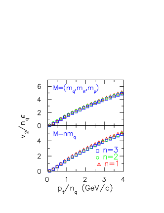
Figure 4: Scaled values for elliptic flow as a function of scaled transverse momentum for coalesced composite objects of $n_{q}=1,2,3$ quarks in the hydrodynamically inspired blast-wave model. Lower panel: Composite objects have masses $M_{C}=n_{q}m_{q}$ with a constituent quark mass of $m_{q}=350$ MeV. Upper panel: Composite objects have masses $m_{q}$, pion mass, proton mass for $n_{q}=1,2,3$ respectively. The values of $v_{2}$ are affected very little for $p_{t}/n_{q}\geq 1$ GeV/c.

In order to understand the degree to which mass effect destroy the scaling of $v_{2}$ with quark-number, we repeated the calculations of the previous subsection for the hydrodynamically inspired blast-wave model. Instead of using hadronic masses equal to $M_{c}=350n_{q}$ MeV, we use the pion mass for the two quark state and the proton mass for the three quark state. The comparison of the two choices for masses is displayed in Fig. 4. Remarkably little variation is observed for the different curves. We also found no observable changes for the shell-profile blast-wave calculations with similar mass modifications (not shown here). A significant sensitivity to the mass is however observed if one focuses at low $p_{t}$ below 500 MeV/c. The sensitivity is also more apparent for lower collective velocities.

The third criteria for implementation of the thermal expression, i.e. the addition of chemical potentials, implicitly requires that there are conserved charges or numbers with $Q_{C}=Q_{a}+Q_{b}$. If quark number is conserved in the hadronization process, the chemical potential can be associated with the net number of quarks and anti-quarks. This is analogous to the implicit assumption in coalescence that the quark content is unaltered by hadronization. Whereas this assumption is certainly reasonable for the coalescence of protons into deuterons, it can be questionable for the case of quark coalescence since quark anti-quark pairs can be copiously created in hadronization as expected either from entropy arguments or from dynamic pictures that involve string breaking. However, for high $p_{t}$ mesons, it does seem reasonable to neglect fragmentation processes, since such processes involve a color flux tube to form between the outgoing quark and the thermal medium. This flux tube lowers the momentum of the outgoing quark by roughly one unit, and in an exponential spectrum, can be neglected at values of $p_{t}$ well above the temperature. The breaking of such strings should be important for observables concerning particles with $p_{t}<1.0$ GeV/c. One can make strong arguments that hadronization for quarks below 1 GeV is of much different character than the hadronization at higher values muellergroup .

IV Microscopic Simulations

More sophisticated models of heavy ion collisions, such as hydrodynamic or Boltzmann descriptions, provide more complicated forms for the final phase space density. By analyzing the results of these numerical models, one can gain insight into the validity of the assumptions of blast-wave parameterizations. Unfortunately, there is not yet a “standard model” for the evolution of a RHIC collision. Hydrodynamic models using equations-of-state based on lattice gauge theory tend to significantly over-predict the lifetime of the collision starcor ; phenixcor ; Heinz . Boltzmann approaches which effectively represent stiff equations of state tend to somewhat under-predict source sizes molnarhbt . Since the issue of the space-time development of the collision remains uncertain at the 50% level, we will instead focus on a simplified Boltzmann description. By adjusting the cross sections and the initial conditions, we intend to better understand how and why $v_{2}(y_{t})$ can depend on $n_{q}$.

For the first calculation, we consider a system of 500 constituent quarks per unit rapidity of mass 350 MeV and initially thermalized at a temperature of 275 MeV. The particles are then allowed to collide with simple s-wave cross sections using the code GROMIT gromit to solve the Boltzmann equation. The initial density distribution in the transverse directions are set by either a Gaussian distribution, or by an ellipse with constant density. The initial sizes for the Gaussian profiles are chosen to be $R_{x}=2$ fm and $R_{y}=2.6$ fm, while for the ellipse, the radii are 4 and 5.2 fm. The longitudinal distributions are initialized according to boost invariant criteria, $v_{z}=z/t$. Boost-invariant constraints are maintained by cyclic boundary conditions along the $z$ axis.

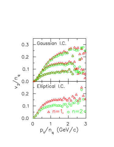
Figure 5: Scaled values for elliptic flow $v_{2}/n_{q}$ as a function of scaled transverse momentum $p_{t}/n_{q}$ from Boltzmann transport calculation. Upper panel: The initial state evolved from Gaussian density profile with elastic scattering cross sections of $\sigma=5,20$ and 80 mb (bottom to up). Nearly perfect scaling with quark number is exhibited. Lower panel: The initial state evolved from elliptic density profile with a sharp cutoff. $v_{2}$ significantly violate quark-number scaling.

The upper panel of Fig. 5 shows calculated values of $v_{2}$ from simulations using three cross sections, 5 mb, 20 mb and 80 mb. In addition to the $v_{2}$ for constituent quarks ($n_{q}=1$), $v_{2}$ for coalesced mesons ($n_{q}=2$) are also shown. Meson coalescence is calculated by sorting the quarks into bins according to their transverse momentum $p_{t}$ and azimuthal angle $\phi_{p}$, then coalescing them with a weight proportional to $\exp(-\delta r^{2}/2r_{c}^{2})$, where $\delta r$ is the separation of the two quarks as measured in the two-particle rest frame. The coalescence distance $r_{c}$ is chosen to be 1 fm. Constituent number scaling appears to be satisfied to high precision for all three cross sections. This is probably due to the fact that the initial conditions and equation of state satisfy the conditions for the scaling hydrodynamic solution discussed in the previous section, which in the limit of small flow velocities can be shown to lead to quark-number scaling.

Calculations based on an initial elliptic profile with sharp cutoff are displayed in the lower panel of Fig. 5. Aside from the density profile, the calculation was the same as was shown for the Gaussian profile with a cross section of 20 mb. In this case, quark-number scaling is significantly violated. This failure can be attributed to the shock wave which develops from the discontinuity in the density. From the perspective of hydrodynamics, there is no pressure gradient except at the surface. This forces the development of a shock wave. Emission is then more surface-like and less volume-like, which is more suggestive of the illustration on the right hand side of Fig. 1. For surface-like emission, one expects the asymmetry to owe itself to the disparity in the effective surface areas for emitting in- and out-of-plane, rather than to asymmetries in the respective phase space densities. For equations of state that incorporate a large latent heat, shock waves also develop since there is a large region of mixed phase for which there is no pressure gradient and therefore no transverse acceleration GulMat ; Rischke . One may also expect to observe violations from scaling in these instances. It will be interesting to analyze hydrodynamic calculations to see whether the presence of a large latent heat will, indeed, manifest itself in the behavior of $v_{2}$.

V Summary

Quark-number scaling for elliptic flow has been advocated as a signal for quark recombination. The two principal goals of this study are to identify precise conditions for quark number scaling, and to determine the degree to which thermal, coalescence, and microscopic models may realize these conditions.

Two conditions are necessary for realizing quark-number scaling. First, the phase space density for a composite object must equal the product of the phase space densities of the constituent quarks. Second, the effective volume for quarks that have a given momentum must be independent of azimuthal direction. It will be much more difficult to determine the validity of the latter condition since the effective volume is determined both by details of the spatial source size and by the collective flow and temperature.

The requirement of factorization is manifestly satisfied by coalescence models. It is approximately satisfied by thermal models, and becomes exactly satisfied in the limit that the masses of the coalesced hadron equal the product of $n_{q}$ and the constituent quark mass. However, we never observe a significant dependence to the behavior of $v_{2}$ as we varied the masses of the final hadrons for $p_{t}/n_{q}$ ¿ 1 GeV/c, the range of interest for quark recombination arguments. It should be emphasized, that in a thermal model, the only means to have non-uniform densities are by varying the temperature and chemical potential. If non-uniform chemical potentials are responsible for the density profile, thermal models implicitly assume that charge must be conserved by hadronization. For the hydrodynamically inspired blast-wave with a Gaussian profile, the temperature is kept constant, and the density is driven by non-uniformities in the chemical potential. Quark-number scaling for this model is then dependent on the baryons having 3/2 the charge of a meson, although this sensitivity is weak due to the linearity of $v_{2}$ vs. $p_{t}$.

The models invoked in this study are schematic by nature, but they provide several important informations regarding the interplay of coalescence and elliptic flow. It does appear that linear velocity profiles with sudden time-like break-up surfaces promote constituent-number scaling criteria of Eq. (2). This is verified by both blast-wave and microscopic modeling. Since linear velocity profiles tend to develop, except in the presence of strong shocks, Eq. (2) should be valid unless the initial density profile is abnormally sharp, or if the equation of state has a strong first-order phase transition.

Furthermore, the scaling condition can be tested by measuring the source-size as a function of the azimuthal volume. This can be done either with correlations or with coalescence ratios. If the source-size volumes at a given $p_{t}$ are independent of the azimuthal angle, it follows that constituent-number scaling of $v_{2}$ should be satisfied if the factorization criteria are met. Perhaps the easiest way to test this will be to estimate the $d/p^{2}$ ratio for deuterons and protons at the same transverse rapidity. This ratio is inversely proportional to the source size volume, so if constituent-number scaling is valid, it should be independent of the azimuthal angle. In other words, the $v_{2}$ for deuterons will then be twice $v_{2}$ for protons.

We have explored numerous models for the satisfaction of quark-number scaling:

1. Four different distortions of a blast-wave with an elliptic-shell geometry.

2. The blast-wave model of Retiere and Lisa, with both in-plane and out-of-plane extended profiles.

3. A blast-wave with simple linear behavior for the collective velocity and either a Gaussian or sharp elliptic profiles for the density.

4. A solution of the Boltzmann transport equation with a coalescence prescription for combining quarks into hadrons. Both Gaussian and sharp elliptic profiles are used for the initial densities.

In each of these prescriptions, the factorization condition is explicitly satisfied. Thus, the satisfaction of quark-number scaling depend solely on whether the effective volumes are $\phi$-independent. Unfortunately, it is not algebraically possible to show that any of the models explicitly satisfy quark-number scaling, except for the blast-wave with linear velocity gradients and a Gaussian profile in the limit of small expansion velocities and non-relativistic temperatures. However, an empirical pattern does seems to emerge: Linear velocity gradients and sudden volume-like disintegrations seem to closely satisfy quark-number scaling. Hydrodynamic evolutions tend to approach this geometry, except in the case of surface-like emission, which will be favored if shock waves are to develop. Shock waves are expected if the initial density has a sharp fall-off, or if there is a large latent heat which will lower the interior pressure of the fireball to give a shock wave the opportunity to develop.

Quark recombination is synonymous with satisfaction of the first condition, factorization of the phase space density of the combined object. This is because factorization assumes that two-particle densities are products of single-particle densities, i.e., jet-like correlations are lost. However, since factorization represents only one of the two conditions for quark-number scaling of $v_{2}$, there is always some ambiguity in concluding that both conditions are satisfied when one observes the scaling. For instance, it could be that neither condition is satisfied, but that the failures to meet both conditions conspired in some way to mimic the satisfaction of both criteria. Of course, a stronger case can be made if scaling is observed for a large number of cases. However, one must also remember that if the various cases involve hadrons with different cross sections, i.e., strange vs. non-strange hadrons, then one may expect violations of $v_{2}$. This can be understood by viewing Fig. 5 where the overall value of $v_{2}$ is shown to be strongly sensitive to the cross section.

Our investigations of both model results and of the underlying theory shows that observing quark-number scaling of $v_{2}$ indeed suggests that quark recombination may be at hand, but there are quite a large number of caveats that prevent one from declaring this as a stand-alone signature. However, it is clear that $v_{2}$ is, at the very least, very sensitive to the evolution, break-up mechanism and hadronization of the fire-ball. Thus, the details of the behavior of $v_{2}$ can be used to disqualify a large number of potential models, even if pointing to the root cause of the disqualifying attributes might be somewhat ambiguous.

We conclude by recommending that source-size measurements at intermediate $p_{t}$ can significantly clarify some of the issues surrounding quark recombination. First, interferometric or coalescence measurements may determine the source size as a function of $p_{t}$ and $\phi$. If source sizes are seen to be independent of the azimuthal angle, it should support the statement that quark-number scaling demonstrates that phase space densities factorize. More importantly, a simpler and more direct point can be made about such source-size measurements. If all particles in the intermediate-$p_{t}$ region with the same azimuthal angle originate from the same jet, the source size from correlation or coalescence analyses will be identical to that expected from $pp$ collisions of $\sim 1$ fm. If the emissions are independent, and factorization is valid, the source sizes will reflect the entire emitting region of such particles. Even if emission of high energy particles is confined to the surface during the first few fm/c, the effective volumes will be on the order of tens of cubic fm. The real value probably lies somewhere in between. Since jet-like correlations are observed at these $p_{t}$ region expjetcorrelations , the assumption of completely independent sources is probably not viable and more detailed models which incorporate jet-like correlations into coalescence pictures are currently being developed friesjetcorrelations ; molnar2004 . A measurement of the source volume will then provide crucial quantitative information to decide the relative role of recombination.

- (1) K. Adcox, et al., Phys. Rev. Lett. 88, 242301 (2002); Phys. Rev. Lett. 88, 022301 (2002).
- (2) S.A. Voloshin, Nucl. Phys. A715, 379 (2003).
- (3) R.J. Fries, B. Müller, C. Nonaka and S.A. Bass, Phys. Rev. Lett. 90, 202303 (2003).
- (4) V. Greco, C.M. Ko and P. Levai, Phys.Rev. C 68, 034904 (2003); Phys. Rev. Lett. 90, 202302 (2003).
- (5) R.J. Fries, B. Müller, C. Nonaka, S.A. Bass, Phys. Rev. C 68, 044902 (2003); C. Nonaka, R.J. Fries and S.A. Bass., Phys. Lett. B583, 73 (2004); C. Nonaka, B. Müller, M. Asakawa, S.A. Bass and R.J. Fries, Phys.Rev. C 69, 031902 (C) (2004).
- (6) D. Molnár and S.A. Voloshin, Phys. Rev. Lett. 91, 092301 (2003).
- (7) J.-Y. Ollitrault, Phys. Rev. D 46, 229 (1992).
- (8) S.A. Voloshin and Y. Zhang, Z. Phys. C70, 665 (1996).
- (9) K. Schweda [STAR Collaboration], ArXiv.org:nucl-ex/0403032 (2004); M. Kaneta [PHENIX Collaboration], ArXiv.org:nucl-ex/0404014; J. Adams et al., Phys. Rev. Lett. 92, 052302 (2004); S. Adler et al., Phys. Rev. Lett. 91, 182301 (2003).
- (10) E. Schnedermann, J. Sollfrank, and U. Heinz, Phys. Rev. C 48, 2462 (1993).
- (11) P. Huovinen, P.F. Kolb, U. Heinz, P.V. Ruuskanen, and S. Voloshin, Phys. Lett. B503, 58 (2001).
- (12) S.V. Akkelin, T. Csörgő, B. Lukács, Yu.M. Sinyukov and M. Weiner, Phys. Lett. B505, 64 (2001); M. Csanad, T. Csörgő, B. Lorstad and A. Ster, ArXiv.org:nucl-th/0402036; T. Csörgő, F. Grassi, Y. Hama, T. Kodama, Phys. Lett. B565, 107 (2003).
- (13) F. Retiere and M. Lisa, ArXiv.org:nucl-th/0312024.
- (14) A. Schwarzschild and C̆. Zupanc̆ic̆, Phys. Rev. 129, 854 (1963).
- (15) M. Gyulassy, K. Frankel, and E.A. Remler, Nucl. Phys. A402, 596 (1983).
- (16) P. Danielewicz and G.F. Bertsch, Nucl. Phys. A533, 712 (1991).
- (17) J.L. Nagle, B.S. Kumar, D. Kusnezov, H. Sorge, and R. Mattiello, Phys. Rev. C 53, 367 (1996).
- (18) D.E. Kahana, S.H. Kahana, Y. Pang, A.J. Baltz, C.B. Dover, E. Schnedermann, and T.J. Schlagel, Phys. Rev. C 54, 338 (1996).
- (19) R. Mattiello, H. Sorge, H. Stöcker, and W. Greiner, Phys. Rev. C 55, 1443 (1997).
- (20) J. Schaffner-Bielich, R. Mattiello, and H. Sorge, Phys. Rev. Lett. 84, 4305 (2000).
- (21) A. Mekjian, Phys. Rev. Lett. 38, 640 (1977).
- (22) W.J. Llope et al., Phys. Rev. C 52, 2004 (1995).
- (23) S. Pratt, Phys. Rev. C 56, 1095 (1997).
- (24) Q.H. Zhang, U.A. Wiedemann, C. Slotta and U.W. Heinz, Phys. Lett. B407, 33 (1997).
- (25) C. Adler, et al., Phys. Rev. Lett. 87, 082301 (2001).
- (26) K. Adcox, et al., Phys. Rev. Lett. 88, 192302 (2002).
- (27) M. Lisa [STAR Collaboration], Acta Phys. Polon. B35, 37 (2004).
- (28) C. Adler, et al., Phys. Rev. Lett. 87, 262301 (2001).
- (29) S. Pal and S. Pratt, Phys. Lett. B578, 310 (2004).
- (30) M. Gyulassy and T. Matsui, Phys. Rev. D 29, 419 (1984).
- (31) D.H. Rischke and M. Gyulassy, Nucl. Phys. A597, 701 (1996); Nucl. Phys. A608, 479 (1996).
- (32) D. Molnár, ArXiv.org:nucl-th/0408044.
- (33) U.W. Heinz and P.F. Kolb, Nucl. Phys. A702, 269 (2002); hep-ph/0204061.
- (34) D. Molnar and M. Gyulassy, Phys.Rev.Lett. 92, 052301 (2004).
- (35) S. Cheng, S. Pratt, P. Csizmadia, Y. Nara, D. Molnar, M. Gyulassy, S.E. Vance and B. Zhang, Phys. Rev. C 65, 024901 (2002).
- (36) C. Adler, et al., Phys. Rev. Lett. 90, 082302 (2003); A. Sickles, ArXiv.org:nucl-ex/0403028.
- (37) R.J. Fries, S.A. Bass and B. Müller, ArXiv.org:nucl-th/0407102 (2004).
- (38) D. Molnár, Acta Phys. Hung. A19, 1 (2004).