Description of nuclear octupole and quadrupole deformation close to the axial symmetry and phase transitions in the octupole mode

Abstract

The dynamics of nuclear collective motion is investigated in the case of reflection-asymmetric shapes. The model is based on a new parameterization of the octupole and quadrupole degrees of freedom, valid for nuclei close to the axial symmetry. Amplitudes of oscillation in other degrees of freedom different from the axial ones are assumed to be small, but not frozen to zero. The case of nuclei which already possess a permanent quadrupole deformation is discussed in some more detail and a simple solution is obtained at the critical point of the phase transition between harmonic octupole oscillation and a permanent asymmetric shape. The results are compared with experimental data of the Thorium isotopic chain. The isotope ²²⁶Th is found to be close to the critical point.

I Introduction

Phase transitions in nuclear shapes have been recently observed at the boundary between regions characterized by different intrinsic shapes of quadrupole deformation. It has been shown by Iachello Iachello (2000a, b, 2001) that new dynamic symmetries, called E(5), X(5) and Y(5) hold, respectively, at the critical point between spherical shape and $\gamma$–unstable deformation, between spherical and deformed axially symmetric shape and between deformed axial and triaxial shape. Here, we are mainly interested in the second case. First examples of X(5) symmetry in transitional nuclei have been found in ¹⁵²Sm Casten and Zamfir (2001) and ¹⁵⁰Nd Krucken et al. (2002). Other candidates for the X(5) symmetry in different nuclear regions have been reported later Bizzeti and Bizzeti-Sona (2002); Hutter et al. (2003); Clark et al. (2003); Fransen et al. (2004); Bizzeti (2003); Bijker et al. (2003, 2004); Tonev et al. (2004). From the theoretical point of view, slightly different potentials have been explored by Caprio Caprio (2004) and by Bonatsos et al. Bonatsos et al. (2004), while the evolution of the $s=2$ band when the lower border of the square well potential is displaced from zero has been investigated by Pietralla and Gorbachenko Pietralla and Gorbachenko (2004).

A similar phase transition (i.e., from shape oscillation to permanent deformation, conserving the axial symmetry of the system) could take place also in the octupole degree of freedom. We have found a possible example of such a phase transition in the Thorium isotope chain, with the critical point close to the mass 226. In this case, the octupole mode is combined with a stable quadrupole deformation. Preliminary results have been reported in two recent Conferences Bizzeti and Bizzeti-Sona (2004); Bizzeti (2003).

In order to provide a theoretical frame where to discuss the different aspects of the octupole motion, we introduce a new parameterization of the quadrupole and octupole degrees of freedom, valid in conditions close to the axial symmetry. In this limit, a model similar to the classical one by Bohr Bohr (1952) has been developed. This is the subject of the first part of this paper. In the second part, the model is used to discuss the evolution of the octupole mode along the isotopic chain of Thorium, and the results are compared with the experimental data.

II Theoretical frame for combined quadrupole and octupole excitations

II.1 Previous investigations of the Octupole plus Quadrupole deformation

Reflection–asymmetric nuclear shapes have been discussed in a number of papers, either in terms of surface Quadrupole + Octupole deformation (Bohr geometrical approach) or with an extended Interacting Boson Model (algebraic approach). The latter, proposed in 1985 by Engel and Iachello Engel and Iachello (1985), has been recently used by Alonso et al. Alonso et al. (1995), Raduta et al. Raduta and Ionescu (2003); Raduta et al. (1996a), Zamfir and Kusnezov Zamfir and Kusnezov (2001, 2003). An alternative approach assuming $\alpha$–cluster configurations has been discussed by Shneidman et al. Shneidman et al. (2002). In the frame of the geometrical approach, a number of theoretical investigations of the octupole vibrations around a stable quadrupole deformation have been reported in the last 50 years Rohozinski (1988); Butler and Nazarewicz (1996); Lipas and Davidson (1961); Denisov and Dzyublik (1995); Jolos and von Brentano (1999); Minkov et al. (2000, 2004). Most of them, however, are limited to the case of axial symmetry. This approach has been criticized, e.g., by Donner and Greiner Donner and Greiner (1966), who have stressed the fact that all terms of a given tensor order must be taken into account for a consistent treatment. To do this, Donner and Greiner renounce to the use of an “intrinsic frame” referred to the principal axes of the overall tensor of inertia and choose to define the octupole amplitudes in the “intrinsic frame” of the quadrupole mode alone. In this approach, definite predictions have been obtained at the limit where the octupole deformations are “small” in comparison with the quadrupole ones Eisenberg and Greiner (1987).

II.2 The new parameterization

Here we adopt a different approach, which can be useful also in the case of comparable octupole and quadrupole deformation, close to the axial–symmetry limit. Namely, we choose as “intrinsic” reference frame the principal axes of the overall tensor of inertia, as it results from the combined quadrupole and octupole deformation. The definitions of quadrupole and octupole amplitudes $a^{(\lambda)}_{\mu}$, with $\lambda=2,3$ and $a^{(\lambda)}_{-\mu}=(-)^{\mu}\ {a^{(\lambda)}_{\mu}}^{*}$, are recalled in the Appendix A. All these amplitudes are defined in the (non inertial) intrinsic frame. To this purpose, in the case of the quadrupole mode alone, it is enough to assume $a^{(2)}_{2}\!=a\!^{(2)}_{-2}$ real and $a^{(2)}_{\pm 1}\!=\!0$, with the standard parameterization in terms of $\beta_{2}$ and $\gamma_{2}$:

$$a^{(2)}_{0} = \beta_{2}\cos\gamma_{2}$$ (1a)

$$a^{(2)}_{1} = 0$$ (1b)

$$a^{(2)}_{2} = \sqrt{1/2}\ \beta_{2}\ \sin\gamma_{2}\ .$$ (1c)

For the octupole mode alone, a parameterization suitable to this purpose has been proposed in 1999 by Wexler and Dussel Wexler and Dussel (1999). We adopt here a very similar one:

$$a^{(3)}_{0} = \beta_{3}\ \cos\gamma_{3}$$ (2a)

$$a^{(3)}_{1} = -(5/2)\ \left(X+iY\right)\ \sin\gamma_{3}$$ (2b)

$$a^{(3)}_{2} = \sqrt{1/2}\ \beta_{3}\ \sin\gamma_{3}$$ (2c)

$$a^{(3)}_{3} = X\left[\cos\gamma_{3}+(\sqrt{15}/2)\ \sin\gamma_{3}\right]$$ (2d)

$$+ i\ Y\left[\cos\gamma_{3}-(\sqrt{15}/2)\ \sin\gamma_{3}\right]\ .$$

With this choice, the tensor of inertia turns out to be diagonal (see Appendix A).

In both cases, one has to consider, in addition to the intrinsic variables ($\beta_{2},\ \gamma_{2}$ for the quadrupole, or $\beta_{3},\ \gamma_{3}\ ,X\ ,Y$ for the octupole), the three Euler angles defining the orientation of the intrinsic frame in the laboratory frame, in order to reach a number of parameters equal to the number of degrees of freedom (5 for the quadrupole, 7 for the octupole).

Unfortunately, the situation is not so simple when quadrupole and octupole modes are considered together, as the intrinsic frames of the two modes do not necessarily coincide. We shall limit our discussion to situations close to the axial symmetry limit – in which, obviously, the two frames coincide – and define a parametrization which automatically sets to zero the three products of inertia $\mathcal{J}_{\kappa,\kappa^{\prime}}$ ($\kappa\neq\kappa^{\prime}$) up to the first order in the amplitudes of non–axial modes.

To this purpose we put

$$a^{(\lambda)}_{\mu}=\bar{a}^{(\lambda)}_{\mu}+\tilde{a}^{(\lambda)}_{\mu}$$ (3)

where $\bar{a}^{(\lambda)}_{\mu}$ are defined according to the eq.s (1,2) and $\tilde{a}^{(\lambda)}_{\mu}$ are correction terms, which are assumed to be small compared to the axial amplitudes $a^{(\lambda)}_{0}$, but of the same order of magnitude as the other non-axial terms. It will be enough to consider these corrections only for those amplitudes which, according to eq.s (1,2), are either zero or small of the second order: the imaginary part of $a^{(2)}_{2},\ a^{(3)}_{2}$ and the real and imaginary parts of $a^{(2)}_{1},\ a^{(3)}_{1}$. The six “new” first–order amplitudes added to those of eq.s (1,2) are, however, not independent from one another, if we choose as the reference systeme the one in which the three products of inertia turn out to be zero.

The expressions of the inertia tensor as a function of the deformation parameters, obtained with the Bohr assumptions Bohr (1952) of not–too–big deformations and irrotational flow, are given in the Appendix A. In order to simplify the notations, from now on we consider the inertia parameters $B_{2},\ B_{3}$ included in our definitions of the amplitudes $a^{(\lambda)}_{\mu}$, which therefore correspond to $\sqrt{B_{\lambda}}\ a^{(\lambda)}_{\mu}$ in the original Bohr notations. From the eq.s (58), and retaining only terms of the first order in the small amplitudes $a^{(\lambda)}_{\mu}$ with $\mu\neq 0$, we obtain the conditions

$$\mathcal{J}_{12} = -2\sqrt{6}\left(\beta_{2}{\rm Im}\ \tilde{a}^{(2)}_{2}+\sqrt{5}\beta_{3}{\rm Im}\ \tilde{a}^{(3)}_{2}\right)=0$$ (4a)

$$\mathcal{J}_{13} + i\mathcal{J}_{23}\ =\ \sqrt{6}\ \left(\beta_{2}\tilde{a}^{(2)}_{1}+\sqrt{2}\beta_{3}\tilde{a}^{(3)}_{1}\right)=0$$ (4b)

which are satisfied (at the leading order) if we put

$$\begin{array}[c]{lp{0.1mm}lp{0mm}l}\tilde{a}^{(2)}_{1}=\!\frac{-\sqrt{2}\beta_{3}}{\sqrt{\beta_{2}^{2}+2\beta_{3}^{2}}}\left(\eta+i\zeta\right)&&\tilde{a}^{(3)}_{1}=\!\frac{\beta_{2}}{\sqrt{\beta_{2}^{2}+2\beta_{3}^{2}}}\left(\eta+i\zeta\right)\\[8.0pt] {\rm Im}\;\tilde{a}^{(2)}_{2}=\!\frac{-\sqrt{5}\beta_{3}}{\sqrt{\beta_{2}^{2}+5\beta_{3}^{2}}}\xi&&{\rm Im}\;\tilde{a}^{(3)}_{2}=\!\frac{\beta_{2}}{\sqrt{\beta_{2}^{2}+5\beta_{3}^{2}}}\xi\end{array}$$ (5)

with the new parameters $\eta,\ \zeta$ and $\xi$ small of the first order. It is clear that only the ratios of the relevant amplitudes are constrained by the eq.s (4). The definition of the new variables given in each line of eq.s (5) contain therefore an arbitrary factor. Our choice (and in particular for the square–root factors at the denominators) has some distinguished advantage, which will result clear from the classical expression of the kinetic energy, discussed in the next paragraph.

In the intrinsic reference frame, and at the same order of approximation, the values of the three principal moments of inertia can be derived from eq.s (56,57):

$$\mathcal{J}_{1} = 3(\beta_{2}^{2}+2\beta_{3}^{2})+2\sqrt{3}(\beta_{2}^{2}\gamma_{2}+\sqrt{5}\beta_{3}^{2}\gamma_{3})$$ (6a)

$$\mathcal{J}_{2} = 3(\beta_{2}^{2}+2\beta_{3}^{2})-2\sqrt{3}(\beta_{2}^{2}\gamma_{2}+\sqrt{5}\beta_{3}^{2}\gamma_{3})$$ (6b)

$$\mathcal{J}_{3} = 4(\beta_{2}^{2}\gamma_{2}^{2}+\beta_{3}^{2}\gamma_{3}^{2})+18(X^{2}+Y^{2})$$ (6c)

$$+2(\eta^{2}+\zeta^{2})+8\xi^{2}\ .$$

With the amplitudes given by eq.s (1,2) the principal axes of the quadrupole would coincide with those of the octupole. It is not necessarily so with our more general assumptions. When $a^{(\lambda)}_{1}\neq 0$, the axis 3 of the tensor of inertia for the quadrupole mode alone does not coincide with that of the octupole. If $a^{(\lambda)}_{1}=0$, but Im$\ a^{(\lambda)}_{2}\neq 0$, the misalignment concerns the other two principal axes perpendicular to the common axis 3.

Table 1: The matrix of inertia $\mathcal{G}$: leading terms and relevant first-order terms. Other first-order terms are indicated with the symbol $\approx 0$. As the matrix is symmetric, first-order terms in the last three columns are not explicitly shown. Here $\mathcal{J}_{1}=3(\beta_{2}^{2}+2\beta_{3}^{2})+2\sqrt{3}(\beta_{2}^{2}\gamma_{2}+\sqrt{5}\beta_{3}^{2}\gamma_{3})$; $\mathcal{J}_{2}=3(\beta_{2}^{2}+2\beta_{3}^{2})-2\sqrt{3}(\beta_{2}^{2}\gamma_{2}+\sqrt{5}\beta_{3}^{2}\gamma_{3})$ ; and $\mathcal{J}_{3}=4(\beta_{2}^{2}\gamma_{2}^{2}+\beta_{3}^{2}\gamma_{3}^{2})+18(X^{2}+Y^{2})+2(\eta^{2}+\zeta^{2})+8\xi^{2}$.
The determinant of the matrix is  ${G={\rm Det}\mathcal{G}=1152\beta_{2}^{2}\beta_{3}^{2}\big{(}\beta_{2}^{2}+2\beta_{3}^{2}\big{)}^{2}\big{(}\beta_{2}^{2}+5\beta_{3}^{2}\big{)}^{-1}\big{(}\beta_{2}^{2}\gamma_{2}+\sqrt{5}\ \beta_{3}^{2}\gamma_{3}\big{)}^{2}}$.

	$\dot{\beta_{2}}$	$\dot{\gamma_{2}}$	$\dot{\beta_{3}}$	$\dot{\gamma_{3}}$	$\dot{X}$	$\dot{Y}$	$\dot{\xi}$	$\dot{\eta}$	$\dot{\zeta}$	$q_{1}$	$q_{2}$	$q_{3}$
$\dot{\beta_{2}}$	1	0	0	0	0	0	0	0	0	$\left[..\right]$	$\left[..\right]$	0
$\dot{\gamma_{2}}$	0	$\beta_{2}^{2}$	0	0	0	0	0	0	0	$\left[..\right]$	$\left[..\right]$	$(..)$
$\dot{\beta}_{3}$	0	0	1	0	0	0	0	0	0	$\left[..\right]$	$\left[..\right]$	0
$\dot{\gamma_{3}}$	0	0	0	$\beta_{3}^{2}$	$\left[\sqrt{15}X\right]$	$\left[-\!\sqrt{15}Y\right]$	0	$\left[-\frac{5\beta_{2}X}{\sqrt{\beta_{2}^{2}+2\beta_{3}^{2}}}\right]$	$\left[-\frac{5\beta_{2}Y}{\sqrt{\beta_{2}^{2}+2\beta_{3}^{2}}}\right]$	$\left[..\right]$	$\left[..\right]$	$(..)$
$\dot{X}$	0	0	0	$\left[\sqrt{15}X\right]$	$2\!+\!2\sqrt{15}\gamma_{3}$	0	0	$\left[-\frac{5\beta_{2}\gamma_{3}}{\sqrt{\beta_{2}^{2}+2\beta_{3}^{2}}}\right]$	0	$\left[..\right]$	$\left[..\right]$	$(..)$
$\dot{Y}$	0	0	0	$\left[-\!\sqrt{15}Y\right]$	0	$2\!-\!2\sqrt{15}\gamma_{3}$	0	0	$\left[-\frac{5\beta_{2}\gamma_{3}}{\sqrt{\beta_{2}^{2}+2\beta_{3}^{2}}}\right]$	$\left[..\right]$	$\left[..\right]$	$(..)$
$\dot{\xi}$	0	0	0	0	0	0	2	0	0	$\left[..\right]$	$\left[..\right]$	$(..)$
$\dot{\eta}$	0	0	0	$\left[-\frac{5\beta_{2}X}{\sqrt{\beta_{2}^{2}+2\beta_{3}^{2}}}\right]$	$\left[-\frac{5\beta_{2}\gamma_{3}}{\sqrt{\beta_{2}^{2}+2\beta_{3}^{2}}}\right]$	0	0	2	0	$\left[..\right]$	$\left[..\right]$	$(..)$
$\dot{\zeta}$	0	0	0	$\left[-\frac{5\beta_{2}Y}{\sqrt{\beta_{2}^{2}+2\beta_{3}^{2}}}\right]$	0	$\left[-\frac{5\beta_{2}\gamma_{3}}{\sqrt{\beta_{2}^{2}+2\beta_{3}^{2}}}\right]$	0	0	2	$\left[..\right]$	$\left[..\right]$	$(..)$
$q_{1}$	$\approx 0$	$\approx 0$	$\approx 0$	$\approx 0$	$\approx 0$	$\approx 0$	$\approx 0$	$\approx 0$	$\approx 0$	${\mathcal{J}_{1}}$	0	0
$q_{2}$	$\approx 0$	$\approx 0$	$\approx 0$	$\approx 0$	$\approx 0$	$\approx 0$	$\approx 0$	$\approx 0$	$\approx 0$	0	${\mathcal{J}_{2}}$	0
$q_{3}$	0	$\frac{-\!\sqrt{40}\beta_{2}\beta_{3}\xi}{\sqrt{\beta_{2}^{2}+5\beta_{3}^{2}}}$	0	$\frac{\sqrt{8}\beta_{2}\beta_{3}\xi}{\sqrt{\beta_{2}^{2}+5\beta_{3}^{2}}}$	$6Y$	$-\!6X$	$\frac{\sqrt{8}\beta_{2}\beta_{3}(\sqrt{5}\gamma_{2}\!-\!\gamma_{3})}{\sqrt{\beta_{2}^{2}+5\beta_{3}^{2}}}\phantom{.}$	$2\zeta$.	$-2\eta$	0	0	$\mathcal{J}_{3}$

II.3 The classical expression of the kinetic energy

Now it is possible to express the classical kinetic energy (as given by Bohr hydrodynamical model) in terms of the new variables and of the intrinsic components $q_{\kappa}$ of the angular velocity. The classical expression has the form

$$T=\frac{1}{2}\sum\dot{Q}_{\mu}\mathcal{G}_{\mu\nu}\dot{Q}_{\nu}$$ (7)

where $\dot{Q}\equiv\{\dot{\xi}_{1},\dot{\xi}_{2},...,\dot{\xi}_{9},q_{1},q_{2},q_{3}\}$, $\dot{\xi}_{\mu}\ (\mu=1,...,9)$ are the time derivative of the nine parameters we have just defined, and $q_{1},\ q_{2},\ q_{3}$ are the intrinsic components of the angular velocity of the intrinsic system with respect to an inertial frame. The elements of the matrix $\mathcal{G}$ (leading terms and relevant first-order terms) are shown in the Table 1.

The determinant $G={\rm Det}\ \mathcal{G}$ takes the form

$$G\propto\beta_{2}^{2}\beta_{3}^{2}\big{(}\beta_{2}^{2}+2\beta_{3}^{2}\big{)}^{2}\big{(}\beta_{2}^{2}+5\beta_{3}^{2}\big{)}^{-1}\big{(}\beta_{2}^{2}\gamma_{2}+\sqrt{5}\ \beta_{3}^{2}\gamma_{3}\big{)}^{2}$$

and, at the limit $\beta_{3}\ll\beta_{2}$, results to be proportional to $\beta_{2}^{8}$, and therefore consistent with that of the Bohr model for a pure quadrupole motion. This is a consequence of our choice of the normalization factors in the eq.s (5). This choice has other advantages: all the non diagonal terms involving the time derivatives of $\beta_{2}$ or $\beta_{3}$ and either the derivative of one of the other intrinsic amplitudes or $q_{3}$ turn out to be zero in the present approximation. Other non diagonal elements are small (of the first order) in the “small” amplitudes $\gamma_{2},\ \gamma_{3},\ X,\ Y,\ \xi,\ \eta,\ \zeta$. In situations close to the axial symmetry, they have negligible effect on the results (see Appendix B), with the only exception of elements of the last line and column. The latter, in fact, are still small of the first order, but must be compared with the diagonal element ${\mathcal{J}}_{3}$, which is small of the second order in the “small” non–axial amplitudes. These terms play an important role in the treatment of the intrinsic component of the angular momentum along the approximate axial–symmetry axis, which will be discussed in the next paragraph.

II.4 Intrinsic components of the angular momentum

According to the classical mechanics, the components $L_{1}$, $L_{2}$ and $L_{3}$ of the angular momentum in the intrinsic frame are obtained as the derivatives of the total kinetic energy with respect to the corresponding intrinsic component of the angular velocity:

$$L_{k}=\frac{\partial T}{\partial q_{k}}\ .$$ (8)

The part of the kinetic energy depending on the component $q_{k}$ has the form

$$T_{k}(q_{k})=\frac{1}{2}\mathcal{J}_{k}q_{k}^{2}+F_{k}q_{k}$$ (9)

where $F_{k}$ is a function of the dynamical variables $\xi_{i}$ and of their derivatives with respect to the time, and is small of the first order according to our definition. As for the moments of inertia, $\mathcal{J}_{3}$ is small of the second order, while $\mathcal{J}_{1}$, $\mathcal{J}_{2}$ are not small. According to eq.(8), we have

$$L_{k} = \mathcal{J}_{k}q_{k}+F_{k}$$

$$q_{k} = \frac{L_{k}-F_{k}}{\mathcal{J}_{k}}$$ (10)

$$T_{k}(L_{k}) = \frac{1}{2}\mathcal{J}_{k}\ \left[\frac{1}{\mathcal{J}_{k}}\big{(}L_{k}-F_{k}\big{)}\right]^{2}+F_{k}\left[\frac{1}{\mathcal{J}_{k}}\big{(}L_{k}-F_{k}\big{)}\right]$$ (11)

$$= \frac{L_{k}^{2}}{2\mathcal{J}_{k}}-\frac{F_{k}^{2}}{2\mathcal{J}_{k}}\ .$$

For $k=1,2$ the second term is small of the second order and can be neglected. It is not so for $k=3$, as $\mathcal{J}_{3}$ is also small and of the same order as $F_{k}^{2}$. In more detail, we have

$$L_{3} = \mathcal{J}_{3}q_{3}+\Big{[}\ \frac{\sqrt{8}\ \beta_{2}\beta_{3}}{\sqrt{\beta_{2}^{2}+5\beta_{3}^{2}}}\big{(}\gamma\dot{\xi}-\xi\dot{\gamma}\big{)}$$ (12)

$$+ 6\big{(}Y\dot{X}-X\dot{Y}\big{)}+2\big{(}\zeta\dot{\eta}-\eta\dot{\zeta}\big{)}\ \Big{]}$$

where we have put

$$\gamma=\sqrt{5}\ \gamma_{2}-\gamma_{3}\ .$$ (13)

At this point, it will be convenient to express the variables $\gamma_{2}$ and $\gamma_{3}$ as linear combinations of two new variables, one of which is, obviously, $\gamma=\sqrt{5}\gamma_{2}-\gamma_{3}$. The other one, that we call $\gamma_{0}$, can be chosen proportional to the linear combination which enters in the expression of the determinant $G$,

$$\gamma_{0}=c\left(\beta_{2}^{2}\gamma_{2}+\sqrt{5}\ \beta_{3}^{2}\gamma_{3}\right).$$ (14)

With this choice, we obtain

$$\gamma_{2} = \frac{\gamma_{0}/c+\sqrt{5}\ \beta_{3}^{2}\gamma}{\beta_{2}^{2}+5\beta_{3}^{2}}$$

$$\gamma_{3} = \frac{\sqrt{5}\ \gamma_{0}/c-\beta_{2}^{2}\gamma}{\beta_{2}^{2}+5\beta_{3}^{2}}$$ (15)

and, at the leading order,

$$\beta_{2}^{2}\dot{\gamma}_{2}^{2}+\beta_{3}^{2}\dot{\gamma}_{3}^{2}=\frac{\beta_{2}^{2}\beta_{3}^{2}}{\beta_{2}^{2}+5\beta_{3}^{2}}\dot{\gamma}^{2}+\frac{1}{\beta_{2}^{2}+5\beta_{3}^{2}}\ (\dot{\gamma}_{0}/c\big{)}^{2}\ .$$ (16)

In deriving the eq. 16, the factor $1/c$ has been considered constant. We may note,however, that the same result holds at the leading order also if $1/c$ is a function of $\beta_{2}$ and/or $\beta_{3}$. In fact, terms involving the time derivative of $1/c$ also contain the “small” quantity $\gamma_{0}$, and their effect is negligible in the present approximation (see Appendix B). E.g., one could choose for $1/c$ a quadratic expression in $\beta_{2},\ \beta_{3}$, in order to obtain for $\gamma_{0}$ an adimensional quantity, like $\gamma_{2},\ \gamma_{3}$ and $\gamma$. The same argument applies for possible redefinitions of other “small” variables, like $\gamma$.

The expression (12) can be somewhat simplified with the substitutions

$$X = w\sin\vartheta$$ (17a)

$$Y = w\cos\vartheta$$ (17b)

$$\eta = v\sin\varphi$$ (17c)

$$\zeta = v\cos\varphi$$ (17d)

$$\xi = u\sin\chi$$ (17e)

$$\gamma = \sqrt{2}\ \left(\sqrt{\beta_{2}^{2}+5\beta_{3}^{2}}\ /\ \beta_{2}\beta_{3}\right)u\cos\chi$$ (17f)

$$\frac{\gamma_{0}}{c} = f(\beta_{2},\beta_{3})\sqrt{\beta_{2}^{2}+5\beta_{3}^{2}}\ u_{0}$$ (17g)

which gives for the determinant of the matrix $\mathcal{G}$

$$G={\rm Det}\;\mathcal{G}=2304\big{(}\beta_{2}^{2}+2\beta_{3}^{2}\big{)}^{2}\ u_{0}^{2}\ v^{2}u^{2}w^{2}\ f^{2}(\beta_{2},\beta_{3}).$$ (18)

The choice of the function $f(\beta_{2},\beta_{3})$ is irrelevant for what concerns the angular momentum. Non diagonal terms (small of the first order) would depend on this choice, but their effect is negligible (see Appendix B). As a criterion to define the form of the function $f$, we observe that for permanent quadrupole deformation $\beta_{2}=\bar{\beta}_{2}$ and at the limit $\beta_{3}^{2}\ll\beta_{2}^{2}$ our value of $G$ must agree with the result given, at this limit, by Eisenberg and Greiner Eisenberg and Greiner (1987). This happens if the function $f$ we have left undetermined tends to a constant when $\beta_{2}\rightarrow\bar{\beta}_{2}$. We adopt here the simplest possible choice, i.e. $f(\beta_{2},\beta_{3})=1$, to obtain the matrix $\mathcal{G}$ given in the Table 2, and (at the leading order)

Table 2: The matrix of inertia $\mathcal{G}$ after the introduction of the new variables $u_{0}$, $v$, $u$, $w$, $\varphi$, $\chi$, and $\vartheta$ (see text). Here, $\mathcal{J}_{1}=\mathcal{J}_{2}=3(\beta_{2}^{2}+2\beta_{3}^{2})$, and $\mathcal{J}_{3}=4\ u_{0}^{2}+2v^{2}+8u^{2}+18w^{2}$. Only the leading terms are shown. Neglected terms are small of the first order (or smaller) in the sub-matrix involving only $\dot{\beta_{2}}$, $\dot{\beta_{3}}$, $\dot{u_{0}}$, $\dot{v}$, $\dot{u}$, $\dot{w}$, $q_{1}$ and $q_{2}$; of the third order (or smaller) in the sub-matrix involving only $\dot{\varphi}$, $\dot{\chi}$, $\dot{\vartheta}$ and $q_{3}$; of the second order (or smaller) in the rest of the matrix.

	$\dot{\beta_{2}}$	$\dot{\beta_{3}}$	$\dot{u_{0}}$	$\dot{v}$	$\dot{u}$	$\dot{w}$	$\dot{\varphi}$	$\dot{\chi}$	$\dot{\vartheta}$	$q_{1}$	$q_{2}$	$q_{3}$
$\dot{\beta_{2}}$	1	0	0	0	0	0	0	0	0	0	0	0
$\dot{\beta}_{3}$	0	1	0	0	0	0	0	0	0	0	0	0
$\dot{u_{0}}$	0	0	$1$	0	0	0	0	0	0	0	0	0
$\dot{v}$	0	0	0	2	0	0	0	0	0	0	0	0
$\dot{u}$	0	0	0	0	2	0	0	0	0	0	0	0
$\dot{w}$	0	0	0	0	0	2	0	0	0	0	0	0
$\dot{\varphi}$	0	0	0	0	0	0	$2v^{2}$	0	0	0	0	$2v^{2}$
$\dot{\chi}$	0	0	0	0	0	0	0	$2u^{2}$	0	0	0	$4u^{2}$
$\dot{\vartheta}$	0	0	0	0	0	0	0	0	$2w^{2}$	0	0	$6w^{2}$
$q_{1}$	0	0	0	0	0	0	0	0	0	$\mathcal{J}_{1}$	0	0
$q_{2}$	0	0	0	0	0	0	0	0	0	0	$\mathcal{J}_{2}$	0
$q_{3}$	0	0	0	0	0	0	$2v^{2}$	$4u^{2}$	$6w^{2}$	0	0	$\mathcal{J}_{3}$

$$G = {\rm Det}\;\mathcal{G}=2304\big{(}\beta_{2}^{2}+2\beta_{3}^{2}\big{)}^{2}\ u_{0}^{2}\ v^{2}u^{2}w^{2}$$ (19)

$$\mathcal{J}_{3} = 4u_{0}^{2}+2v^{2}+8u^{2}+18w^{2}$$ (20)

$$2T = \dot{\beta}_{2}^{2}+\dot{\beta}_{3}^{2}+\dot{u}_{0}^{2}$$ (21)

$$+ 2\big{(}\dot{v}^{2}+v^{2}\dot{\varphi}^{2}\big{)}+2\big{(}\dot{u}^{2}+u^{2}\dot{\chi}^{2}\big{)}+2\big{(}\dot{w}^{2}+w^{2}\dot{\vartheta}^{2}\big{)}$$

$$+ 2q_{3}\left[2v^{2}\dot{\varphi}+4u^{2}\dot{\chi}+6w^{2}\dot{\vartheta}\right]$$

$$+ \mathcal{J}_{1}q_{1}^{2}+\mathcal{J}_{2}q_{2}^{2}+\mathcal{J}_{3}q_{3}^{2}\ .$$

II.5 Classification of elementary excitations with respect to $K^{\pi}$

We can now deduce the intrinsic components of the angular momentum:

$$L_{1} = \mathcal{J}_{1}q_{1}$$ (22a)

$$L_{2} = \mathcal{J}_{2}q_{2}$$ (22b)

$$L_{3} = \mathcal{J}_{3}q_{3}+\left[2v^{2}\dot{\varphi}+4u^{2}\dot{\chi}+6w^{2}\dot{\vartheta}\right]$$ (22c)

$$= 2v^{2}\big{(}q_{3}+\dot{\varphi}\big{)}+4u^{2}\big{(}2q_{3}+\dot{\chi}\big{)}+6w^{2}\big{(}3q_{3}+\dot{\vartheta}\big{)}$$

$$+4u_{0}^{2}q_{3}\ .$$

In the same way, we can obtain the classical moments conjugate to $\chi$, $\vartheta$ and $\varphi$ (we observe that none of these variables appears in the expressions of $G$ or $\mathcal{J}_{3}$):

$$p_{\varphi} = 2v^{2}(\dot{\varphi}+q_{3})$$ (22d)

$$p_{\chi} = 2u^{2}\left(\dot{\chi}+2q_{3}\right)$$ (22e)

$$p_{\vartheta} = 2w^{2}(\dot{\vartheta}+3q_{3})\ .$$ (22f)

Now we can solve the system of equations (22) with respect to the variables $q_{1},\ q_{2},\ q_{3},\ \dot{\varphi},\ \dot{\chi},\ \dot{\vartheta}$. We obtain

$$q_{1} = L_{1}/\mathcal{J}_{1}$$ (23a)

$$q_{2} = L_{2}/\mathcal{J}_{2}$$ (23b)

$$q_{3} = \frac{1}{u_{0}}\big{(}L_{3}-p_{\varphi}-2p_{\chi}-3p_{\vartheta}\big{)}$$ (23c)

$$\dot{\varphi} = \frac{p_{\varphi}}{2v_{0}^{2}}-\frac{1}{u_{0}^{2}}\big{(}L_{3}-p_{\varphi}-2p_{\chi}-3p_{\vartheta}\big{)}$$ (23d)

$$\dot{\chi} = \frac{p_{\chi}}{2u^{2}}-\frac{2}{u_{0}^{2}}\big{(}L_{3}-p_{\varphi}-2p_{\chi}-3p_{\vartheta}\big{)}$$ (23e)

$$\dot{\vartheta} = \frac{p_{\vartheta}}{2\chi_{0}^{2}}-\frac{3}{u_{0}^{2}}\big{(}L_{3}-p_{\varphi}-2p_{\chi}-3p_{\vartheta}\big{)}$$ (23f)

The equations (23) have a very simple meaning in the case where the potential energy does not depend on the variables $\varphi$, $\chi$ or $\vartheta$. In such a case (a sort of model $\varphi$-$\chi$-$\vartheta$–instable, in the sense of the $\gamma$–instable model by Wilets and Jean Wilets and Jean (1956)) the conjugate moments of these three angular variables are constants of the motion, with integer eigenvalues $n_{\varphi}$, $n_{\chi}$ and $n_{\vartheta}$ (in units of $\hbar$). Moreover, if we assume that $u_{0}\rightarrow 0$, the third component $q_{3}$ of the angular velocity tends to $\infty$ unless $L_{3}-p_{\varphi}-2p_{\chi}-3p_{\vartheta}=0$ (eq. (23c)). In this case, the operator $L_{3}$ is diagonal, with eigenvalues $K=n_{\varphi}+2n_{\chi}+3n_{\vartheta}$, and the three degrees of freedom corresponding to $\varphi$, $\chi$ and $\vartheta$ can be associated to non-axial excitation modes with $K=$1, 2 and 3, respectively.

To investigate the character of the degree of freedom described by the parameter $u_{0}$, and for a deeper understanding of the nature of the other degrees of freedom, it is necessary to express the complete Hamiltonian in the frame of a definite model which, although not unique, is at least completely self-consistent at the limit close to the axial symmetry.

In fact, it is now possible to use the Pauli prescriptions Pauli (1933) to construct the quantum operator $\hat{T}$ corresponding to the classical kinetic energy $T$ of eq. (21). In doing this, we make use of the partial inversion of the matrix $\mathcal{G}$ given by the solution (23) of the linear system (22), and note that none of the variables $\varphi$, $\chi$, $\vartheta$ or $q_{3}$ enter in the expression of $G$:

$$\frac{2}{\hbar^{2}}\ \hat{T} = -\left\{\frac{1}{\beta_{2}^{2}+2\beta_{3}^{2}}\frac{\partial}{\partial\beta_{2}}\left[\big{(}\beta_{2}^{2}+2\beta_{3}^{2}\big{)}\frac{\partial}{\partial\beta_{2}}\right]\right.$$ (24)

$$+ \frac{1}{\beta_{2}^{2}+2\beta_{3}^{2}}\frac{\partial}{\partial\beta_{3}}\left[\big{(}\beta_{2}^{2}+2\beta_{3}^{2}\big{)}\frac{\partial}{\partial\beta_{3}}\right]$$

$$+ \frac{1}{u_{0}}\frac{\partial}{\partial u_{0}}\left[u_{0}\frac{\partial}{\partial u_{0}}\right]+\frac{1}{2v}\frac{\partial}{\partial v}\left[v\frac{\partial}{\partial v}\right]$$

$$+ \frac{1}{2u}\frac{\partial}{\partial u}\left[u\frac{\partial}{\partial u}\right]+\frac{1}{2w}\frac{\partial}{\partial w}\left[w\frac{\partial}{\partial w}\right]$$

$$+ \left.\ \frac{1}{2v^{2}}\frac{\partial^{2}}{\partial\varphi^{2}}+\frac{1}{2u^{2}}\frac{\partial 2}{\partial\chi 2}+\frac{1}{2w^{2}}\frac{\partial 2}{\partial\vartheta 2}\right\}$$

$$+ \frac{1}{4u_{0}^{2}}\ \left[\hat{L}_{3}-\frac{\partial}{\partial\varphi}-2\frac{\partial}{\partial\chi}-3\frac{\partial}{\partial\vartheta}\right]^{2}$$

$$+ \frac{1}{2\mathcal{J}_{1}}\ \hat{L}_{1}^{2}+\frac{1}{2\mathcal{J}_{2}}\ \hat{L}_{2}^{2}\ .$$

This is, admittedly, only a semi-classical discussion. However, the formal quantum treatment in the frame of the Pauli procedure, shown in the Appendix C, gives exactly the same result.

Until now, no assumption has been made on the form of the potential-energy operator, which will determine the particular model. A few general remarks on this subject are contained in the Appendix D. We now assume that the potential energy can be separated in the sum of a term depending only on $u_{0}$ and another containing the other dynamical variables. In this case the differential equation in the variable $u_{0}$ is approximately decoupled from the rest. One obtains the Schrödinger equation

$$\left\{\frac{1}{u_{0}}\frac{\partial}{\partial u_{0}}\left[u_{0}\frac{\partial}{\partial u_{0}}\right]\right. + \frac{2}{\hbar^{2}}\left[E_{u_{0}}-U(u_{0})\right]$$

$$-\ \frac{1}{u_{0}^{2}} \left.\left[\frac{\Omega_{u_{0}}}{2}\right]^{2}\right\}\phi(u_{0})=0$$ (25)

where we have put

$$\Omega_{u_{0}}=K-n_{\varphi}-2n_{\chi}-3n_{\vartheta}\ .$$ (26)

If we assume, for simplicity, a harmonic form for the potential $U(u_{0})=\frac{1}{2}Cu_{0}^{2}$, the eq. (25) is the radial equation of a bidimensional harmonic oscillator. For the existence of a solution, it is required that

$$\Omega_{u_{0}} = 2n_{u_{0}}$$

$$E_{u_{0}} = (N_{u_{0}}+1)\hbar\omega_{u_{0}}$$ (27)

with $n_{u_{0}}$ positive or negative integer and the integer $N_{u_{0}}\geq|n_{u_{0}}|$. Excitations in the degree of freedom corresponding to the variable $u_{0}$ carry, therefore, two units of angular momentum in the direction of the 3rd axis of the intrinsic reference frame.

We could extend our model to include all the intrinsic variables different from $\beta_{2},\ \beta_{3}$. We assume a potential energy corresponding to the sum of independent harmonic potentials in the variables $v,\ u,\ w$ and $u_{0}$, plus a term depending on $\beta_{2}$ and $\beta_{3}$ (at the moment, we do not need to define the form of this term). We also assume that the equations in $\beta_{2},\ \beta_{3}$ can be approximately decoupled from those of the other variables and that, in the latter, $\beta_{2}$ and $\beta_{3}$ can be replaced by their average values. It is easy to verify that the differential equations in the pair of variables $v,\ \varphi$ (or $u,\ \chi$ or $w,\ \vartheta$) correspond again to a bidimensional harmonic oscillator and that, as long as we neglect the rotation–vibration coupling, the eigenvalue $K$ of the intrinsic component $L_{3}$ of the angular momentum is given by

$$K=n_{\varphi}+2n_{\chi}+3n_{\vartheta}+2n_{u_{0}}\ .$$ (28)

The energy eigenvalues are, for the equation in the variables $v,\ \varphi$,

$$E_{v}=(N_{v}+1)\ \hbar\omega_{v}\hskip 22.76219pt{\rm with}\ N_{v}\geq|n_{\varphi}|$$ (29)

and have a similar form for the other two oscillators.

It remains to consider the character of the different dynamical variables with respect to the parity operator. We know that the parity of the amplitude $a^{(\lambda)}_{\mu}$ is $(-1)^{\lambda}$. Therefore, $\beta_{2}$ and $\gamma_{2}$ are even, while $\beta_{3}$, $X$ and $Y$ are odd. As for $\gamma_{3}$, we observe that $\beta_{3}\sin\gamma_{3}$ is odd, and therefore $\gamma_{3}$ must be even. As a consequence, are also even the linear combinations $\gamma$ and $\gamma_{0}/c$ defined in the eq. (13,14). The new variables $\eta,\ \zeta$ and $\xi$ are odd, as (e.g.) $\beta_{2}\xi$ is an octupole amplitude and therefore is odd, while $\beta_{3}\xi$ must be even. Finally, on the basis of eq.s (17) we realize that $v,\ u$ and $w$ must be odd (while $\varphi,\chi$ and $\vartheta$ are even). We have therefore identified elementary excitations corresponding to $K^{\pi}=1^{-},2^{-},3^{-}$ and $2^{+}$. Excitations with $K=0$ (of positive or negative parity) conserve the axial symmetry, and are related to the variables $\beta_{2}$ and $\beta_{3}$. A particular example will be discussed in the following Sections.

III A specific model: Axial octupole vibrations in nuclei with permanent quadrupole deformation

Specific assumptions on the form of the potential–energy terms for all the variables describing the quadrupole and octupole degrees of freedom are necessary in order to obtain definite predictions, also if these are limited to the axial modes.

We discuss here, as an example, the case of axial octupole excitations in nuclei which already possess a stable quadrupole deformation. In this case, one obtains relatively simple results, suitable for comparison with experimental data. This comparison will be performed in the next Section.

Following the usual treatment of vibration + rotation, we put $\beta_{2}=\bar{\beta}_{2}+\beta_{2}^{\prime}$, with $\bar{\beta}_{2}=$ constant and $|\beta_{2}^{\prime}|\ll|\bar{\beta}_{2}|$. The new variable $\beta_{2}^{\prime}$ is therefore assumed to be small (of the first order) as all other variables, with the exception of $\beta_{3}$. With this choice, and assuming that the variables introduced in the eq. (17) are suitable to describe the other degrees of freedom, the matrix $\mathcal{G}$ takes a form similar to that of Table II (with $\beta_{2}$ substituted by $\bar{\beta}_{2}$ and $\dot{\beta}_{2}$ by $\dot{\beta}_{2}^{\prime}$) and – at the lowest significant order – results to be diagonal with respect to the variables $\dot{\beta}_{3}$, $\dot{\beta}_{2}^{\prime}$, $q_{1}$ and $q_{2}$. Moreover, in our model, the amplitude of oscillation for all degrees of freedom different from $\beta_{3}$ are constrained to very small values: this fact implies strong restoring forces and, therefore, oscillation frequencies much larger than for $\beta_{3}$.

In the limit of small amplitude of the octupole oscillations, this case has been discussed, e.g., by Eisenberg and Greiner Eisenberg and Greiner (1987). In their approach, the “intrinsic” reference frame is chosen to coincide with the principal axis of the quadrupole deformation tensor, but the differences between their approach and ours tend to disappear for $|\beta_{3}|\ll\bar{\beta}_{2}$. The model we try to develop should be able to describe (axial) octupole vibrations of finite amplitude, but its limit for $|\beta_{3}|\ll\bar{\beta}_{2}$ must obviously agree with the results of Eisenberg and Greiner.

The quantum-mechanical equation of motion for $\beta_{3}$ can be obtained with the Pauli prescription Pauli (1933), with the additional assumption that the equations involving $\beta_{3}$ and $\beta_{2}^{\prime}$ or the angular-momentum components $L_{1},\ L_{2}$ are effectively decoupled from those containing the other dynamical variables and/or the $L_{3}$ operator. The latter equations could possibly be complicated, and substantially coupled with one another and with the angular momentum component $L_{3}$ along the (approximate) symmetry axis. A short discussion of this subject, with some simplifying assumptions, has been given in the previous section II.4. At the moment, we assume that terms involving $\beta_{2}^{\prime},\ L_{3}$ and other dynamical variables different from $\beta_{3}$ contribute to the total energy with their own eigenvalue, independent from the eigenfunction in the $\beta_{3}$ degree of freedom, and we only consider their lowest–energy state. We also assume that this state has $K=0$ (and neglect, as usual, the possible rotation-vibration coupling). In this case the complete wavefunction has the form

$$\Psi \propto \psi(\beta_{3})\Phi_{0}(\beta_{2}^{\prime},\gamma_{0},w,\rho,\xi_{0},\vartheta,\chi,\varphi)\mathcal{D}^{J}_{M,0}$$ (30)

$$\propto \psi(\beta_{3})\Phi_{0}\ Y_{JM}(\hat{\Omega})$$

where $\mathcal{D}^{J}_{M,M^{\prime}}$ are the Wigner matrices and $\psi(-\beta_{3})=(-)^{J}\psi(\beta_{3})$. The differential equation for the wavefunction $\psi(\beta_{3})$, obtained with the Pauli prescription, has the form

$$\left[-\frac{\hbar^{2}}{2}\right. G^{-1/2} \frac{\rm d}{{\rm d}\beta_{3}}G^{1/2}\frac{\rm d}{{\rm d}\beta_{3}}+V(\beta_{3})$$ (31)

$$+ \left.\!\frac{\hbar^{2}}{2}\frac{J(J+1)}{\mathcal{J}_{1}}\right]\psi(\beta_{3})=E\psi(\beta_{3})$$

where $V(\beta_{3})$ is the potential-energy term. The expression of the determinant $G$ is not uniquely defined, as it also depends on the part of the matrix of inertia $\mathcal{G}$ involving all other dynamical variables. This is a general problem for all models where part of the degrees of freedom are ignored (and, in collective models, a number of dynamical variables describing the details of nucleon degrees of freedom, are certainly ignored). With the present choice of dynamical variables (Table 2), one gets $G=$Det$\;\mathcal{G}=2304\ u_{0}^{2}\ v^{2}u^{2}w^{2}(\bar{\beta}_{2}^{2}+2\beta_{3}^{2})^{2}$, and the eq. (31) becomes

$$\left[-\frac{\hbar^{2}}{2}\!\right. \!\left(\frac{{\rm d}^{2}}{{\rm d}\beta_{3}^{2}}+\frac{4\beta_{3}}{\bar{\beta}_{2}^{2}+2\beta_{3}^{2}}\frac{\rm d}{{\rm d}\beta_{3}}\right)+V(\beta_{3})$$ (32)

$$+ \left.\frac{\hbar^{2}}{2}\frac{J(J+1)}{\mathcal{J}_{1}}\right]\psi(\beta_{3})=E\psi(\beta_{3})\ .$$ (33)

This is the equation we have used in ref.s Bizzeti and Bizzeti-Sona (2004); Bizzeti (2003). A different choice of the dynamical variables would have brought to a different result. E.g., with the variables used in the Table 1, one obtains
$G\propto\bar{\beta}_{2}^{2}\beta_{3}^{2}(\bar{\beta}_{2}^{2}+2\beta_{3}^{2})^{2}(\bar{\beta}_{2}^{2}+5\beta_{3}^{2})^{-1}(\bar{\beta}_{2}^{2}\gamma_{2}+\sqrt{5}\beta_{3}^{2}\gamma_{3})^{2}$.
However, in this case the limit $|\beta_{3}|\ll|\bar{\beta}_{2}|$ would not correspond to the Eisenberg–Greiner result, due to the presence of the factor $\beta_{3}^{2}$ in the expression of the determinant $G$. In fact, when the spherical symmetry is broken by the permanent quadrupole deformation, and at the limit of small octupole deformation, the octupole amplitudes $a^{(3)}_{\mu}$ are decoupled from one another Eisenberg and Greiner (1987) and it would have been more reasonable to chose a dynamical variable $u_{3}=\beta_{3}\gamma_{3}$ in the place of $\gamma_{3}$. With this substitution, the factor $\beta_{3}^{2}$ disappears.

It is convenient to express the differential equation (33) in terms of the adimensional quantities $x=\sqrt{2}\beta_{3}/\bar{\beta}_{2}$ and $\epsilon=\frac{1}{\hbar^{2}}\bar{\beta}_{2}^{2}E$, $v=\frac{1}{\hbar^{2}}\bar{\beta}_{2}^{2}V$. One obtains

$$\frac{{\rm d}^{2}\psi(x)}{{\rm d}x^{2}}+\frac{2x}{1+x^{2}}\frac{\rm d\psi(x)}{{\rm d}x}+\left[\epsilon-\frac{J(J+1)}{6(1+x^{2})}-v(x)\right]\psi(x)\!=\!0$$ (34)

where $\psi(-x)=(-)^{J}\psi(x)$. This equation reduces to that of Eisenberg and Greiner Eisenberg and Greiner (1987) when $x\ll 1$.

As for the potential $v(x)$, we have explored two possible forms: a quadratic term $v(x)=\frac{1}{2}cx^{2}$ or a square–well potential, as it has been adopted Iachello (2000b) at the critical point in the X(5) model ( $v(x)=0$ for $|x|<b$ and $=+\infty$ outside, so that $\psi(\pm b)=0$ ). In both cases, there is a free parameter to be determined from the comparison with empirical data.

We now discuss in particular the second case. We may note that for $V=0$ the eq. (34) is formally equivalent to that of spheroidal oblate wavefunctions (see eq. 21.6.3 of ref. Abramowitz and Stegun (1970)) with the parameters $m,\ \lambda$ and $C$ redefined as $m=0$, $C^{2}=\epsilon$ and $\lambda=J(J+1)/6-\epsilon$. Here, however, the solution is confined in the interval $-b<x<b$ and the equation has been solved numerically.

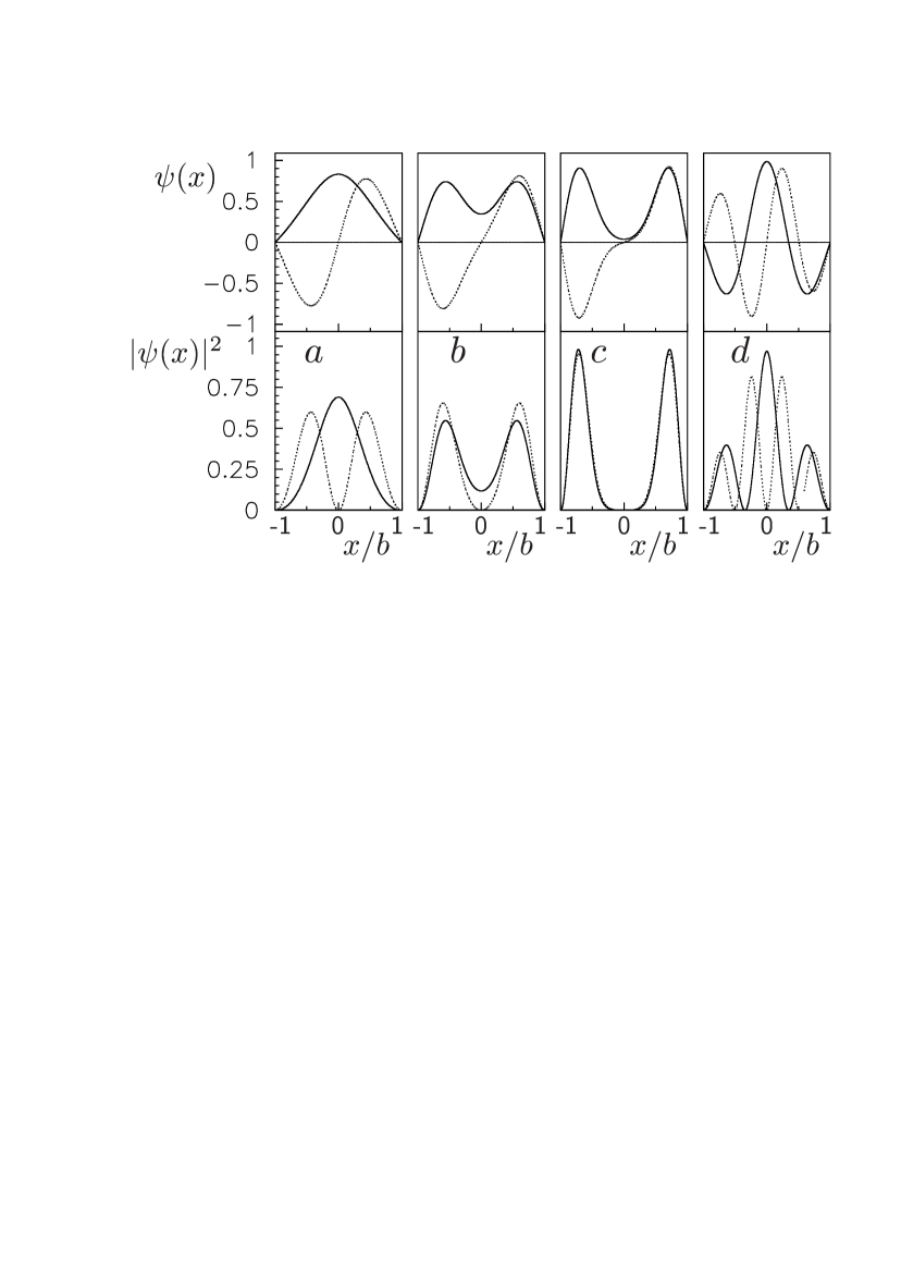
Figure 1: Examples of wavefunctions $\psi_{sJ}(x)$ as a function of $x/b$, for $b=1.73$. Pairs of curves refer to consecutive values of $J$, with even parity (continuous line) or odd parity (dotted line). Part $a:\ J^{\pi}=0^{+},1^{-}$, $b:\ J^{\pi}=10^{+},11^{-}$, $c:\ J^{\pi}=18^{+},19^{-}$ with $s=1$; $d:\ J^{\pi}=0^{+},1^{-}$ with $s=2$. With increasing angular momentum, the difference in $|\psi(x)|^{2}$ between consecutive values of $J$ tends to vanish and, as a consequence, the positive and negative part of the band merge together.

For a given $b$ and for every value of $J$, one obtains a complete set of orthogonal eigenfunctions, with an integrating factor $(1+x^{2})$. These eigenfunctions can be characterized by the quantum number $s=\nu+1$, where $\nu$ is the number of zeroes in the open interval $0<x<b$. A few examples of wavefunctions corresponding to the square–well potential with $b=1.73$ and for different values of $s$ and $J$ are depicted in the Fig. 1.

The dependence of the eigenvalues on the parameter $b$ is illustrated by the Fig. 2, where the ratios $E(J)/E(2)$ are shown for the g.s. band ($s=1$). Other possible choices of the set of independent dynamical variables would have brought to a different equation, but the difference would have concerned the coefficient of the first–derivative term the eq. (34), with very small effect on the results, as long as $b$ is in a range of “reasonable” values. To exemplify the effect of this term, results obtained with the coefficient of the first derivative put to zero are also shown – as dotted lines – in the Figure 2. Differences between the two sets of results turn out to be very limited for small values of $b$ (at least, up to $b\approx 2$).

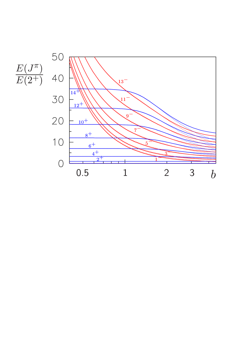
Figure 2: (Color online) Ratio $E(J^{\pi})/E(2^{+})$ as a function of $b$, for states of the ground–state ($s=1$) band with different $J^{\pi}$. Dotted lines show the results obtained with a differential equation corresponding to that of Eq. (34) but without the first–derivative term.

There is at least one case (²²⁶Th) in which our results with the square–well potential are in good agreement with the level scheme, for low-lying states of positive and negative parity, while for ²²⁸Th a better agreement is obtained with the quadratic potential. The possible interpretation of this result as evidence for a phase transition in the octupole degree of freedom is discussed in the next Section.

IV Evidence of phase transition in the octupole degree of freedom

IV.1 The Radium and Thorium isotopic chain

A phase transition in the nuclear shape manifests itself as a relatively sharp change of a proper order parameter – e.g., the ratio $R=E(4^{+})/E(2^{+})$ – as a function of a driving parameter which can be, in our case, the number of neutrons in the isotopes of a given element or the number of protons along an isotone chain. Due to the finite number of degrees of freedom, the transition region has a finite width around the critical point, and extends over several nuclides in the chain. In the case of transitions between spherical shape and axial quadrupole deformation, the X(5) symmetry, valid at the critical point, predicts $E(4^{+})/E(2^{+})=2.91$ and we can use this criterion to locate the critical point of the phase transition.

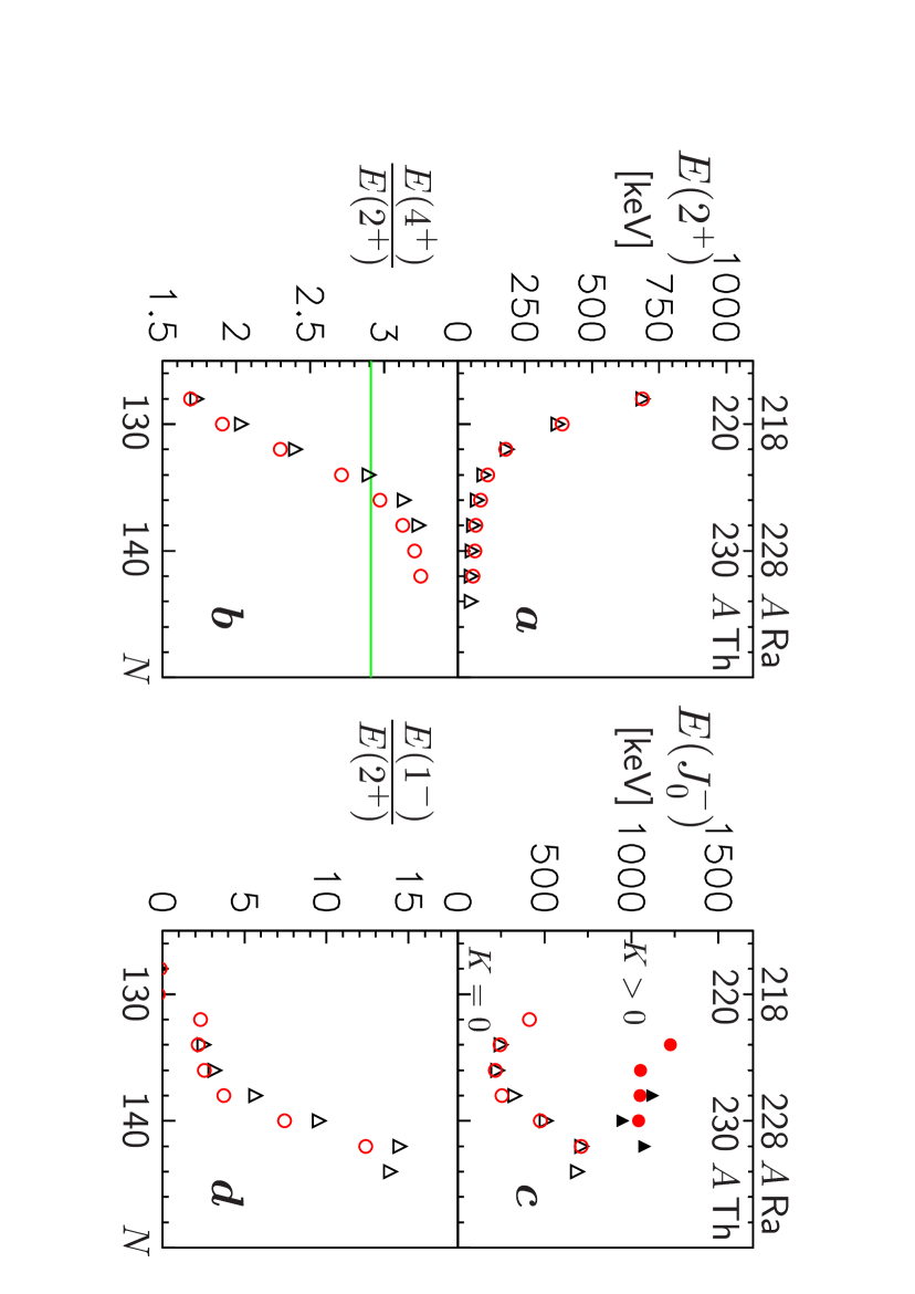
Figure 3: (Color online) Indicators of the quadrupole collectivity (left) and of the octupole collectivity (right), as a function of the neutron number $N$ in the isotopic chain of Ra (circles) and Th (triangles): $a$ - Excitation energy of the first $2^{+}$ level; $b$ - Energy ratio $E(4^{+})/E(2^{+})$; $c$ - Excitation energy of the first level of the $K^{\pi}=0^{-}$ band, $J_{0}^{\pi}=1^{-}$ (open symbols) and of the lowest known level of other negative-parity bands, $J_{0}^{\pi}=2^{-}$ or $1^{-}_{2}$ (full symbols); $d$ - Energy ratio $E(1^{-})/E(2^{+})$. The horizontal line in the part $b$ shows the value (2.91) expected for the X(5) symmetry. Data are from ref.s Cocks et al. (1999); nnd .

The situation is more complex when the quadrupole and the octupole degrees of freedom must be considered at the same time. Fig. 3 shows, as a function of the neutron number of Ra and Th isotopes, a few parameters which can be used as indicators of the quadrupole and octupole collectivity. As for the quadrupole mode, the decrease of $E(2^{+})$ with increasing $N$ (Fig. 3$a$) shows a corresponding increase of collectivity. Moreover, in the Fig. 3$b$ we observe the transition between the vibrational (or not collective) behavior of the lighter isotopes of the chain and a clear rotational behavior ($R\approx 10/3$) above $A=226$, with a critical point which can be located around $A=224$. The ratio $E(1^{-})/E(2^{+})$, depicted in Fig. 3$d$, shows that the relative importance of the octupole collectivity increases with decreasing $N$ and reaches its maximum in the region below $N=138$, where the critical point of the phase transition in the quadrupole mode could be located on the basis of Fig. 3$b$. Heavier isotopes show evidence of octupole vibrations (of different $K$) around a quadrupole-deformed core Guntner et al. (2000); Raduta et al. (1996b). Lighter isotopes ($N<132$) appear not to be deformed in their lower-$J$ states. However, at larger angular momentum a rotational-like band develops, and this band has the alternate-parity pattern typical of a stable octupole deformation Smith et al. (1995).

The model introduced in the first part of this paper, and developed in the section III for the particular case of a permanent quadrupole deformation, assumes that non–axial amplitudes are constrained to very small values by the large restoring forces. This implies that excitation of one of the non–axial degrees of freedom leads to high excitation energy, compared to that of the first $1^{-}$ level of the $K=0$ band. Experimental data of Fig. 3$c$ show that this is actually the case for the light Thorium isotopes, at least up to $A=228$. In fact, the first $1^{-}$ level is not far from the first $2^{+}$ and much lower than levels belonging to negative–parity bands with $K\neq 0$ (as the lowest $2^{-}$ or the second $1^{-}$).

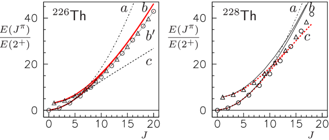
Figure 4: (Color online) Ratios $E(J^{\pi})/E(2^{+})$ as a function of $J$, for positive-parity states (circles) and negative-parity states (triangles) of the ground–state ($s=1$) band of ²²⁶Th and ²²⁸Th, compared with different model calculations: rigid rotor (curve $a$, even parity only), present model at the critical point (curves $b$ and $b^{\prime}$), present model with harmonic potential in $\beta_{3}$ (curve $c$). The curves $b$ and $c$ correspond to a fit on the lowest $1^{-}$ state, the curve $b^{\prime}$, on the $20^{+}$ state. Note that the even-parity parts of the curves $b$ and $b^{\prime}$ are very close to the curve $a$ for $J<6$, while, for each one of the curves $b$, $b^{\prime}$ and $c$, the even- and odd-parity branches tend to merge together at large values of J.

IV.2 Comparison with experimental data for ^226,228Th

Our model assumes a permanent quadrupole deformation. Therefore, it can be useful only for relatively heavy Th isotopes (Fig. 3$a,b$). The quadrupole-deformed region extends above the mass 224 (which could correspond to the critical point of the phase transition, having $E(4^{+})/E(2^{+})\approx 2.91$). Heavier Th isotopes (with $A\geq 230$) show negative-parity bands built on the different states of octupole vibration, from $K=0$ to $K=3$, with band heads much higher than the first $2^{+}$ (Fig. 3$c$). Only for lower $A$, the $1^{-}$ band head of the $K^{\pi}=0^{-}$ band decreases well below the band heads of all other octupole bands, and higher levels of the $K^{\pi}=0^{-}$ band merge with those of positive-parity of the ground-state band (Fig. 4), approaching (but not reaching) the pattern expected for a rigid, reflection asymmetric rotor.

The region of possible validity of our model is therefore restricted to ²²⁶Th and ²²⁸Th.

The ratios $E(J^{\pi})/E(2^{+})$ for the low-lying states of ²²⁶Th and ²²⁸Th are depicted in the Fig. 4, and compared with the predictions of different models. The rigid-rotor model cannot account for the position of the lowest negative-parity levels, and overestimates the excitation energy for all the high-spin states. Instead, a rather good agreement is obtained with the present model, if one assumes, in the case of ²²⁶Th, a square-well potential (as the one hypothesized by Iachello in his X(5) model) and, in the case of ²²⁸Th, a harmonic restoring force. In both cases, the free parameter of the model has been adjusted to reproduce the position of the $1^{-}$ level. As shown in the Fig. 4 (dotted line) a much better agreement with the high-spin levels of ²²⁶Th is obtained with a slightly different value of the parameter ($b=1.87$ instead of 1.73), at the expense of a very limited discrepancy for the $1^{-}$ level.

Therefore, for what concerns the level energies of the ground-state band (including in it also the odd-$J$, negative-parity states), ²²⁶Th seems to present the expected behavior of a nucleus with permanent quadrupole deformation and close to the critical point of the phase transition in the octupole mode.

IV.3 Other possible tests of the critical-point behavior

A considerable amount of experimental information has been reported, in the last few years, on possible candidates Casten and Zamfir (2001); Krucken et al. (2002); Bizzeti and Bizzeti-Sona (2002); Hutter et al. (2003); Clark et al. (2003); Fransen et al. (2004); Bijker et al. (2003, 2004); Tonev et al. (2004) for the dynamical symmetry X(5)(phase transition point in the quadrupole mode). It is now clear that the agreement between experimental and calculated energies for the ground-state band does not automatically imply that a similar agreement exists also for other observables, like the excitation energy of the second $0^{+}$ level (the band head of the $s=2$ band) and the in-band and inter-band transition probabilities. In several transitional nuclei, the excitation energies in the ground-state band are in excellent agreement with the X(5) predictions but the calculated ratios of the $B$(E2) transition probabilities fail to reproduce the experimental ones Clark et al. (2003), unless an ad-hoc second-order term is included in the E2 transition operator Arias (2001); Caprio (2004). It is therefore important to test the predictions of our models also for what concerns such observables.

The low–lying level scheme of ²²⁶Th is shown in the Fig. 5, together with the one resulting from the present model, with the value of $b$ adjusted in order to reproduce the empirical value of the ratio $E(1^{-})/E(2^{+})$.

Figure 5: Experimental level scheme of ²²⁶Th compared with the predictions of the present model at the critical point. The two spectra are normalized on the first $2^{+}$ level, and the model parameter $b$ is adjusted to reproduce the position of the first $1^{-}$.

At the moment, only the first two levels of the $s=2$ band ($0^{+}_{2},\ 2^{+}_{2}$) are known and their excitation energies are somewhat higher than the values predicted at the critical point. We can observe, however, that also in the best X(5) nuclei Casten and Zamfir (2001); Krucken et al. (2002); Tonev et al. (2004) the position of the levels of the $s=2$ band deviates somewhat from the model predictions (although in the opposite direction). In our opinion, a similar qualitative agreement is obtained also in the present case. The negative–parity levels of the $s=2$ band are predicted to lie at higher energies, and could be difficult to observe. Absolute values of the transition strengths are not available for ²²⁶Th, but some relevant information is provided by the branching ratios in the level decays. In the tables 3,4, experimental ratios of the reduced transition strengths for E1 or E2 transitions coming from the same level are compared with the model prediction at the critical point.

Table 3: Experimental and calculated values of the ratios of reduced strengths for E1 transitions coming from the same level of ²²⁶Th.

	Trans. 1		Trans. 2		$B_{i\rightarrow f_{1}}$ (E1)/$B_{i\rightarrow f_{2}}$(E1)
$J^{\pi}_{i}$	$\Rightarrow J^{\pi}_{f_{1}}$		$\Rightarrow J^{\pi}_{f_{2}}$		Theoretical	Experimental
$1^{-}$		$\Rightarrow 0^{+}$		$\Rightarrow 2^{+}$	0.47		0.54	(5)
$3^{-}$		$\Rightarrow 2^{+}$		$\Rightarrow 4^{+}$	0.65		0.99	(25)
$2_{2}^{+}$		$\Rightarrow 1^{-}$		$\Rightarrow 3^{-}$	0.63		0.60	(18)

Table 4: Experimental and calculated values of the ratios of reduced strengths (in W.u.) $R=B(E1)/B(E2)$, for transitions coming from the same level of ²²⁶Th.

	Trans. 1		Trans. 2		$R\ \times\ 10^{5}$
$J^{\pi}_{i}$	$\Rightarrow J^{\pi}_{f1}$		$\Rightarrow J^{\pi}_{f2}$		Theoretical	Experimental
$8^{+}$	E1	$7^{-}$	E2	$6^{+}$	1.3		2.0	(8)
$9^{-}$	E1	$8^{+}$	E2	$7^{-}$	1.3		1.7	(2)
$10^{+}$	E1	$9^{-}$	E2	$8^{+}$	1.6		1.5	(1)
$11^{-}$	E1	$10^{+}$	E2	$9^{-}$	1.6		1.7	(1)
$12^{+}$	E1	$11^{-}$	E2	$10^{+}$	1.8		1.6	(1)
$13^{-}$	E1	$12^{+}$	E2	$11^{-}$	1.8
$14^{+}$	E1	$13^{-}$	E2	$12^{+}$	1.9		1.4	(1)
$15^{-}$	E1	$14^{+}$	E2	$13^{-}$	2.0		1.7	(3)
$16^{+}$	E1	$15^{-}$	E2	$14^{+}$	2.1
$17^{-}$	E1	$16^{+}$	E2	$15^{-}$	2.1		1.5	(3)
$18^{+}$	E1	$17^{-}$	E2	$16^{+}$	2.2
$19^{-}$	E1	$18^{+}$	E2	$17^{-}$	2.3		1.7	(4)

The electric dipole moment would vanish for the collective motion of a fluid with uniform charge density, as the center of charge would coincide with the center of mass. Therefore,the observed E1 transition amplitudes are entirely due to the non uniformity of the nuclear charge distribution Tsvekov et al. (2002). To calculate the value of $B$(E1)$=(i||\mathcal{M}(E1)||f)^{2}/(2J_{i}+1)$, the E1 transition operator has been assumed to have the form Bohr and Mottelson (1957, 1958); Strutinski (1957); Lipas (1963)

$$\mathcal{M}_{\mu}(E1)=C_{1}\beta_{2}\beta_{3}Y_{1,\mu}\ ,$$ (35)

with the constant factor $C_{1}$ depending on the nuclear charge polarizability. The E2 transition operator for the in-band transition and at the limit close to the axial symmetry has been taken in the simple form

$$\mathcal{M}_{\mu}(E2)=C_{2}(\beta_{0})Y_{2,\mu}\ ,$$ (36)

neglecting the (weak) dependence on $\beta_{3}^{2}$. Therefore, the theoretical ratio of the reduced strengths for transitions of different multipolarity (E1 and E2) is determined apart from a constant factor, which must be fixed by comparison with the experimental data. The average of the ratios $B$(E1)/$B$(E2) for the transitions coming from the $10^{+}$ and $11^{-}$ levels has been used for normalization of the theoretical values given in the Table 4.

V Conclusions

A theoretical scheme for the description of quadrupole plus octupole excitations close to the axial symmetry limit has been developed in the Section II and specialized in the Section III to the simpler case of a permanent (and axially symmetric) quadrupole deformation. In principle, the model should be able to describe the wide field of reflection–asymmetric nuclear shapes, close to (but not coincident with!) the axial symmetry limit. Calculations of nuclear shapes in the frame of the HBF-Cranking model Nazarewicz and Olanders (1985) for nuclei of the Radium – Thorium region find a large variety of results, including proper potentials for quadrupole–octupole vibrations around a spherical shape or for octupole vibrations around a deformed, reflection symmetric shape, and also situations with a rather flat minimum of the potential along a line at constant $\beta_{2}$ with $|\beta_{3}|<\beta_{3}^{max}$. The latter case is just what is expected for our “critical point” of the phase transition in the octupole mode. In the Section IV, we have investigated the evolution of the nuclear shape along the isotopic chain of Thorium, and shown that evidence of phase transition exists, not only in the quadrupole mode but also in the octupole mode around a stable quadrupole deformation. The model developed in the Section III results to be able to account for the experimental data of ²²⁶Th (at the critical point of the phase transition in the octupole mode), and also of its neighbor ²²⁸Th (characterized by axial octupole vibrations). More and improved experimental data on E2 and E1 transition strengths would be necessary for a more stringent test of the model predictions.

Further developments of the calculations are in program, to provide detailed predictions for other significant cases: first of all, those of ²²⁴Ra and ²²⁴Th, whose positive–parity levels show an energy sequence very close to Iachello X(5) predictions for the critical point of phase transition between spherical shape and axially symmetric quadrupole deformation.

Appendix A Summary of the general formalism

The general formalism to describe collective states of rotation/vibration in nuclei is discussed e.g. in ref. Bohr (1952). The nuclear surface is described in polar coordinates as

$$r(\theta,\phi)=R_{0}\left[1+\sum_{\lambda}\sum_{\mu=-\lambda,\lambda}\alpha^{(\lambda)}_{\mu}Y^{*}_{\lambda,\mu}(\theta,\phi)\right],$$ (37)

with the condition $\alpha^{(\lambda)}_{-\mu}=(-1)^{\mu}{\alpha^{(\lambda)}_{\mu}}^{*}$.

In the sum, the values of $\lambda$ are now limited to 2,3. A term with $\lambda=1$ should be included in order to maintain fixed the position of the center of mass Eisenberg and Greiner (1987):

$$\alpha^{(1)}_{\mu} = \frac{3}{\sqrt{16\pi}}\ \sum_{\lambda,\lambda^{\prime}}\sqrt{(2\lambda+1)(2\lambda^{\prime}+1)}$$ (40)

$$\cdot\left(\begin{array}[]{ccc}\lambda&\lambda^{\prime}&1\\ 0&0&0\end{array}\right)\ \left[\alpha^{(\lambda)}\otimes\alpha^{(\lambda^{\prime})}\right]^{(1)}_{\mu}\ .$$

This term, however, is inessential for the following discussion, and will be omitted. For not-too-large deformation, in fact, the amplitudes $\alpha^{(1)}_{\mu}$ are much smaller than the others, and their effect results to be negligible for most purposes (with the noticeable exception of the E1 transition amplitudes). At the same level of accuracy, one can also neglect the slight variation of $R_{0}$ necessary to keep the volume exactly constant.

In the Bohr model that we are considering here, the classical expression of the collective kinetic energy is

$$T=\frac{1}{2}B_{2}\sum_{\mu=-2,2}\left|\dot{\alpha}^{(2)}_{\mu}\right|^{2}+\frac{1}{2}B_{3}\sum_{\mu=-3,3}\left|\dot{\alpha}^{(3)}_{\mu}\right|^{2}\ .$$ (41)

In order to simplify the notation in the following, we include the inertia coefficient $B_{\lambda}$ in the definition of the collective variables $a^{(\lambda)}_{\mu}$. In the literature, this symbol is usually reserved to the variables defined in the intrinsic reference frame and, from now on, we will always use this reference frame for the collective variables $a^{(\lambda)}_{\mu}$:

$$\sqrt{B_{\lambda}}\ \alpha^{(\lambda)}_{\mu}=\sum_{\nu}a^{(\lambda)}_{\nu}{D^{(\lambda)}_{\mu\nu}}^{*}(\theta_{i})$$ (42)

where $D^{(\lambda)}$ are the Wigner matrices and $\theta_{i}$ the Euler angles. The axis of the intrinsic reference frame are defined along the principal axis of the inertia tensor.

The expression of the kinetic energy in terms of the time derivatives of the intrinsic deformation variables $a^{(\lambda)}_{\mu}$ and of the angular velocity $\vec{q}$ of the intrinsic frame with respect to an inertial frame is discussed, e.g., in the ref.s Bohr (1952); Eisenberg and Greiner (1987). If only the quadrupole mode is considered, the total kinetic energy can be expressed as the sum of a vibrational term (in the intrinsic frame) and a rotational term. If the octupole mode is also considered, a rotation-vibration coupling term must be added Eisenberg and Greiner (1987); Wexler and Dussel (1999):

$$T=T_{\rm vib}+T_{\rm rot}+T_{\rm coup}$$ (43)

where

$$T_{\rm vib} = \frac{1}{2}\sum_{\lambda,\mu}\left|\dot{a}^{(\lambda)}_{\mu}\right|^{2}$$ (44)

$$T_{\rm rot} = \frac{1}{2}\sum_{\lambda,\nu,\nu^{\prime}}a^{(\lambda)}_{\nu}{a^{(\lambda)}_{\nu^{\prime}}}^{*}\sum_{k,k^{\prime}}q_{k}q_{k^{\prime}}\left(M^{\{\lambda\}}_{k}M^{\{\lambda\}}_{k^{\prime}}\right)_{\nu\nu^{\prime}}$$ (45)

$$\equiv \frac{1}{2}\sum_{k,k^{\prime}}q_{k}q_{k^{\prime}}\mathcal{J}_{kk^{\prime}}\ ,$$

$$T_{\rm coup} = \frac{i}{2}\sum_{\lambda,\nu,\nu^{\prime},k}q_{k}\left[\dot{a}^{(\lambda)}_{\nu}{a^{(\lambda)}_{\nu^{\prime}}}^{*}-a^{(\lambda)}_{\nu}{{\dot{a}}^{(\lambda)*}_{\nu^{\prime}}}\right]\left(M^{\{\lambda\}}_{k}\right)_{\nu,\nu^{\prime}}$$

$$= i \!\sum_{\lambda}\!\sqrt{3(2\lambda\!+\!1)}\left[q^{(1)}\!\otimes\!\left[a^{(\lambda)}\!\otimes\dot{a}^{(\lambda)}\right]^{(1)}\right]^{(0)}_{0}\!.$$ (46)

Here, $q_{k}$ ($k=1,2,3$) are the Cartesian components of the angular velocity $\vec{q}$ along the axes of the intrinsic frame, while the $M^{\{\lambda\}}_{k}$ are $(2\lambda+1)$–dimensional matrices giving the quantum–mechanical representation of the Cartesian components of an angular momentum $M=\lambda$ in the intrinsic frame, subject to commutation rules of the form

$$M^{\{\lambda\}}_{1}M^{\{\lambda\}}_{2}-M^{\{\lambda\}}_{2}M^{\{\lambda\}}_{1}=-iM^{\{\lambda\}}_{3}\ .$$ (47)

We assume, as usually,

$$\left(\right. M^{\{\lambda\}}_{3}\left.\right)_{\nu\nu^{\prime}}=\nu\delta_{\nu,\nu^{\prime}}$$

$$\left(\right. M^{\{\lambda\}}_{1}\left.\right)_{\nu\nu^{\prime}}=\frac{1}{2}\ \left(\sqrt{(\lambda-\nu)\ (\lambda+\nu+1)}\ \delta_{\nu^{\prime},\nu+1}\right.$$

$$+\left.\sqrt{(\lambda+\nu)\ (\lambda-\nu+1)}\ \delta_{\nu^{\prime},\nu-1}\right)$$

$$\left(\right. M^{\{\lambda\}}_{2}\left.\right)_{\nu\nu^{\prime}}=\frac{1}{2}\left(-i\ \sqrt{(\lambda-\nu)\ (\lambda+\nu+1)}\ \delta_{\nu^{\prime},\nu+1}\right.$$

$$+\left.i\ \sqrt{(\lambda+\nu)\ (\lambda-\nu+1)}\ \delta_{\nu^{\prime},\nu-1}\right).$$

Taking into account the properties of the $M^{\{\lambda\}}_{k}$, it is possible to obtain the explicit expression for the diagonal and non diagonal elements of the tensor of inertia Bohr (1952); Wexler and Dussel (1999)

$$\mathcal{J}_{kk^{\prime}}=\frac{1}{2}\sum_{\lambda,\nu,\nu^{\prime}}a^{(\lambda)}_{\nu}{a^{(\lambda)}_{\nu^{\prime}}}^{*}\left(M^{\{\lambda\}}_{k}M^{\{\lambda\}}_{k^{\prime}}+M^{\{\lambda\}}_{k^{\prime}}M^{\{\lambda\}}_{k}\right)_{\nu\nu^{\prime}}\ .$$ (48)

The spin operators $M^{\{\lambda\}}_{k}$ transform as the Cartesian components of a vector $\vec{M}^{\{\lambda\}}$ under rotation in the ordinary space. Taking into account the commutation rule (47), we can define the irreducible tensor components of $\vec{M}^{\{\lambda\}}$ as

$$M^{(1)\{\lambda\}}_{0} = M^{\{\lambda\}}_{3}$$

$$M^{(1)\{\lambda\}}_{\pm 1} = \pm\frac{1}{\sqrt{2}}\left(M^{\{\lambda\}}_{1}\mp i\ M^{\{\lambda\}}_{2}\right)$$ (49)

and express the products of two Cartesian components as the sum of products of two tensor components. To this purpose, we define, for each value of $\lambda$, the irreducible tensor product

$$T^{(J)}_{m} = \left[M^{(1)}\otimes M^{(1)}\right]^{(J)}_{m}$$ (50)

$$\equiv \sum_{\nu,\nu^{\prime}}(1\nu 1\nu^{\prime}|Jm)M^{(1)}_{\nu}\ M^{(1)}_{\nu^{\prime}}$$

(where the common suffix $\{\lambda\}$ has been dropped, for sake of simplicity). We now introduce the reduced matrix elements of the tensor operator $T^{(J)}$,

$$(\lambda||T^{(J)}||\lambda)=(-1)^{J}\sqrt{2J+1}\left\{\!\begin{array}[]{ccc}1&1&J\\ \lambda&\lambda&\lambda\end{array}\!\right\}\lambda(\lambda+1)(2\lambda+1)$$ (51)

to obtain

$$\left(M^{(1)}_{\mu}\ M^{(1)}_{\mu^{\prime}}\right)_{\nu,\nu^{\prime}} = \sum_{Jm}(1\mu 1\mu^{\prime}|Jm)\ \left(T^{(J)}_{m}\right)_{\nu,\nu^{\prime}}$$

$$= \sum_{Jm}(1\mu 1\mu^{\prime}|Jm)(\lambda||T^{(J)}||\lambda)$$

$$\times\frac{(-1)^{\lambda-\nu+m}}{\sqrt{2J+1}}\ (\lambda\nu\lambda-\nu^{\prime}|Jm)\ .$$

We now observe that

$${a^{(\lambda)}_{\nu^{\prime}}}^{*}=(-1)^{\nu^{\prime}}a^{(\lambda)}_{-\nu^{\prime}}$$ (53)

and that

$$\left[a^{(\lambda)}\otimes a^{(\lambda)}\right]^{(J)}_{m}=\sum_{\nu,\nu^{\prime}}a^{(\lambda)}_{\nu}a^{(\lambda)}_{-\nu^{\prime}}\ (\lambda\nu\lambda-\nu^{\prime}|Jm)$$ (54)

to obtain

$$\sum_{\nu,\nu^{\prime}} a^{(\lambda)}_{\nu}{a^{(\lambda)}_{\nu^{\prime}}}^{*}\left(M^{(1)\{\lambda\}}_{\mu}M^{(1)\{\lambda\}}_{\mu^{\prime}}\right)_{\nu\nu^{\prime}}$$ (55)

$$=\sum_{J,m}\frac{(-1)^{\lambda}}{\sqrt{2J+1}}(1\mu 1\mu^{\prime}|Jm)\ (\lambda||T^{(J)}||\lambda)$$

$$\ \times\ \left[a^{(\lambda)}\otimes a^{(\lambda)}\right]^{(J)}_{m}\ .$$

The rank of the tensor product $T^{(J)}$ of the two identical vectors $M^{(1)\{\lambda\}}$ must be even, and therefore the possible values of $J$ are limited to 0 and 2. Now we can substitute, in the eq. (48), the cartesian components of the angular momentum with its tensor components defined in the eq.s (49). The possible values of $m$ (and $J$) contributing to the sum are limited to $m=0$ (and therefore $J=$0 or 2) in the case of $(M_{3})^{2}$, to $m=0$ or 2 ($J=$0 or 2) for $(M_{1})^{2}$, $(M_{2})^{2}$ and $(M_{1}M_{2})$, to $m=1$ ($J=2$) for $(M_{3}M_{1})$ and $(M_{3}M_{2})$. One obtains

$$\mathcal{J}_{1} = \sum_{\lambda}\left\{C_{0}(\lambda)\left[a^{(\lambda)}\otimes a^{(\lambda)}\right]^{(0)}_{0}\right.$$ (56a)

$$+ \frac{1}{\sqrt{6}}C_{2}(\lambda)\left[a^{(\lambda)}\otimes a^{(\lambda)}\right]^{(2)}_{0}$$

$$- \left.C_{2}(\lambda){\rm Re}\left[a^{(\lambda)}\otimes a^{(\lambda)}\right]^{(2)}_{2}\right\}\ ,$$

$$\mathcal{J}_{2} = \sum_{\lambda}\left\{C_{0}(\lambda)\left[a^{(\lambda)}\otimes a^{(\lambda)}\right]^{(0)}_{0}\right.$$ (56b)

$$+ \frac{1}{\sqrt{6}}C_{2}(\lambda)\left[a^{(\lambda)}\otimes a^{(\lambda)}\right]^{(2)}_{0}$$

$$+ \left.C_{2}(\lambda){\rm Re}\left[a^{(\lambda)}\otimes a^{(\lambda)}\right]^{(2)}_{2}\right\}\ ,$$

$$\mathcal{J}_{3} = \sum_{\lambda}\left\{C_{0}(\lambda)\left[a^{(\lambda)}\otimes a^{(\lambda)}\right]^{(0)}_{0}\right.$$ (56c)

$$- \sqrt{\frac{2}{3}}\left.C_{2}(\lambda)\left[a^{(\lambda)}\otimes a^{(\lambda)}\right]^{(2)}_{0}\right\}\ ,$$

$$\mathcal{J}_{12} = \sum_{\lambda}C_{2}(\lambda)\ {\rm Im}\left[a^{(\lambda)}\otimes a^{(\lambda)}\right]^{(2)}_{2}\ ,$$ (56d)

$$\mathcal{J}_{13} = \sum_{\lambda}C_{2}(\lambda)\ {\rm Re}\left[a^{(\lambda)}\otimes a^{(\lambda)}\right]^{(2)}_{1}\ ,$$ (56e)

$$\mathcal{J}_{23} = \sum_{\lambda}C_{2}(\lambda)\ {\rm Im}\left[a^{(\lambda)}\otimes a^{(\lambda)}\right]^{(2)}_{1}.$$ (56f)

where

$$C_{0}(\lambda) = (\!-\!1)^{\lambda}\ \frac{\lambda(\lambda+1)}{3}\sqrt{2\lambda+1}$$

$$C_{2}(\lambda) = (\!-\!1)^{\lambda+1}\ \sqrt{\frac{\lambda(\lambda\!+\!1)(2\lambda\!+\!\!3)(4\lambda^{2}-1)}{30}}$$

and therefore

$$\begin{array}[c]{lp{8mm}l}C_{0}(2)=2\ \sqrt{5}\ ,&&C_{0}(3)=-4\ \sqrt{7}\ ,\\ C_{2}(2)=-\sqrt{21}\ ,&&C_{2}(3)=3\ \sqrt{14}\ .\end{array}$$ (57)

If we chose as the intrinsic reference frame the principal axis of the tensor of inertia, we must put $\mathcal{J}_{12}=\mathcal{J}_{13}=\mathcal{J}_{23}=0$. Using Eq.s (1,2,3) we obtain, up to the first order

$$\mathcal{J}_{12} = -2\ \sqrt{21}\ {\rm Im}\ \left[\bar{a}^{(2)}\otimes\tilde{a}^{(2)}\right]^{(2)}_{2}$$ (58a)

$$+ 6\ \sqrt{14}\ {\rm Im}\ \left[\bar{a}^{(3)}\otimes\tilde{a}^{(3)}\right]^{(2)}_{2}=0,$$

$$\mathcal{J}_{13} + i\mathcal{J}_{23}=-2\ \sqrt{21}\ \left[\bar{a}^{(2)}\otimes\tilde{a}^{(2)}\right]^{(2)}_{1}$$ (58b)

$$+ 6\ \sqrt{14}\ \left[\bar{a}^{(3)}\otimes\tilde{a}^{(3)}\right]^{(2)}_{1}=0\ .$$

Here we make use of the fact that the zero–order terms are automatically set to zero if the $\bar{a}^{(\lambda)}_{\mu}$ are defined according to eq.s (1,2). By inserting these definitions in the above equations, and retaining only the first–order terms, one obtains

$$\left[\bar{a}^{(2)}\otimes\tilde{a}^{(2)}\right]^{(2)}_{1} \approx (2,0,2,1|2,1)\ \beta_{2}\ \tilde{a}^{(2)}_{1}$$

$$= -\frac{1}{\sqrt{14}}\ \beta_{2}\ \tilde{a}^{(2)}_{1}\ ,$$

$${\rm Im}\left[\bar{a}^{(2)}\otimes\tilde{a}^{(2)}\right]^{(2)}_{2} \approx (2,0,2,2|2,2)\ \beta_{2}\ {\rm Im}\ \tilde{a}^{(2)}_{2}$$

$$= \sqrt{\frac{2}{7}}\ \beta_{2}\ {\rm Im}\ \tilde{a}^{(2)}_{2}\ ,$$

$$\left[\bar{a}^{(3)}\otimes\tilde{a}^{(3)}\right]^{(2)}_{1} \approx (3,0,3,1|2,1)\ \beta_{3}\ \tilde{a}^{(3)}_{1}$$

$$= \sqrt{\frac{1}{42}}\ \beta_{3}\ \tilde{a}^{(3)}_{1},$$

$${\rm Im}\left[\bar{a}^{(3)}\otimes\tilde{a}^{(3)}\right]^{(2)}_{2} \approx (3,0,3,2|2,2)\ \beta_{3}\ {\rm Im}\ \tilde{a}^{(3)}_{2}$$

$$= -\sqrt{\frac{5}{21}}\ \beta_{3}\ {\rm Im}\ \tilde{a}^{(3)}_{2}.$$

We obtain, therefore, from eq.s (58)

$$\beta_{2}\tilde{a}^{(2)}_{1} = -\sqrt{2}\ \beta_{3}\tilde{a}^{(3)}_{1},$$

$$\beta_{2}{\rm Im}\ \tilde{a}^{(2)}_{2} = -\sqrt{5}\ \beta_{3}{\rm Im}\ \tilde{a}^{(3)}_{2}.$$ (59)

Appendix B Effect of non diagonal (first-order) terms

The matrix $\mathcal{G}$, as it results from the Table 1, contains zero-order terms only in its principal diagonal (whose last element, however, is small of the second order). Non diagonal terms have been expanded in series up to the first order in the “small” dynamical variables (all of them, apart from $\beta_{2}$ and $\beta_{3}$). We shall call $\xi_{k}$ a generic “small” variable, different from $\beta_{\lambda}$ $(\lambda=2,3)$.

Terms of the last line and column (those related to the third intrinsic component of the angular velocity) are discussed in the Section II.4. Here, we consider a simpler problem: the inversion of a matrix $\mathcal{G}$ which has finite values for all terms in the principal diagonal, and only “small” values for all others. In the zero-order approximation, the inverse matrix $\mathcal{A=G}^{-1}$ is diagonal, with diagonal elements $A_{\mu\mu}=1/G_{\mu\mu}$.

The first–order approximation gives the non–diagonal elements

$$A_{\mu\nu}=A_{\nu\mu}=-\frac{G_{\mu\nu}}{G_{\mu\mu}G_{\nu\nu}}.$$ (60)

We are interested in particular on the effect of non diagonal terms on the coefficients of the derivatives with respect to $\beta_{2}$ or $\beta_{3}$.

Terms involving the derivatives with respect to $\beta_{\lambda}$ and $\xi_{k}$ have the form

$$G^{-\frac{1}{2}}\frac{\partial}{\partial\xi_{k}}\left[G^{\frac{1}{2}}A_{k\lambda}\frac{\partial}{\partial\beta_{\lambda}}\right]+G^{-\frac{1}{2}}\frac{\partial}{\partial\beta_{\lambda}}\left[G^{\frac{1}{2}}A_{\lambda k}\frac{\partial}{\partial\xi_{k}}\right].$$ (61)

The non diagonal matrix elements of the matrix $\mathcal{A}$ are of the first order in the “small” variables. They have therefore the form $f^{(i)}_{\lambda k}(\beta_{2},\beta_{3})\xi_{i}$, where $f^{(i)}_{\lambda k}(\beta_{2},\beta_{3})=\partial\mathcal{A}_{\lambda,k}/\ \partial\xi_{i}$, or – possibly – are the sum of several terms like that.

Substituting this expression in the Eq. (61) one obtains

$$G {}^{-\frac{1}{2}}\frac{\partial}{\partial\xi_{k}}\left[G^{\frac{1}{2}}A_{k\lambda}\frac{\partial}{\partial\beta_{\lambda}}\right]+G^{-\frac{1}{2}}\frac{\partial}{\partial\beta_{\lambda}}\left[G^{\frac{1}{2}}A_{\lambda k}\frac{\partial}{\partial\xi_{k}}\right]$$ (62)

$$= f^{(i)}_{\lambda k}(\beta_{2},\beta_{3})\left[2\xi_{i}\frac{\partial}{\partial\xi_{k}}+\frac{\xi_{i}}{2G}\ \left(\frac{\partial G}{\partial\xi_{k}}\right)+\delta_{ik}\right]\frac{\partial}{\partial\beta_{\lambda}}$$

$$+ \xi_{i}\left[f^{(i)}_{\lambda k}(\beta_{2},\beta_{3})\frac{1}{2G}\ \left(\frac{\partial G}{\partial\beta_{\lambda}}\right)+\left(\frac{\partial f^{(i)}_{\lambda k}}{\partial\beta_{\lambda}}\right)\right]\frac{\partial}{\partial\xi_{k}}\ .$$

The last line of Eq. (62) only contains the partial-derivative operator with respect to the small variable $\xi_{k}$. Compared with the diagonal term involving the corresponding second-derivative operator, it contains a small factor $\xi_{i}$ more, and can be neglected.

In the first line of the expression, all terms are potentially of the same order of magnitude of the leading ones, and in principle could not be neglected. The first of the terms in the square brackets contains the partial derivative with respect to $\xi_{k}$. In the spirit of the adiabatic approach, we try to estimate the expectation value of this term for the ground–state wavefunction in all the variables, with the exception of $\beta_{2}$ and $\beta_{3}$. If we assume that the potential is harmonic for the ensemble of these variables, the ground–state wavefunction can be expected to be close to a multivariate Gaussian function. If, moreover, $\xi_{k}$ and $\xi_{i}$ are uncorrelated, the expectation value of $\xi_{i}\partial/\partial\xi_{k}$ is zero, as $\left<\xi_{i}\right>=0$.

For the case $i=k$, instead, the expectation value is

$$\left<2\xi\frac{\partial}{\partial\xi}\right> \approx 2\ \frac{\int\exp(-\alpha\xi^{2}/2)\xi\frac{\partial}{\partial\xi}\exp(-\alpha\xi^{2}/2){\rm d}\xi}{\int\exp(-\alpha\xi^{2}){\rm d}\xi}$$ (63)

$$= \frac{\int\exp(-\alpha\xi^{2}/2)\left(-2\alpha\xi^{2}\right)\exp(-\alpha\xi^{2}/2){\rm d}\xi}{\int\exp(-\alpha\xi^{2}){\rm d}\xi}$$

$$= -1$$ (64)

and (in this approximation) cancels the third term, $\delta_{ik}$. In conclusion, the coefficient of $\partial/\partial\beta_{\lambda}$ coming from the non–diagonal terms of the matrix ${\mathcal{G}}$ can be approximated with a sum of expressions like

$$\ f^{(i)}_{\lambda k}(\beta_{2},\beta_{3})\ \left<\frac{\xi_{i}}{G}\ \frac{\partial G}{\partial\xi_{k}}\right>$$ (65)

which approximately vanishes for $i\neq k$, and also vanishes for $i=k$ unless both $\mathcal{A}_{\lambda k}$ and $G$ depend explicitly on $\xi_{k}$. Moreover, also in this latter case, it is possible to eliminate non-diagonal elements of the matrix $\mathcal{G}$ of the form $\mathcal{G}_{\lambda k}=\ g_{\lambda k}(\beta_{2},\beta_{3})\ \xi_{k}$, with a slight change in the definition of $\beta_{\lambda}$, without any other effect at the present order of approximation. Namely, it is sufficient to substitute the dynamical variable $\beta_{\lambda}$ with the new variable

$$\beta^{\rm o}_{\lambda}=\beta_{\lambda}+\frac{1}{2}g_{\lambda k}(\beta_{2},\beta_{3})\xi_{k}^{2}$$ (66)

to obtain

$$\dot{\beta}_{\lambda}=\dot{\beta}^{\rm o}_{\lambda}-g_{\lambda k}(\beta_{2},\beta_{3})\xi_{k}\dot{\xi}_{k}+0(\xi_{k}^{2})$$ (67)

and therefore, up to the second order in $\xi_{k}$,

$$\dot{\beta}_{\lambda}^{2} +2g_{\lambda k}(\beta_{2},\beta_{3})\xi_{k}\dot{\beta}_{\lambda}\dot{\xi}_{k}$$ (68)

$$= \left(\dot{\beta}^{\rm o}_{\lambda}-g_{\lambda k}(\beta_{2},\beta_{3})\xi_{k}\dot{\xi}_{k}\right)^{2}+2g_{\lambda k}(\beta_{2},\beta_{3})\xi_{k}\dot{\beta}_{\lambda}\dot{\xi}$$

$$\approx \left(\dot{\beta}^{\rm o}_{\lambda}\right)^{2}.$$

This argument can be easily extended to the case in which the dependence of $\mathcal{A}_{\lambda k}$ on $\xi_{k}$ comes from the dependence on $\xi_{k}$ of one of the terms at the denominator in the eq. (60).

Appendix C Quantization according to the Pauli rule

Table 5: The relevant part of the matrix of inertia, $\mathcal{G}_{1}^{\prime}$, after the substitution of the angular-velocity components $q_{k}$ ($k=1,2,3$) with the time derivative of the Euler angles $\theta_{k}$. Here, $\mathcal{J}_{1}=\mathcal{J}_{2}=3(\beta_{2}^{2}+2\beta_{3}^{2})$, and $\mathcal{J}_{3}=4\ u_{0}^{2}+2v^{2}+8u^{2}+18w^{2}$. The determinant of this $6\times 6$ matrix is now $G_{1}^{\prime}={\rm Det}\ \mathcal{G}_{1}^{\prime}=288\ u_{0}^{2}\ v^{2}u^{2}w^{2}\big{(}\beta_{2}^{2}+2\beta_{3}^{2}\big{)}^{2}\ \sin^{2}\theta_{2}$ .

	$\dot{\varphi}$	$\dot{\chi}$	$\dot{\vartheta}$	$\dot{\theta}_{1}$	$\dot{\theta}_{2}$	$\dot{\theta}_{3}$
$\dot{\varphi}$	$2v^{2}$	0	0	$2v^{2}\cos\theta_{2}$	0	$2v^{2}$
$\dot{\chi}$	0	$2u^{2}$	0	$4u^{2}\cos\theta_{2}$	0	$4u^{2}$
$\dot{\vartheta}$	0	0	$2w^{2}$	$6w^{2}\cos\theta_{2}$	0	$6w^{2}$
$\dot{\theta}_{1}$	$2v^{2}\cos\theta_{2}$	$4u^{2}\cos\theta_{2}$	$6w^{2}\cos\theta_{2}$	$\begin{array}[]{c}(\mathcal{J}_{1}\cos^{2}\theta_{3}+\mathcal{J}_{2}\sin^{2}\theta_{3})\\ \sin^{2}\theta_{3}+\mathcal{J}_{3}\cos^{2}\theta_{2}\end{array}$	$\begin{array}[]{c}(\mathcal{J}_{2}-\mathcal{J}_{1})\sin\theta_{2}\\ \sin\theta_{3}\cos\theta_{3}\end{array}$	$\mathcal{J}_{3}\cos^{2}\theta_{2}$
$\dot{\theta}_{2}$	0	0	0	$\begin{array}[]{c}(\mathcal{J}_{2}-\mathcal{J}_{1})\sin\theta_{2}\\ \sin\theta_{3}\cos\theta_{3}\end{array}$	$\mathcal{J}_{1}\sin^{2}\theta_{3}+\mathcal{J}_{2}\cos^{2}\theta_{3}$	0
$\dot{\theta}_{3}$	$2v^{2}$	$4u^{2}$	$6w^{2}$	$\mathcal{J}_{3}\cos^{2}\theta_{2}$	0	$\mathcal{J}_{3}$

In this Appendix, we discuss some aspects of the quantization of the kinetic energy expression given, e.g., in the eq. (21), by means of the Pauli procedure: namely, if the classical expression of the kinetic energy in terms of the time derivatives of the dynamical variables $\xi_{\mu}$ is

$$T=\frac{1}{2}\sum_{\mu,\nu}\mathcal{G}_{\mu,\nu}\dot{\xi}_{\mu}\dot{\xi}_{\nu}$$ (69)

the corresponding quantum operator has the form

$$\hat{T}=-\frac{\hbar^{2}}{2}G^{-1/2}\sum_{\mu,\nu}\frac{\partial}{\partial\xi_{\mu}}\ G^{1/2}\mathcal{A}_{\mu,\nu}\frac{\partial}{\partial\xi_{\nu}}$$ (70)

where $G={\rm Det}\ \mathcal{G}$ and $\mathcal{A}=\mathcal{G}^{-1}$. The choice of the “best set” of dynamical variables is, in part, related to the expression of the potential-energy term, and it is not obvious that it will eventually coincide with the one discussed in the section II.5. However, it can be useful to explore the properties of the kinetic-energy operator in the particular model in which the matrix of coefficients ${\mathcal{G}}$ is exactly that of the Table 2, with the non-diagonal terms confined in one single line (and column) of the lower $6\times 6$ sub-matrix.

Table 6: The matrix $i(\mathcal{G}_{1}^{\prime})^{-1}\widetilde{W}\sin\theta_{2}$ (see text).

	$\hat{p}_{\varphi}$	$\hat{p}_{\chi}$	$\hat{p}_{\vartheta}$	$\hat{L}_{1}$	$\hat{L}_{2}$	$\hat{L}_{3}$
$\frac{\partial}{\partial\varphi}$	$\frac{\sin\theta_{2}}{2v^{2}}+\frac{\sin\theta_{2}}{4u_{0}^{2}}$	$\frac{2\sin\theta_{2}}{4u_{0}^{2}}$	$\frac{3\sin\theta_{2}}{4u_{0}^{2}}$	0	0	$-\frac{\sin\theta_{2}}{4u_{0}^{2}}$
$\frac{\partial}{\partial\chi}$	$\frac{2\sin\theta_{2}}{4u_{0}^{2}}$	$\frac{\sin\theta_{2}}{2u^{2}}+\frac{4\sin\theta_{2}}{4u_{0}^{2}}$	$\frac{6\sin\theta_{2}}{4u_{0}^{2}}$	0	0	$-\frac{2\sin\theta_{2}}{4u_{0}^{2}}$
$\frac{\partial}{\partial\vartheta}$	$\frac{3\sin\theta_{2}}{4u_{0}^{2}}$	$\frac{6\sin\theta_{2}}{4u_{0}^{2}}$	$\frac{\sin\theta_{2}}{2w^{2}}+\frac{9\sin\theta_{2}}{4u_{0}^{2}}$	0	0	$-\frac{3\sin\theta_{2}}{4u_{0}^{2}}$
$\frac{\partial}{\partial\theta_{1}}$	0	0	0	$-\frac{\cos\theta_{3}}{\mathcal{J}_{1}}$	$\frac{\sin\theta_{3}}{\mathcal{J}_{2}}$	0
$\frac{\partial}{\partial\theta_{2}}$	0	0	0	$\frac{\sin\theta_{2}\sin\theta_{3}}{\mathcal{J}_{1}}$	$\frac{\sin\theta_{2}\cos\theta_{3}}{\mathcal{J}_{2}}$	0
$\frac{\partial}{\partial\theta_{3}}$	$-\frac{\sin\theta_{2}}{4u_{0}^{2}}$	$-\frac{2\sin\theta_{2}}{4u_{0}^{2}}$	$-\frac{3\sin\theta_{2}}{4u_{0}^{2}}$	$\frac{\cos\theta_{2}\cos\theta_{3}}{\mathcal{J}_{1}}$	$-\frac{\cos\theta_{2}\sin\theta_{3}}{\mathcal{J}_{2}}$	$\frac{\sin\theta_{2}}{4u_{0}^{2}}$

From now on, we limit our discussion to the lowest $6\times 6$ sub-matrix $\mathcal{G}_{1}$ of the matrix $\mathcal{G}$ (and of the matrices derived from $\mathcal{G}$, Tables 6 ,7) as the six corresponding variables – $\varphi,\ \chi,\ \vartheta,\ \theta_{1},\ \theta_{2},\ \theta_{3}$ – are effectively decoupled from the others.

The formal procedure is discussed, e.g., in the Ch.s 5 and 6 of the ref. Eisenberg and Greiner (1987). The first pass is the substitution of the intrinsic components $q_{1},\ q_{2},\ q_{3}$ of the angular velocity with the time derivatives of the three Euler angles $\theta_{1},\ \theta_{2},\ \theta_{3}$:

$$q_{k}=\sum_{i}V_{ki}\dot{\theta}_{i}$$ (71)

with

$$V=\left|\begin{array}[]{ccc}-\cos\theta_{3}\sin\theta_{2}&\sin\theta_{3}&0\\ \phantom{-}\sin\theta_{3}\sin\theta_{2}&\cos\theta_{3}&0\\ \cos\theta_{2}&0&1\\ \end{array}\right|\ .$$ (72)

As a consequence of this substitution, the $6\times 6$ matrix $\mathcal{G}_{1}$ transforms according to the relation

$$\mathcal{G}_{1}^{\prime}=\widetilde{W}\ \ \mathcal{G}_{1}\ W,\hskip 56.9055ptW=\left|\begin{array}[]{cc}\{1\}&\{0\}\\ \{0\}&V\end{array}\right|$$ (73)

(where $\widetilde{W}$ is the transpose of the matrix $W$ and $\{1\}$, $\{0\}$ are the $3\times 3$ unit matrix and null matrix) and takes the form shown in the Table 5.

Table 7: The lowest $6\times 6$ sub-matrix of the inverse of the matrix $\mathcal{G}$ given in the Table 2. The upper part is diagonal in the present approximation.

	$\hat{p}_{\varphi}$	$\hat{p}_{\chi}$	$\hat{p}_{\vartheta}$	$\hat{L}_{1}$	$\hat{L}_{2}$	$\hat{L}_{3}$
$\hat{p}_{\varphi}$	$\frac{1}{2v^{2}}+\frac{1}{4u_{0}^{2}}$	$\frac{2}{4u_{0}^{2}}$	$\frac{3}{4u_{0}^{2}}$	0	0	$-\frac{1}{4u_{0}^{2}}$
$\hat{p}_{\chi}$	$\frac{2}{4u_{0}^{2}}$	$\frac{1}{2u^{2}}+\frac{4}{4u_{0}^{2}}$	$\frac{6}{4u_{0}^{2}}$	0	0	$-\frac{2}{4u_{0}^{2}}$
$\hat{p}_{\vartheta}$	$\frac{3}{4u_{0}^{2}}$	$\frac{6}{4u_{0}^{2}}$	$\frac{1}{2w^{2}}+\frac{9}{4u_{0}^{2}}$	0	0	$-\frac{3}{4u_{0}^{2}}$
$\hat{L}_{1}$	0	0	0	$\frac{1}{\mathcal{J}_{1}}$	0	0
$\hat{L}_{2}$	0	0	0	0	$\frac{1}{\mathcal{J}_{2}}$	0
$\hat{L}_{3}$	$-\frac{1}{4u_{0}^{2}}$	$-\frac{2}{4u_{0}^{2}}$	$-\frac{3}{4u_{0}^{2}}$	0	0	$\frac{1}{4u_{0}^{2}}$

The next step is the inversion of the matrix $\mathcal{G}_{1}^{\prime}$. In doing this, the explicit form (20) of $\mathcal{J}_{3}$ has been introduced and second-order terms in the small amplitudes have been neglected. At this point, it is necessary to introduce the intrinsic components of the angular momentum operator ($L_{1},\ L_{2},\ L_{3}$) in the place of the derivatives with respect to the Euler angles. The expression of $L_{k}$ in terms of $\partial/\partial\theta_{k}$ and vice-versa are given, e.g. in the Ch. 5 of ref Eisenberg and Greiner (1987). One gets

$$-i\frac{\partial}{\partial\theta_{k}}=\sum V_{ik}\hat{L}_{i}$$ (74)

with the matrix $V$ given by the eq. (72). It is also convenient to define the quantum operators

$$\hat{p}_{\varphi} = -i\partial\ /\ \partial\varphi$$

$$\hat{p}_{\chi} = -i\partial\ /\ \partial\chi$$

$$\hat{p}_{\vartheta} = -i\partial\ /\ \partial\vartheta$$ (75)

to obtain

$$-i \left\{\frac{\partial}{\partial\varphi},\ \frac{\partial}{\partial\chi},\ \frac{\partial}{\partial\vartheta},\ \frac{\partial}{\partial\theta_{1}},\ \frac{\partial}{\partial\theta_{2}},\ \frac{\partial}{\partial\theta_{3}}\right\}$$ (76)

$$=\ \widetilde{W}\ \left\{\hat{p}_{\varphi},\ \hat{p}_{\chi},\ \hat{p}_{\vartheta},\ \hat{L}_{1},\ \hat{L}_{2},\ \hat{L}_{3}\right\}.$$

The introduction of a set of conjugate momenta $\hat{p}_{k}$ such that

$$-i\frac{\partial}{\partial\xi_{k}}=\sum_{i}W_{ik}\hat{p}_{i}$$ (77)

in the eq. (70) gives

$$\hat{T} = \frac{\hbar^{2}}{2}\left[\sum_{\mu,\nu}(W\mathcal{A}\widetilde{W})_{\mu,\nu}\ \hat{p}_{\mu}\hat{p}_{\nu}\right.$$ (78)

$$\left.+i\ G^{-1/2}\sum_{\mu,\nu}\frac{\partial\ G^{1/2}(\mathcal{A}\widetilde{W})_{\mu,\nu}}{\partial\xi_{\mu}}\ \hat{p}_{\nu}\right].$$

In our case, $\mathcal{A}=(\mathcal{G}_{1}^{\prime})^{-1}$, $\mathcal{G}_{1}^{\prime}=\widetilde{W}\mathcal{G}_{1}W$, so that

$$W\mathcal{A}\widetilde{W}=W\left(W^{-1}\mathcal{G}_{1}^{-1}\widetilde{W}^{-1}\right)\widetilde{W}=\mathcal{G}_{1}^{-1}$$ (79)

and the first term of the eq. (78) takes the form given in the Table 7. The second term of the eq. (78) vanishes. In fact, only the derivatives with respect to $\theta_{2}$ or $\theta_{3}$ could give a contribution to the sum, as the other variables do not appear in the elements of the sub-matrix. Moreover, the determinant $G_{1}$ is simply proportional to $\sin^{2}\theta_{2}$ (with the proportionality factor depending on dynamical variables which are outside the present sub-space), and the term $G^{1/2}$ in the equation (78) can be replaced by $\sin\theta_{2}$. The matrix $i(\mathcal{G}_{1}^{\prime})^{-1}\widetilde{W}\sin\theta_{2}$ is given in the Table 6. The sum of the derivatives of each element of the 5th row, with respect to $\theta_{2}$, plus the corresponding one of the 6th row, with respect to $\theta_{3}$, would give the coefficient of the corresponding momentum operator, but it is easy to verify they cancel each other.

Table 8: Invariants up to the fourth order built with the tensors $a^{(2)}$ and $a^{(3)}$, in the limit close to axial symmetry. Here $T^{(L)}_{KK}\equiv\big{[}a^{K}\otimes a^{K}\big{]}^{(L)}$, and we use the definitions $v^{2}=\eta^{2}+\zeta^{2}$ , $w^{2}=X^{2}+Y^{2}$. “Small” (non-axial) terms are approximated up to the second order.

$A_{1}\equiv$	$\big{(}a^{(2)}\cdot a^{(2)}\big{)}=$	$\beta_{2}^{2}$			$+\frac{10\beta_{3}^{2}}{\beta_{2}^{2}+5\beta_{3}^{2}}\xi^{2}$	$+\frac{4\beta_{3}^{2}}{\beta_{2}^{2}+2\beta_{3}^{2}}v^{2}$
$A_{2}\equiv$	$-\big{(}a^{(3)}\cdot a^{(3)}\big{)}=$	$\beta_{3}^{2}$		$+10w^{2}$	$+\frac{2\beta_{2}^{2}}{\beta_{2}^{2}+5\beta_{3}^{2}}\xi^{2}$	$+\frac{2\beta_{2}^{2}}{\beta_{2}^{2}+2\beta_{3}^{2}}v^{2}$
$B_{1}\equiv$	$-\frac{\sqrt{14}}{4}\ \big{(}a^{(2)}\cdot T^{(2)}_{22}\big{)}=$	$\beta_{2}^{3}$	$-\frac{9}{2}\beta_{2}^{3}\gamma_{2}^{2}$		$-\frac{30\beta_{2}\beta_{3}^{2}}{\beta_{2}^{2}+5\beta_{3}^{2}}\xi^{2}$	$+\frac{6\beta_{2}\beta_{3}^{2}}{\beta_{2}^{2}+2\beta_{3}^{2}}v^{2}$
$B_{2}\equiv$	$\frac{\sqrt{21}}{2}\ \big{(}a^{(2)}\cdot T^{(2)}_{33}\big{)}=$	$\beta_{2}\beta_{3}^{2}$	$-\beta_{2}\beta_{3}^{2}\ \big{(}\frac{1}{2}\gamma_{2}^{2}+\sqrt{5}\gamma_{2}\gamma_{3}+\gamma_{3}^{2}\big{)}$	$-\frac{25}{2}\beta_{2}w^{2}$	$+\frac{10\beta_{2}\beta_{3}^{2}}{\beta_{2}^{2}+5\beta_{3}^{2}}\xi^{2}$	$\frac{3\beta_{2}^{3}-4\beta_{2}\beta_{3}^{2}}{2(\beta_{2}^{2}+2\beta_{3}^{2})}v^{2}$
$C_{1}\equiv$	$\frac{7}{2}\ \big{(}T^{(2)}_{22}\cdot T^{(2)}_{22}\big{)}=$	$\beta_{2}^{4}$			$+\frac{20\beta_{2}^{2}\beta_{3}^{2}}{\beta_{2}^{2}+5\beta_{3}^{2}}\xi^{2}$	$+\frac{8\beta_{2}^{2}\beta_{3}^{2}}{\beta_{2}^{2}+2\beta_{3}^{2}}v^{2}$
$C_{2}\equiv$	$\frac{35}{18}\ \big{(}T^{(4)}_{22}\cdot T^{(4)}_{22}\big{)}=$	$\beta_{2}^{4}$			$+\frac{20\beta_{2}^{2}\beta_{3}^{2}}{\beta_{2}^{2}+5\beta_{3}^{2}}\xi^{2}$	$+\frac{8\beta_{2}^{2}\beta_{3}^{2}}{\beta_{2}^{2}+2\beta_{3}^{2}}v^{2}$
$C_{3}\equiv$	$\frac{21}{4}\ \big{(}T^{(2)}_{33}\cdot T^{(2)}_{33}\big{)}=$	$\beta_{3}^{4}$	$+3\beta_{3}^{4}\gamma_{3}^{2}$	$-25\beta_{3}^{2}w^{2}$	$+\frac{10\beta_{2}^{2}\beta_{3}^{2}}{\beta_{2}^{2}+5\beta_{3}^{2}}\xi^{2}$	$+\frac{4\beta_{2}^{2}\beta_{3}^{2}}{\beta_{2}^{2}+2\beta_{3}^{2}}v^{2}$
$C_{4}\equiv$	$\frac{77}{18}\ \big{(}T^{(4)}_{33}\cdot T^{(4)}_{33}\big{)}=$	$\beta_{3}^{4}$	$-4\beta_{3}^{4}\gamma_{3}^{2}$	$+80\beta_{3}^{2}w^{2}$	$-\frac{4\beta_{2}^{2}\beta_{3}^{2}}{\beta_{2}^{2}+5\beta_{3}^{2}}\xi^{2}$	$+\frac{4\beta_{2}^{2}\beta_{3}^{2}}{\beta_{2}^{2}+2\beta_{3}^{2}}v^{2}$
$C_{5}\equiv$	$\frac{231}{100}\ \big{(}T_{33}^{(6)}\cdot T^{(6)}_{33}\big{)}=$	$\beta_{3}^{4}$	$+\frac{21}{25}\beta_{3}^{4}\gamma_{3}^{2}$	$+\frac{37}{5}\beta_{3}^{2}w^{2}$	$+\frac{142\beta_{2}^{2}\beta_{3}^{2}}{25(\beta_{2}^{2}+5\beta_{3}^{2})}\xi^{2}$	$+\frac{4\beta_{2}^{2}\beta_{3}^{2}}{\beta_{2}^{2}+2\beta_{3}^{2}}v^{2}$
$C_{6}\equiv$	$-\frac{7\sqrt{6}}{4}\big{(}T^{(2)}_{22}\cdot T^{(2)}_{33}\big{)}=$	$\beta_{2}^{2}\beta_{3}^{2}$	$-\beta_{2}^{2}\beta_{3}^{2}\big{(}2\gamma_{2}^{2}-2\sqrt{5}\gamma_{2}\gamma_{3}+\gamma_{3}^{2}\big{)}$	$-\frac{25}{2}\beta_{2}^{2}w^{2}$	$-\frac{20\beta_{2}^{2}\beta_{3}^{2}+10\beta_{3}^{4}}{\beta_{2}^{2}+5\beta_{3}^{2}}\xi^{2}$	$+\frac{3\beta_{2}^{4}-4\beta_{2}^{2}\beta_{3}^{2}+4\beta_{3}^{4}}{2(\beta_{2}^{2}+2\beta_{3}^{2})}v^{2}$
$C_{7}\equiv$	$-\frac{7\sqrt{55}}{18}\big{(}T^{(4)}_{22}\cdot T^{(4)}_{33}\big{)}=$	$\beta_{2}^{2}\beta_{3}^{2}$	$-\frac{1}{6}\beta_{2}^{2}\beta_{3}^{2}\big{(}5\gamma_{2}^{2}+2\sqrt{5}\gamma_{2}\gamma_{3}+13\gamma_{3}^{2}\big{)}$	$+5\beta_{2}^{2}w^{2}$	$+\frac{-7\beta_{2}^{4}+10\beta_{2}^{2}\beta_{3}^{2}+5\beta_{3}^{4}}{3(\beta_{2}^{2}+5\beta_{3}^{2})}\xi^{2}$	$+\frac{\beta_{2}^{4}-20\beta_{2}^{2}\beta_{3}^{2}-8\beta_{3}^{4}}{3(\beta_{2}^{2}+2\beta_{3}^{2})}v^{2}$

Appendix D The possible forms of the potential term

The form of the approximate potential–energy expression depends on the details of the underlying microscopic structure that the model should try to simulate. There are, however, some general rules to which the expression of the potential energy must conform: it must be invariant under space rotation, time reversal, and parity.

Irreducible tensors of different rank have been constructed with each of the basic tensors $a^{(2)}$ and $a^{(3)}$, and scalar products of tensors of equal rank have been considered. In order to be invariant under time reversal, each term must contain an even number of octupole amplitudes $a^{(3)}_{\mu}$. Moreover, due to symmetry, only tensors $T^{(K)}_{\lambda\lambda}=[a^{(\lambda)}\otimes a^{(\lambda)}]^{(K)}$ of even rank $K$ can be obtained with the coupling of two identical tensors $a^{(\lambda)}$. There are therefore two independent invariants of order 2, $\big{(}a^{(2)}\cdot a^{(2)}\big{)}$ and $\big{(}a^{(3)}\cdot a^{(3)}\big{)}$, two of order 3, $\big{(}a^{(2)}\cdot T^{(2)}_{22}\big{)}$ and $\big{(}a^{(2)}\cdot T^{(2)}_{33}\big{)}$, and seven of order 4, namely $\big{(}T^{(K)}_{22}\cdot T^{(K)}_{22}\big{)}$ ($K=2,4$), $\big{(}T^{(K)}_{33}\cdot T^{(K)}_{33}\big{)}$ ($K=2,4,6$), and $\big{(}T^{(K)}_{22}\cdot T^{(K)}_{33}\big{)}$ ($K=2,4$). Additional fourth-order invariants of the form $\big{(}[a^{(2)}\otimes a^{(3)}]^{(K)}\cdot[a^{(2)}\otimes a^{(3)}]^{(K)}\big{)}$ ($K=1-5$), are not independent from the above ones, and can be expressed as linear combination of them with the standard rules of angular momentum recoupling.

Invariant expressions up to the fourth order in the amplitudes $a^{(\lambda)}_{\mu}$ ($\lambda=2,3$) are shown in the Table 8, in terms of the dynamical variables $\beta_{2}$, $\gamma_{2}$, $\beta_{3}$, $\gamma_{3}$, $w^{2}=(X^{2}+Y^{2})$, $\xi$, and $v^{2}=(\eta^{2}+\zeta^{2})$. Expressions corresponding to different choices of the dynamical variables can be easily obtained.

Here, only the terms up to the second order in the series expansion of the “small” (non-axial) amplitudes are given. In this approximation, the fourth-order invariants built with the quadrupole amplitudes ($C_{1},\ C_{2}$) result to be proportional to each other and to the square of the corresponding second-order invariant ($A_{1}^{2}$). Moreover, as it is clear from the Table 8, the three fourth-order invariants built with the octupole amplitudes ($C_{3},\ C_{4},\ C_{5}$) and the square of the corresponding second-order invariant ($A_{2}^{2}$) are not linearly independent of one another, and provide only two independent relations.

One can finally observe that the variables $X,\ Y,\ \eta$ and $\zeta$ always appear only in the combinations $(X^{2}+Y^{2})$, $(\eta^{2}+\zeta^{2})$. As long as the expression of the potential energy does only depend on the invariants up to the fourth order, the angles $\vartheta$ and $\varphi$ defined in the Eq. (17) are not subject to a restoring force. The situation is more complicated for the three variables related to the $\mu=\pm 2$ components of $a^{\lambda}_{\mu}$. Also in this case, however, it is possible to construct combinations of invariants that contain only linear combinations of the squares of the variables $\xi$, $\gamma=\sqrt{5}\gamma_{2}-\gamma_{3}$, and $\gamma_{0}=\beta_{2}^{2}\gamma_{2}+\sqrt{5}\beta_{3}^{2}\gamma_{3}$. Moreover, in this case, the first two of them do appear in the combination $\beta_{2}\beta_{3}\gamma^{2}+2\big{(}\beta_{2}^{2}+5\beta_{3}^{2}\big{)}\xi^{2}$. It is therefore possible to imaging a situation in which the potential energy is independent also of the angle $\chi$ (although this is is not a direct consequence of the model, as it is the case for the angles $\vartheta$ and $\varphi$).

References

• Iachello (2000a) F. Iachello, Phys. Rev. Lett. 85, 3580 (2000a).
• Iachello (2000b) F. Iachello, Phys. Rev. Lett. 87, 052502 (2000b).
• Iachello (2001) F. Iachello, Phys. Rev. Lett. 91, 132502 (2001).
• Casten and Zamfir (2001) R. F. Casten and N. V. Zamfir, Phys. Rev. Lett. 87, 052503 (2001).
• Krucken et al. (2002) R. Krucken, B. Albanna, C. Bialik, R. F. Casten, J. R. Cooper, A. Dewald, N. V. Zamfir, C. J. Barton, C. W. Beausang, M. A. Caprio, et al., Phys. Rev. Lett. 88, 232501 (2002).
• Bizzeti (2003) P. G. Bizzeti, in Symmetries in Physics, edited by A. Vitturi and R. Casten (World Scientific, Singapore, 2003).
• Bizzeti and Bizzeti-Sona (2002) P. G. Bizzeti and A. M. Bizzeti-Sona, Phys. Rev. C 66, 031301 (2002).
• Hutter et al. (2003) C. Hutter et al., Phys. Rev. C 67, 054315 (2003).
• Clark et al. (2003) R. M. Clark et al., Phys. Rev. C 68, 037301 (2003).
• Fransen et al. (2004) C. Fransen, N. Pietralla, A. Linnemann, V.Werner, and R.Bijker, Phys. Rev. C 69, 014313 (2004).
• Tonev et al. (2004) D. Tonev, A. Dewald, T. Klug, P. Petkov, J. Jolie, A. Fitzler, O. Moller, S. Heinze, P. von Brentano, and R. F. Casten, Phys. Rev. C 69, 034334 (2004).
• Bijker et al. (2003) R. Bijker, R. F. Casten, N. V. Zamfir, and E. A. McCutchan, Phys. Rev. C 68, 064304 (2003).
• Bijker et al. (2004) R. Bijker, R. F. Casten, N. V. Zamfir, and E. A. McCutchan, Phys. Rev. C 69, 059901(E) (2004).
• Caprio (2004) M. A. Caprio, Phys. Rev.C 69, 044307 (2004).
• Bonatsos et al. (2004) D. Bonatsos, D. Lenis, N. Minkov, D. Petrellis, P. P. Raychev, and P. A. Terziev, Phys. Rev. C 70, 024305 (2004).
• Pietralla and Gorbachenko (2004) N. Pietralla and O. Gorbachenko, Phys. Rev. C 70, 011304 (2004).
• Bizzeti and Bizzeti-Sona (2004) P. G. Bizzeti and A. M. Bizzeti-Sona, Europ. J. Phys. A 20, 179 (2004).
• Bohr (1952) D. A. Bohr, Dan. Mat. Fys. Medd. 26 (1952), (n.14).
• Engel and Iachello (1985) J. Engel and F. Iachello, Phys. Rev. Lett. 54, 1126 (1985).
• Alonso et al. (1995) C. E. Alonso, J. M. Arias, A. Frank, H. M. Sofia, S. M. Lenzi, and A. Vitturi, Nucl. Phys. A 586, 100 (1995).
• Raduta and Ionescu (2003) A. A. Raduta and D. Ionescu, Phys. Rev. C 67, 044312 (2003), (and references therein).
• Raduta et al. (1996a) A. A. Raduta, D. Ionescu, I. Ursu, and A. Faessler, Nucl. Phys. A 720 (1996a).
• Zamfir and Kusnezov (2001) N. V. Zamfir and D. Kusnezov, Phys. Rev. C 63, 054306 (2001).
• Zamfir and Kusnezov (2003) N. V. Zamfir and D. Kusnezov, Phys. Rev. C 67, 014305 (2003).
• Shneidman et al. (2002) T. M. Shneidman, G. G. Adamian, N. V. Antonenko, R. Jolos, and W. Scheid, Phys. Letters B 526, 322 (2002).
• Rohozinski (1988) S. Rohozinski, Rep. Progr. Phys. 51, 541 (1988).
• Butler and Nazarewicz (1996) P. A. Butler and W. Nazarewicz, Rev. Mod. Phys. 68, 349 (1996), (and references therein).
• Lipas and Davidson (1961) P. O. Lipas and J. P. Davidson, Nucl. Phys. 26, 80 (1961).
• Denisov and Dzyublik (1995) V. Y. Denisov and A. Dzyublik, Nucl. Phys. A 589, 17 (1995).
• Jolos and von Brentano (1999) R. V. Jolos and P. von Brentano, Phys. Rev. C 60, 064317 (1999).
• Minkov et al. (2000) N. Minkov, S. B. Drenska, P. P. Raychev, R. P. Roussev, and D. Bonatsos, Phys. Rev. C 63, 044305 (2000).
• Minkov et al. (2004) N. Minkov, S. Drenska, P. Yotov, and W. Scheid, in Proceedings of the 23rd International Workshop on Nuclear Theory (Rila, Bulgaria 2004), edited by S. Dimitrova (Heron Press, Sofia, 2004).
• Donner and Greiner (1966) W. Donner and W. Greiner, Z. Phys. 197, 440 (1966).
• Eisenberg and Greiner (1987) J. M. Eisenberg and W. Greiner, Nuclear Theory, vol. I (North Holland, Amsterdam, 1987), 3rd ed.
• Wexler and Dussel (1999) C. Wexler and G. G. Dussel, Phys. Rev. C 60, 014305 (1999).
• Wilets and Jean (1956) L. Wilets and M. Jean, Phys. Rev. 102, 788 (1956).
• Pauli (1933) W. Pauli, in Handbook der Physik, edited by A. Smekal (Springer, Berlin, 1933), vol. XXIV/I.
• Abramowitz and Stegun (1970) M. Abramowitz and I. A. Stegun, Handbook of mathematical functions (New York, 1970), section 21.6.
• (39) ENSDF data base, http//:www.nndc.bnl.gov.
• Cocks et al. (1999) J. C. F. Cocks et al., Nucl. Phys. A 645, 61 (1999).
• Guntner et al. (2000) C. Guntner, R. Krucken, C. J. Barton, C. W. Beausang, R. F. Casten, G. Cata-Danil, J. R. Cooper, J. Groeger, J. Novak, and N. V. Zamfir, Phys. Rev. C 61, 064602 (2000).
• Raduta et al. (1996b) A. A. Raduta, N. Lo Judice, and I. Ursu, Nucl. Phys. A 608 (1996b).
• Smith et al. (1995) J. F. Smith et al., Phys. Rev. Lett. 75, 1050 (1995).
• Arias (2001) J. M. Arias, Phys. Rev. C 63, 034308 (2001).
• Tsvekov et al. (2002) A. Tsvekov, J. Kvasil, and R. Nazmitdinov, J. Phys. G: Nucl. Part. Phys. 28, 2187 (2002).
• Bohr and Mottelson (1957) D. A. Bohr and B. R. Mottelson, Nucl. Phys. 4 (1957).
• Bohr and Mottelson (1958) D. A. Bohr and B. R. Mottelson, Nucl. Phys. 9 (1958).
• Strutinski (1957) V. Strutinski, J. Nucl. Energy 4 (1957).
• Lipas (1963) P. O. Lipas, Nucl. Phys. 40 (1963).
• Nazarewicz and Olanders (1985) W. Nazarewicz and P. Olanders, Nucl. Phys. A 441, 420 (1985).