Abstract

A review is given of attempts to bridge the gap between everyday particle and nuclear physics — involving many quarks — and the basic underlying theory of QCD that can only be evaluated exactly for few quark systems. Even the latter requires the original theory of QCD to be discretised to give Lattice QCD — but this modification can still yield exact results for the original theory. These LQCD results can then be considered on a similar footing to experimental data — namely as cornerstones that must be fitted by phenomenological models. In this way, the hope is that “QCD inspired” models can become more and more “QCD based” models, by fixing — in the few-quark case where LQCD can be carried out — the form of these models in such a way that they can be extended to multi-quark systems.

Chapter 0 Bridges from Lattice QCD to Nuclear Physics

A.M. Green

1 Introduction

Even though for over 30 years QCD has been thought to be the theory of strong interactions, it has had a rather limited impact on most other branches of physics — except for few-quark hadron physics. Of course, the reason is well known — to write down the Lagrangian that describes exactly the quark and gluon interactions is easy, but actually performing calculations directly with this Lagrangian has turned out to be extremely difficult. The one exception to this last statement is at high energies, where — due to asymptotic freedom — the interactions become sufficiently weak for perturbation theory to be applicable and this has had much success [1]. However, most of “everyday” physics is far from this limit. Furthermore, some quantities such as masses depend on the interaction strength $g$ as $\exp(-1/g^{2})$, which immediately rules out a perturbation expansion in powers of $g$.

This inability to treat the QCD Lagrangian directly has led to several different types of approximation being made. Essentially these fall into two broad categories: the numerical and the effective theory approaches. Unfortunately, the latter — especially the Effective Potential Theories (EPTs), which are the main subject of this chapter — often have little overlap with the numerical approaches. Those approaches that use the direct numerical way concentrate mainly on the description of single mesons or baryons i.e. $q\bar{q}$ or $qqq$ states, whereas most of the EPTs tend to concentrate more on multiquark systems. However, even though these EPTs are often advertized as being “QCD motivated”, in most cases they are simply based on many-body ideas and techniques that are well founded in nuclear physics — but are not necessarily justified for the description of multiquark states. The main purpose of this chapter is to see to what extent these “nuclear physics motivated” methods are justified. But first a few general words should be said about these two approaches.

1 Numerical treatment of QCD

The numerical treatment of the QCD Lagrangian — Lattice QCD — has been the main subject of this volume and so, to avoid too much repetition, only points relevant to this chapter will be mentioned. In Lattice QCD the original exact Lagrangian is replaced by an approximate form that is discretized on a 4-dimensional lattice with links of length $a$. This discretization can be done in many ways, but in all cases the original QCD Lagrangian must be recovered as $a\rightarrow 0$. The discretization also reduces the subject to being mainly numerical. However, as emphasized by Lüscher [2]: ”In general, numerical simulations have the reputation of being an approximate method that mainly serves to obtain qualitative information on the behaviour of complex systems. This is, however, not so in lattice QCD, where the simulations produce results that are exact (on a given lattice) up to statistical errors. The systematic uncertainties related to the non-zero lattice spacing and the finite lattice volume then still need to be investigated, but these effects are theoretically well understood and can usually be brought under control.” Therefore, in order to recover results that are appropriate to the original continuum Lagrangian, two main limits need to be studied:

• Limit 1. Are the results stable as ${\bf a\rightarrow 0}$?
  Of course, this limit must be approached with consideration of the number of spatial sites in the lattice $N^{3}$, since the volume $(V)$ of the system being studied, e.g. 2-, 3- or 4-quarks, should be much smaller than the physical lattice size $L^{3}=(aN)^{3}$. Furthermore, the Euclidean time — needed to extract observables — should be much greater than $L$. In practice, usually $T\approx 2L$ suffices. Therefore, the two inequalities that need to be satisfied can be combined as $V^{1/3}\ll L\ll T$. This can instantly lead to problems for a meson–meson system ($q^{2}\bar{q}^{2}$) with mesons of size $\approx 1$ fm, since this would need $V^{1/3}>2$ fm, if the gradual separation of the mesons is of interest. In this case, a lattice spacing of $\approx 0.1$ fm would require $N>20$ and so $T>40$. Such large lattices are used by some groups e.g. $32^{3}\times 60$ in the study of scattering lengths in Ref. [3] — with even larger lattices $64^{3}\times 128$ now becoming feasible [2]. In fact, the progress in computer technology allows the lattice extents to be doubled in all directions roughly every 8 years [2]. Unfortunately, at present many of us have to be satisfied with sizes more like $16^{3}\times 24$, which rules out the study of completely separated mesons. One way of partially overcoming this problem is to use so called Improved Actions. These incorporate modifications to the standard lattice Lagrangian in order to remove the lowest order dependences on $a$. This enables coarser lattices to be used, so that, in some cases, $a\approx 0.5$ fm suffices compared with more usual values of $a\approx 0.1$ fm — see Refs. [4]. In this way, the inequality $V^{1/3}\ll L$ is satisfied by increasing $a$ and not $N$. Of course, there is often a price to pay. Since improved actions are more complicated, they take more computer time to implement compared with the standard actions. Sometimes this is sufficient to remove the advantage of using a smaller lattice. Having said that, there are some improved actions that seem to be always advantageous. Probably the most common of these is the so-called clover action for improving the quark part of the QCD Lagrangian [5, 6] — see Subsec. 2 and also Appendix B.5 of Chapter 4.

  Often the $a\rightarrow 0$ limit is checked in three steps:

  • i) First a benchmark calculation is performed with, say, a lattice $16^{3}\times 24$ and $a=0.12$ fm. This is the least time and storage consuming of these three steps.

  • ii) Then the finite size effect $V^{1/3}\ll L$ is checked with a larger lattice, say, $24^{3}\times 32$ but with the same $a=0.12$ fm. This is much more time and storage consuming by a factor of about 4, but will show whether or not the process being treated “fits” into the lattice. It is concluded that the finite size effect is no problem, if these latter results are directly the same, within error bars, as the benchmark results.

  • iii) Finally, the calculation is repeated with the above larger lattice but using, say, $a^{\prime}=0.08$ fm and the results compared with the above by now including appropriate factors of $a^{\prime}/a$. These final scaled results should now agree, within error bars, with the results from the above two $a=0.12$ fm lattices.

  A specific example of this scaling procedure appears later in Subsec. 3. This raises the question: Given a fixed number of “computer units” for a calculation, then what is the most efficient way of spending these units? As pointed out by Kronfeld [7], it is much more efficient to run at several lattice spacings than to put all the resources onto the finest conceivable lattice. Kronfeld gives the example of a computer budget of 100 units and suggests using 65, 25 and 10 units on a series of coarser lattices with spacings $a_{0}$, $a_{1}=2^{1/4}a_{0}$ and $a_{2}=2^{1/2}a_{0}$. The time needed to create statistically independent lattice gauge fields grows as $\tau_{g}\propto a^{-(4+z)}$, where the 4 in the exponent arises because the number of variables to process grows as $a^{-4}$ in a 3+1 dimensional world and $z\approx 1-2$ depending on the algorithm for updating the lattice. In this case the three sets of lattices would have comparable error bars that would only be slightly larger — by a factor of about 1.25 (i.e. $1/\sqrt{0.65}$) — than the case of using all 100 units on the finest lattice with $a_{0}$. However, using all three sets enables an estimate to be made of the discretization effect. As Kronfeld says “The slightly larger statistical error seems a small price to pay”.
  

• Limit 2. The mass of the light quarks should be realistic.
  This seems to be a much more difficult limit to achieve. In practice, light quarks ($u,d$) with a mass $\sim 100$ MeV are often used instead of the true values of less than 10 MeV. This is reflected in the computed ratio of the $\pi-$ and $\rho-$masses $R_{\pi\rho}=m_{\pi}/m_{\rho}$. The experimental masses give $R_{\pi\rho}=0.2$, whereas $R_{\pi\rho}\approx 0.7$, if $m_{u,d}\approx m_{s}$ — the strange quark mass (a value used in many works). Unfortunately, extrapolating from results using different bare quark masses to get the observed $R_{\pi\rho}=0.2$ is not straightforward. At sufficiently low values of the bare quark masses the effective field theory of Chiral Perturbation Theory becomes applicable and shows that in these quark mass extrapolations logarithmic terms arise in addition to simple power-law behaviour — see Subsec. 2.

The above limits are discussed in more detail in Ref. [8]. There it is pointed out that QCD is a multiscale problem. Not only is there a characteristic scale of QCD ($\Lambda_{\rm QCD}\sim 200-250$ MeV [2]) but also a wide range of quark masses with light quark masses $m_{q}\approx$ 10 MeV up to $m_{Q}\approx$ 5 GeV for the $b$-quark, leading to the hierarchy

$$m_{q}\ll\Lambda_{\rm QCD}\ll m_{Q}.$$ (0.1)

But two more scales are needed before QCD can be put on a lattice. Firstly, for light quarks the lattice size ($L$) must be larger than the size of a light quark i.e. $m_{q}^{-1}\ll L$. Secondly, for heavy quarks the lattice spacing ($a$) must be finer than the size of such quarks i.e. $a\ll m_{Q}^{-1}$. The hierachy in Eq. 0.1 then becomes

$$L^{-1}\ll m_{q}\ll\Lambda_{QCD}\ll m_{Q}\ll a^{-1}.$$ (0.2)

However, for numerical reasons it is not possible to satisfy all these conditions. So that, in practice, finite computer resources force the hierachy

$$L^{-1}<m_{q}\ll\Lambda_{QCD}\ll m_{Q}\sim a^{-1}$$ (0.3)

instead of the idealized one.

In Ref. [9] the dependence on $a$ and the appropriate value of $m_{\pi}$ for the work required to obtain a “new” configuration are combined into the single approximate expression

$$\frac{{\rm Gflops}}{{\rm config}}\approx 0.157\left(\frac{L}{a}\right)^{3.41}\left(\frac{T}{a}\right)^{1.14}\left(\frac{1}{am_{\pi}}\right)^{2.77},$$ (0.4)

where 1 Gflop is $10^{9}$ computer operations per second. This shows the $\sim a^{-8}$ dependence that is the main numerical problem for Lattice QCD to overcome and is the reason for being interested in using coarser lattices with improved actions to be discussed in the next Subsection. Estimates similar to Eq. 0.4 are also made in Refs. [2, 10].

For those readers who would like a detailed development of Lattice QCD the text books by Creutz [11], Montvay and Münster [12], and Rothe [13] are recommended. Also there are many review articles and summer school lecture series — see Ref. [7] for a partial listing of these. At the time of writing, some of the most recent reviews for a general audience are listed in Ref. [2].

2 Effective Field/Potential Theories

Effective theory formulations describing quark–gluon systems fall into distinct categories. On the one extreme are the Effective Field Theories (EFTs) that have a rigorous basis, whereas at the other extreme we have the Effective Potential Theories (EPTs), which are essentially phenomenological being based on models with potentials in differential equations. It is important to discuss these two types of theory separately, since they play very different rôles in the present chapter and should not be confused with each other.

Effective Field Theories (EFTs)

Effective field theories play a crucial part in extracting continuum (physical) results from the purely numerical lattice techniques. A review of this topic has been given by Kronfeld [7].

In these theories an energy scale $(\Lambda)$ is introduced. This essentially separates the short distance effects (i.e. less than $1/\Lambda$), which are lumped into the coupling constants of the theory, from long distance effects, which are described explicitly by the operators of the theory. Such theories are then only applicable to processes involving energies less than $\Lambda$. In QCD the energy scale characteristic of non-perturbative effects is $\sim 1$ GeV. There are several theories that fall into this category, examples of which are:

1. Symanzik effective field theory
   The most obvious difference between Lattice QCD and the real life situation of continuum QCD is the presence of the lattice with spacing $a$. Only the $a\rightarrow 0$ limit has a physical meaning. A systematic way of studying this lattice artifact was developed by Symanzik [16]. He showed how $O(a)$ effects could be removed in a systematic way from lattice results by assuming $\Lambda a$ is small and treating lattice artifacts as perturbations. He achieves this through creating an effective field theory by adding terms with increasing powers of $a$ (and containing parameters $c_{i}$) to the basic lattice QCD Lagrangian of Wilson. The $c_{i}$ parameters are then adjusted (tuned) to kill off the offending $O(a)$ effects. This has now been developed into an industry for generating improved actions that only contain $O(a^{2})$ lattice spacing corrections — see Subsec. 4.1.7 and Appendix B of Chapter 4 for a more detailed description and for references.

   A simple example of this is the quark–gluon coupling $\Gamma_{\mu}(p,p^{\prime})$, where $p,\ p^{\prime}$ are the 4-momenta of the initial and final quark. The above strategy is to first replace the continuum coupling $\Gamma^{C}_{\mu}(p,p^{\prime})$ by its lattice counterpart $\Gamma^{L}_{\mu}(p,p^{\prime})$ and then to expand the latter in powers of $a$ i.e.

   $\Gamma^{C}_{\mu}(p,p^{\prime})=c\gamma_{\mu}{\bf\longrightarrow}$

   $\Gamma^{L}_{\mu}(p,p^{\prime})=c\{\gamma_{\mu}\cos[\frac{1}{2}(p+p^{\prime})_{\mu}a]-i\sin[\frac{1}{2}(p+p^{\prime})_{\mu}a]\}$

   ${\bf\longrightarrow}c\{\gamma_{\mu}-\frac{i}{2}a(p+p^{\prime})_{\mu}+O(a^{2})\}.$

   To remove the $O(a)$ term, Sheikholeslami and Wohlert [5] suggested adding a lattice form of $\sigma_{\mu\nu}F^{\mu\nu}$ to the Wilson action so that $\Gamma^{L}_{\mu}(p,p^{\prime})$ became

   $$\Gamma^{L}_{\mu}(p,p^{\prime})=c\{\gamma_{\mu}\cos[\frac{1}{2}(p+p^{\prime})_{\mu}a]-i\sin[\frac{1}{2}(p+p^{\prime})_{\mu}a]+\\ \frac{1}{2}c_{SW}\sigma_{\mu\nu}\cos[\frac{1}{2}k_{\mu}a]\sin[\frac{1}{2}k_{\nu}a]\}.$$ (0.5)

   Expanding $\Gamma^{L}_{\mu}(p,p^{\prime}){\bf\longrightarrow}c\{\gamma_{\mu}-\frac{i}{2}a[(p+p^{\prime})_{\mu}+c_{SW}i\sigma_{\mu\nu}k^{\nu}]+O(a^{2})\},$ where $k=p^{\prime}-p$ and $\sigma_{\mu\nu}=i[\gamma_{\mu},\gamma_{\nu}]/2$. On the mass shell, if $c_{SW}$ is now “tuned” to unity, then the two terms of $O(a)$ cancel to leave corrections of only $O(a^{2})$. When this procedure is applied to Wilson’s fermion action the outcome is usually referred to as the clover action.

2. Chiral Perturbation theory of Gasser and Leutwyler [17]
   Light quarks have a mass $m_{l}\approx 10$ MeV i.e. $m_{l}\ll\Lambda$. This makes it numerically impractical to perform lattice QCD calculations with such masses since the algorithms for computing the quark propagators become slower and slower — as seen from Eq. 0.4. Therefore, the procedure to reach this physical region is to first carry out the lattice calculations with a sequence of masses ($m_{q}$) in a range of, say, $0.2m_{s}<m_{q}<m_{s}$, where $m_{s}\sim 100$ MeV – appropriate for the strange quark. Given this sequence of results (masses or matrix elements), the task is then to use a reliable method for extrapolating these results to quark masses appropriate for the light quarks. By far the most successful method for this extrapolation is based on Chiral Perturbation Theory ($\chi$PT), which can be viewed as an expansion in $m_{q}/\Lambda$. The numerical data, with $m_{q}$ in the range $0.2m_{s}<m_{q}<m_{s}$, can then be tested against the leading order (next-to-leading order or next-to-next-to-leading order) prediction of $\chi$PT. If this is successful, then it gives confidence in extrapolating $m_{q}$ to the light quark masses [18].

3. Heavy-quark effective theory and Non-relativistic QCD
   For a brief review of Heavy-quark effective theory (HQET) and Non-relativistic QCD (NRQCD) see Ref. [19]. In situations involving heavy quarks — such as $B$-physics, where some of the quarks have a mass of $m_{Q}\approx 5$ GeV and are non-relativistic — it is appropriate to make expansions in terms of $\Lambda/m_{Q}$ or $\nu$, the relative velocity between the quark and the antiquark in the $B$-meson. These two expansions are usually referred to, respectively, as HQET — for systems containing a single heavy-quark — and NRQCD for a heavy-quark heavy-antiquark system. One way of deriving these effective theories is to write down the heavy–quark theory as an expansion in terms of $\Lambda/m_{Q}$ or $\nu$ in the continuum and then replace the derivatives that arise by their lattice counterparts to give Lattice HQET and Lattice NRQCD. These ideas are still being developed. For example in Ref. [20] some of the irrelevant degrees of freedom in NRQCD are integrated out to yield a theory called potential NRQCD (or pNRQCD), which is much simpler to treat.

EFTs are not only used with few-quark systems but also have a long history in few- and many-nucleon systems — see the works of van Kolck et al. [21, 22]. This approach was first advocated by Weinberg [23], who illustrated how the nucleon–nucleon and many–nucleon potentials could be qualitatively understood. For example, these arguments show that, if the strength of the NN-potential is $\sim 10$ MeV, then those of the NNN- and NNNN-potentials are $\sim 0.5$ and $\sim 0.02$ MeV respectively — numbers that are in accord with detailed few-nucleon phenomenology based on realistic potentials such as that of Argonne [24]. However, it is not clear that this approach — in spite of its impressive qualitative results — could ever compete quantitatively with standard meson exchange models for describing the NN-potential, where baryon resonances such as the $\Delta(1236)$ and $N^{*}(1535)$ are included explicitly. As pointed out by van Kolck himself, even the inclusion of the $\rho$- and $\omega$-mesons give rise to interactions that are “at present an insurmountable obstacle for a systematic approach”.

In multi-particle systems EFTs are often converted into Mean Field Theories (MFTs), in which the emphasis is on single particle properties with all other particles being treated “on the average”. Unfortunately, in some applications — such as the equation of state of high density nuclear matter, as encountered in relativistic heavy ion collisions or in neutron stars — there are serious questions concerning their validity. Even advocates of the MFT approach (see, for example, Glendenning on pages 127 and 287 in Ref. [25]) express reservations by writing “In many ways it is not as good a theory as the Schrödinger-based theory of nuclear physics” and “The status of an exotic solution of an effective theory is more tenuous than from a fundamental theory”. Others are even more critical — see for example Ref. [26]: “The Relativistic Mean Field approximation is very elegant and pedagogically useful, but is not valid in the context of what is known about nuclear forces $\cdots$ .  It requires $\mu\ \langle r\rangle\ll 1$, where $\langle r\rangle$ is the average interparticle distance and $1/\mu$ a meson range. However, for pions $\mu_{\pi}\ \langle r\rangle\sim 0.8-1.4$ but for vector mesons $\mu_{v}\ \langle r\rangle\sim 4.7-5.8$.”

Effective Potential Theories (EPTs)

The reason for briefly describing the above Effective Field Theories (EFTs) is to emphasize their difference from Effective Potential Theories (EPTs), which are the main interest in most of this chapter. The above EFTs are an integral part of the development of Lattice QCD and play a crucial rôle in extracting precise continuum results for few (2 or 3) quark systems i.e.

Lattice QCD+EFTs $\longrightarrow$ Continuum results for few quark systems.

On the other hand, the EPTs attempt to understand (interpret) these continuum results for few quark systems in such a way that the theory can be extended to the multiquark systems of interest to nuclear physics i.e.

Continuum results for few quark systems + EPTs $\longrightarrow$

Descriptions of multiquark systems (Hadron Physics).

This step is here referred to as “Bridges from Lattice QCD to Nuclear Physics” — the title of this chapter. In most cases this step is mainly phenomenological.

The EFTs mainly concentrate on the properties of a single particle, so that, for example, the energy of a multiparticle system is expressed as the sum of the effective masses of the separate particles with the effect of all other particles being treated in an average manner. In this way symmetries of the fundamental Lagrangian can be preserved. However, as said above, the extension of these ideas to more complicated Lagrangians or many-body systems presents problems. On the other hand, in the less ambitious and more phenomenological approach of Effective Potential Theories (EPTs), the emphasis is first on the two-body system. In this case, two-body potentials are the main ingredient.

For multi-nucleon systems the NN-potential can be mainly phenomenological or based on EFTs as with the Argonne and Bonn potentials respectively [24, 27]. Those based on EFTs can be generated with varying degrees of ability to describe the two-body system. We have already mentioned the works of Weinberg [23] and van Kolck [21], which follow the procedure — referred to by van Kolck as Weinberg’s “theorem”:

1. Identify the relevant degrees of freedom and symmetries involved.

2. Construct the most general Lagrangian consistent with item (1).

3. Do standard quantum field theory with this Lagrangian.

The outcome is qualitatively correct being within $\approx 10\%$ of the two-nucleon data — but this is an accuracy that is often insufficient for understanding nuclear phenomena. At the other extreme we have the one-boson-exchange (OBE) potentials in which various meson–baryon couplings are tuned to ensure a good fit to the NN experimental data. These OBE potentials, even though they are based on EFT-like Lagrangians, often incorporate couplings such as $N\Delta(1236)\rho$ that can not be treated systematically by Weinberg’s “theorem”.

In contrast, to implement EPTs for multiquark systems three ingredients are necessary — a wave equation (differential or integrodifferential), an interquark potential and effective quark masses:

A wave equation.
Since EPTs are not derived from more basic principles, the forms of the wave equations are not predetermined and can vary considerably. Even for two-quark systems there is a choice.

• A non-relativistic Schrödinger equation. This is suitable for heavy-quark mesons ($Q\bar{Q}$) with $m_{Q}\gg 1$ GeV and was the form used in Refs. [28, 29] for extracting the $Q\bar{Q}$-potentials. The best cases for this are the Bottomonium mesons such as the $\Upsilon(b\bar{b},9.5{\rm GeV})$ since $m_{b}\approx 5$ GeV.

• The Dirac equation. Once the quarks are light, i.e. $m_{q}\ll 1$ GeV, relativistic effects become important and we, therefore, enter the realm of large/small wave function components, pair-creation and quantum field theory. This means that the use of the Dirac equation is less “clean” phenomenologically than the Schrödinger equation, since it deals explicitly with large/small wave function components but not with the related effect of pair-creation. In spite of this, for $Q\bar{q}$ systems such as the $B$-meson, where one quark is heavy, the Dirac equation is essentially a one-body equation and so the full complications of the two-body relativistic problem are avoided. There are many references where this one-body Dirac equation has been applied, e.g. [30, 31, 32, 33].

• The Bethe–Salpeter equation. When the two quarks are both light the correct relativistic scattering equation is the full Bethe-Salpeter equation. Unfortunately, direct use of this equation — for physically interesting cases — presents severe problems (see Ref. [34] for a recent discussion). Therefore, it is usually reduced from a four- to a three-dimensional scattering equation by inserting appropriate $\delta$-functions of the energy. This can be carried out in several ways and leads to a number of different two-body equations that are covariant and satisfy relativistic unitarity. Examples are the equations of Blankenbecler–Sugar, Gross, Kadyshevsky, Thompson, Erkelenz–Holinde, …see Chapter 6 in Ref. [35]. Depending on the problem, these alternatives have their separate advantages. For example, the Gross form — unlike those of Blankenbecler–Sugar and Thompson — treats the two quarks asymmetrically and has the feature that it reduces to the Dirac equation when one of the quarks becomes infinitely heavy. This suggests that this form is perhaps more appropriate for describing the $B$-meson. On the other hand, when the quarks are equal in mass, as in the $J/\psi(c\bar{c})$ system, the Blankenbecler–Sugar or Thompson equations are probably preferable.

• Multi-quark wave equations. For multi-quark systems the choice of wave equation is very limited with the Resonating Group approach being the most usual — see the review by Oka and Yazaki in Chapter 6 of Ref. [36] and also more recently Refs. [37, 38]. This reduces the interaction between quark clusters ($q^{3}+q^{3}$ for the NN-potential and $q\bar{q}+q\bar{q}$ for meson–meson interactions) to a non-local Schrödinger-like equation involving the relative distance between the clusters. This is achieved by integrating out the explicit quark degrees of freedom, which usually requires the introduction of gaussian radial factors in order to carry out the multiple integrals involved. At first sight such factors may seem to be unrealistic with exponential or Yukawa forms being more physical. However, it will be seen in Subsec. 3 that the one-body Dirac equation with a linear confining potential can lead to gaussian forms asymptotically. Unfortunately, the effective mass needed for the quarks is $\approx 300$–400 MeV and so makes this non-relativistic approach somewhat questionable. On the other hand, the rôle of relativity in many-body systems is still an open question — a recent summary being given by Coester [39].

An interquark potential ($V_{Q\bar{Q}}$) — the second EPT ingredient.
For two-quark systems the interquark potential is often taken to have the form suggested by the static limit of infinitely heavy quarks, namely

$$V_{Q\bar{Q}}(r)=-\frac{e}{r}+b_{s}r+c,$$ (0.6)

where the first term is that expected at short distances due to one-gluon exchange and the second term that expected from quark confinement — $c$ simply being an additive constant. However, it should be emphasized that the form in Eq. 0.6 is, strictly speaking, only appropriate for the interaction between static quarks. At the present time, there seems to be no really convincing evidence for a significant one-gluon exchange interaction in systems where only light constituent quarks (up to $\sim$400 MeV) are involved. This becomes evident in the N and $\Lambda$ spectra. There a one-gluon interaction is unable to describe the empirical ordering of the positive and negative parity states. However, this ordering can be accomplished by Goldstone-boson exchange mechanisms [40], even though that model also has bad features — some states in the $\Lambda$ and $\Delta$ spectra are poorly reproduced. The reason why the one-gluon exchange becomes ineffective with light quarks is because the use of minimal relativity — in, say, the Blankenbecler-Sugar equation for describing the $Q\bar{q}$ interaction — introduces relativistic square root factors. Indeed, if both quarks are light, then the effective one-gluon interaction is essentially flat and very weak for short distances. Since this damping of one-gluon exchange also enters in meson spectra, another mechanism is needed for the necessary short range attraction. A possible candidate for this is an effective interaction generated by instantons, which is usually expressed in terms of an attractive $\delta$-function in $r$ [41].

More details on $V_{Q\bar{Q}}(r)$ can be found in Chapter 3, which is devoted to this topic. The above is a two-body potential. However, for multi-quark systems there are strong indications that multi-quark potentials and/or potentials involving excited gluon states could also play a major rôle — see Secs. 5 and 7.

For light quarks and for nucleons in dense matter, relativistic effects enter and in some cases these can be expressed as corrections to the non-relativistic potential involved. An example of this is the so-called Relativistic Boost Correction shown to be important in high density nuclear matter [42].

Effective quark masses — the third ingredient for an EPT.
The masses of the quarks involved in this “Wave Equation + Potential” approach are not those of bare quarks i.e. not $\approx 10$ MeV for the u and d quarks. They are essentially free parameters, which are often taken to be $\approx M_{\rm nucleon}/3\approx$ 300 MeV. However, it has been suggested [43] that a more natural choice would be $\approx M_{\Delta}/3\approx$ 400 MeV.

So we see that the idea of EPTs covers an enormous number of theories, models and approaches that are frequently used in nuclear physics. The subject of the next section is to see how these EPT ideas can possibly be utilized in the understanding of QCD. The magnitude of this step should not be underestimated, since as the authors of Ref. [21] say:

“On the one hand, the concensus of the majority of the nuclear physics community holds that in nuclei

• nucleons are non-relativistic

• they interact via essentially two-body forces, with smaller contributions from many-body forces

• the two-nucleon interaction generally possesses a high degree of isospin symmetry

• external probes usually interact with mainly one nucleon at a time.

By contrast, in QCD

• the $u$, $d$ and even $s$ quarks are relativistic

• the interaction is manifestly multi-body, involving exchange of multiple gluons

• there is no obvious isospin symmetry

• external probes can, and often do, interact with many quarks at once.

It should not be surprising, then, that some new ideas are required to merge these two extraordinarily different bodies of theory.” Others might simply say that this is a case of “Mission impossible”.

2 What Is Meant by “A Bridge”?

The main theme of this article is the study of bridges between lattice QCD and nuclear physics. Unfortunately, what constitutes a possible bridge is rather subjective, since the basic idea is to compare some quantity that can be measured by lattice QCD with a “corresponding quantity” that arises in more conventional physics as the outcome of some EPT or is directly connected with experiment. Of course, the question instantly arises as to whether these two quantities are indeed comparable i.e. to what extent are we confident that we indeed have “corresponding quantities”. In this chapter the main quantities to be related will be energies or radial correlations. This is probably best illustrated by the following simple example.

1 A simple example of a bridge

Since it is the main goal in this chapter, it may prove useful to the reader to first see a simple example of what is meant by “Bridges from LQCD to Nuclear Physics”.

The results of any lattice QCD calculation are quantities expressed as dimensionless numbers. Therefore, to be able to make a connection with “real life”, one — or more — of these numbers must be compared with its continuum counterpart that can actually be measured experimentally. This then sets the physical scale for lattice QCD.

Setting the scale from the string tension

For many years a quantity frequently used for this comparison was the string tension ($b_{s}$), which — as its name implies – is simply the energy/unit length of the flux-tube (i.e. string) connecting two quarks and appears in Eq. 0.6. Experimentally, estimates can be made of this string tension from the spectra of mesons and baryons with increasing orbital angular momentum $(L)$ — a series of energies $(E)$ that depend crucially on the string increasing in length. This can be carried out with varying degrees of sophistication. By simply plotting $L$ versus $E^{2}$ this so-called Regge trajectory is found to be linear for both mesons and baryons — the slope $(\alpha)$ in each case being about 0.9 GeV^-2 — see, for example, Figs. 7.33 and 7.34 in Ref. [44]. As shown in Ref. [45] using a simple classical model this slope is directly related to the string tension by the expression $\alpha\approx 1/(8b_{s})$. This results in a value of $\sqrt{b_{s}}\approx 380$ MeV — a number that is somewhat smaller than the accepted value of $\approx 440$ MeV, which is more in line with estimates from string models that give $\alpha\approx 1/(2\pi b_{s})$ [46].

A less direct, but more precise, way to extract the string tension is to first find an effective quark–antiquark potential ($V_{Q\bar{Q}}$) that describes — by way of a non-relativistic Schrödinger equation — the above meson energy spectra. Naturally, for this non-relativistic approach to be realistic the mesons must be constructed from quarks that are much heavier than the proton. This, therefore, restricts the analysis to the Bottomonium $b\bar{b}$ mesons, where the $b$ quark has a mass of about 5 GeV and possibly the $b\bar{c}$ and $c\bar{c}$ mesons, where the $c$ quark has a mass of about 1.5 GeV. In fact, these spectra can be described by a single effective potential of the form given in Eq. 0.6 so that a value for the string tension of $\sqrt{b_{s}}\approx 440$ MeV results — equivalent to $b_{s}\approx 1$ GeV/fm or $\approx 5\ {\rm fm}^{-2}$ in other units. The potentials most frequently quoted are those of Richardson [28] and Cornell [29]. This value of $b_{s}$ is now the experimental number to which the lattice estimate of $V_{Q\bar{Q}}(r)$ must be matched. Usually the latter is extracted by measuring a rectangular Wilson loop $W(l,t)$ of area $a^{2}lt$ for two infinitely heavy quarks a distance $r=al$ apart on a lattice and propagating a Euclidean time $at$ — $a$ being the lattice spacing to be determined. Wilson loops will be discussed in more detail in Sec. 1. A key observation, first made by Wilson [47] in 1974, was that

$$W(l,t)\rightarrow\exp[-tV_{Q\bar{Q}}(l)]\ \ \ {\rm as}\ \ t\rightarrow\infty.$$ (0.7)

Therefore, for sufficiently large $l$, $V_{Q\bar{Q}}(l)\rightarrow b^{\prime}_{s}l$, where $b^{\prime}_{s}$ is the dimensionless counterpart to the experimental string tension $b_{s}$ defined in Eq. 0.6. The two are then matched by way of the “bridging equation” $b^{\prime}_{s}=a^{2}b_{s}$ to give $a$. A typical number for $b^{\prime}_{s}$ is $\approx 0.05$ giving $a\approx\sqrt{0.05/5}\approx 0.1$ fm.

Sommer’s prescription for setting the scale

In order to set the scale, the above has compared the lattice result with experiment for the most simple of quantities — the string tension. However, the experimental data is mainly probing distances of $r\approx 0.2$ fm to $r\approx 1$ fm and not $r\rightarrow\infty$, since the rms–radii of the $b\bar{b}$ mesons cover the range from about 0.2 to 0.7 fm and the $c\bar{c}$ mesons the range from about 0.4 to 1 fm. Therefore, the experimental data encoded in the potential $V_{Q\bar{Q}}(l)$ is not optimal for studying the string tension. Furthermore, lattice calculations of the Wilson loop $W(l,t)$ require $t\gg l$, so that those $W(l,t)$ dominated by the string tension need to be evaluated for large values $t$. Unfortunately, as $t$ increases the Signal/Noise ratio on $W(l,t)$ also increases — eventually making measurements for large $r=al$ meaningless. Therefore, on both the experimental and lattice sides there are problems for making a reliable estimate of $a$ from the string tension.

In an attempt to overcome this problem, Sommer [48] proposed comparing the potential $V_{Q\bar{Q}}(l)$ as extracted from the lattice with that from experiment. However, to use the words of Sommer, “We must remember that the relationship between the static QCD potential and the effective potential used in phenomenology is not well understood.” In spite of this, he suggests that the comparison be made at some value of $r=al$ in the optimal experimental range of $r\approx 0.5$ fm. Also at these values of $r$, $V_{Q\bar{Q}}(l)$ can be more reliably extracted on a lattice. In practice, it is the force, defined essentially as

$$F(l)=\frac{V_{Q\bar{Q}}(l)-V_{Q\bar{Q}}(l-a)}{a},$$ (0.8)

that is compared through the expression

$$r^{2}F(r)|_{r=R(c)}=c.$$ (0.9)

Sommer chose the dimensionless parameter $c=1.65$, since — for the experimental potentials — this corresponds to a distance $R(1.65)\equiv R_{0}\approx 0.5$ fm. Using the lattice forms of $F(r)$ that fit the lattice potential, Eq. 0.9 can be solved for $r$ in lattice units $a$. Comparing this $r$ with $R_{0}$ then gives $a$ — see Ref. [48] for more technical details. However, it should be added that the value of $c$ is somewhat uncertain with some authors [49] preferring $c=2.44$, which corresponds to $R_{0}\approx 0.66$ fm. This second choice of $c$ gives values of $a$ that are a few percent larger than before and also in better agreement with the string tension estimate.

The reason for this rather lengthy description for extracting the scale $a$ is to show that “A Bridge from Lattice QCD to Nuclear Physics” has existed for many years. It should be added that another way of extracting $a$, when dealing with light quarks, is to use directly the mass of the $\rho$-meson as a corner stone and simply compare the experimental mass $m_{\rho}$ with the outcome of the lattice QCD calculation — the dimensionless combination $am_{\rho}$ [50]. However, $m_{\rho}$ is known to be a sensitive indicator of scaling violations i.e. how the lattice results depend on $a$ as $a\rightarrow 0$. It is, therefore, sometimes reserved for this purpose with the above method of Sommer being used to extract actual values of $a$ [51]. The reason for choosing $m_{\rho}$ and not $m_{\pi}$ is because the $\pi$–meson, being so light, is more difficult to treat on a lattice.

2 Are there bridges other than $V_{Q\bar{Q}}$?

The above simple example showed how the $Q\bar{Q}$ potential $V_{Q\bar{Q}}$ could be related to its lattice QCD counterpart and serve as a means for extracting the lattice spacing $a$. The question then arises concerning the possibility of there being other quantities that could be compared. However, it must be noted that $V_{Q\bar{Q}}$ and the related force $F(r)$ are somewhat special and that it is still true what Sommer wrote in 1993: “As to today’s knowledge, the force $F(r)$ between two static quarks is the quantity which can be calculated most precisely”. There are several reasons for this and they should be kept in mind in the following discussion. Firstly, both the lattice and experimental determination of $V_{Q\bar{Q}}$ can be done with good statistical precision and, secondly, the two are what we think they are. In contrast, the string tension can only be extracted at values of $r$ that are not necessarily sufficiently asymptotic and where there could be corrections from model dependent sub-leading terms. So for the purposes of setting a scale the use of $V_{Q\bar{Q}}$ is still the best.

Possibilities for bridges, in addition to the use of $V_{Q\bar{Q}}$, are listed in Table 1. This is essentially a “Table of Contents” for the rest of this chapter.

Table 1: Possible bridges between lattice QCD and nuclear physics

System	Quantity matched	Model	Refs.
($Q\bar{Q}$)	String Tension	Regge Trajectory	[45]
	$V_{Q\bar{Q}}$	Schrödinger Equation	[48]
$[(Q\bar{Q})(Q\bar{Q})]$	Energies	Matrix diagonalistion	[52, 53]
	Flux tube structure	Discretized String	[54]
		Dual Potential Model	[55]
($Q\bar{q}$)	Energies	Dirac Equation	[56, 57]
	Density distributions	Dirac Equation	[57]–[59]
$[(Q\bar{q})(Q\bar{q})]$	Energies	Variational	[60]
($QQq$)	Energies		[61]
	Density distributions		[61]

The Lattice QCD $\leftrightarrow$ Nuclear Physics relationship changes as we go through this list. The first two rows for the $Q\bar{Q}$ static quark system have been discussed above. Here the rôles of the string tension and $V_{Q\bar{Q}}$ are to set a scale for QCD — a necessary step in order for lattice QCD to be compared with experiment i.e. the flow of information is Nuclear Physics $\rightarrow$ Lattice QCD. However, once the results of lattice QCD can be expressed reliably with physical dimensions then the information flow is completely Lattice QCD $\rightarrow$ Nuclear Physics. We can now consider the results of lattice QCD on the same footing as experimental data — assuming that the $a\rightarrow 0$ limit is under control and that the quarks are sufficiently light as discussed in Subsec. 1.

It is lattice data that models must attempt to fit. Many of these models resort to the use of interquark potentials — often the above $V_{Q\bar{Q}}$ — in various forms of wave equation. Now the lattice QCD data will possibly be able to justify — or rule out — such models. At present these models are often simply mimicking techniques that have proven successful in Nuclear Physics. Hence my earlier statement that they are “Nuclear Physics–inspired” and not “QCD-inspired” as is often claimed.

Above I said that the results of lattice QCD can be considered on a similar footing as experimental data. However, when setting up models, in some ways lattice QCD data can sometimes be superior to experimental data, since it can be generated in “unphysical worlds”. Such worlds can have the following unphysical features that should, in some cases, also be inserted into the corresponding models to test the generality of these models:

1. The real world of three coloured quarks (i.e. SU(3)) can be replace by one with two coloured quarks (i.e. SU(2)). Such a world is easier to deal with in lattice QCD — for example, there is essentially no distinction between quarks and antiquarks. Also the system corresponding to a baryon now consists of only two quarks. However, this is not simply an academic exercise, since, in practice, it is found that the ratio of many observables are similar in both SU(2) and SU(3) — but with a computer effort that is about an order of magnitude smaller. An example of this is the ratio $R=m_{\rm GB}/\sqrt{b_{s}}$, where $m_{\rm GB}$ is the glueball mass (see Chapter 2) and $b_{s}$ the string tension. It is found for the glueball with the lowest mass ($0^{++}$) that $R\approx$ 3.5 for both SU(2) and SU(3) — see Sec. 2.2.1 in Chapter 2 and Ref. [62]. In Ref. [63] this is extended to the general case of SU($N_{C}$) for several glueball states and for the $0^{++}$ case results in $R(0^{++})=3.341(76)+1.75/N_{C}^{2}$.

2. The real world with 3 space coordinates and 1 time coordinate (3+1) can be replaced by one with 1 or 2 space coordinates and 1 time coordinate (1+1 and 2+1). On the lattice the latter are easier to study so that results with such high accuracy can be achieved that there is little ambiguity in any final conclusions. Also the (2+1) world has interesting features in its own right and enables comparisons to be made between SU(2), SU(3), SU(4),…, SU($N_{C}$) [64].

3. In the real world space is isotropic, but this need not be so on a lattice, since the four axes can be treated differently by having unequal lattice spacing — in principle we could have $a_{x}\not=a_{y}\not=a_{z}\not=a_{t}$. However, the most common choice is $a_{x}=a_{y}=a_{z}\not=a_{t}$. This is appropriate for finite temperature systems [65], where the temperature is defined to be inversely proportional to the lattice size in the $t$-direction. For high temperatures this would mean a lattice that contained fewer steps in the $t$-direction and so lead to difficulties in extracting accurate correlation functions. However, if $a_{t}$ is made smaller than the three spatial $a$’s, then a given temperature is defined by more steps in the $t$-direction and better correlation estimates — see Ref. [12]. For studying high-momentum form factors such as $B\rightarrow K^{*}\gamma,\ B\rightarrow\pi l\nu$ or $B\rightarrow\rho l\nu$ it has been suggested that the 2+2 anisotropic lattice $a_{x}=a_{y}\not=a_{z}=a_{t}$ is more suitable [66].

   Explicit anisotropic forms of the clover action — see Eq. 0.5 — and the pure gauge action in Eq. 0.17 can be found from Ref. [67]. More recent studies can be found in Refs. [68].

4. In the real world the vacuum (sea) contains $q\bar{q}$-pairs, where the $q$ are sea–quarks that can have any flavour $u,\ d,\ s,\ c,\ b$ or $t$. These pairs are being continuously created and annihilated. Lattice QCD calculations that take this into account are said to involve dynamical quarks. In practice, only $u,\ d$ and, possibly, $s$ sea–quarks are included and these two cases are usually referred to as having $N_{f}=2$ or 3. However, frequently this effect is neglected to give the so-called quenched approximation, which is numerically an order of magnitude less demanding on computer resources. In view of this last point, there has been much work attempting to show how realistic quenched results can be compared with their dynamical quark counterparts. The conclusion seems to be that, although no formal connection has been established between full QCD and the quenched approximation, the similarity of the results ( $\approx 10\%$ differences) has led to the belief that the effects of quenching are generally small, so that quenched QCD provides a reasonable approximation to the full theory [69]. This has been taken one step further in Ref. [70], where it is suggested how quenched results can be corrected in a systematic way to retrieve the corresponding full QCD prediction.

   However, there are cases where the quenched versus unquenched comparison can lead to qualitative differences. In Ref. [71] the asymptotic potential between two quark clusters is calculated algebraically in a quenched approximation effective field theory and found to have a pure exponential decay and not the usual Yukawa form. But it is not clear that this qualitative difference for large intercluster distances leads to any overall quantitative differences. It must be remembered that, at these distances, calculations involving only quarks are expected to be incomplete with the introduction of, in particular, explicit pion fields being necessary. The same authors also study a partially–quenched effective field theory, where the masses of the sea–quarks are much larger than the valence quarks connected to the external sources [72]. This they suggest would help in the understanding of the NN–potential, when extrapolations are made of NN–lattice calculations to realistic quark masses.

5. The real world of fixed quark masses can be replaced by one where the quark masses take on other values. In many cases, this is of necessity, since for light hadrons the use of realistic light quark masses of $\approx 10$ MeV is computationally too heavy — see subsection 1. However, the variation of quark masses has interesting features in its own right. In particular, by carrying out lattice calculations with a series of light quark masses, we can extract the differential combination $J=m_{K^{*}}\frac{dM_{V}}{d(M^{2}_{P})}$, where $M_{V}$ and $M_{P}$ are the corresponding vector and pseudoscalar meson masses and $m_{K^{*}}$ is the mass of the $K^{*}$. This quantity $J$, which can be shown to be independent of $a$ and the so-called hopping parameter that is related to the bare quark masses, serves as a check on the consistency of lattice QCD — see Refs. [73] and [74]. Such analyses can be performed by varying the valence– and sea–quark masses separately. In Subsection. 4 a similar argument is used for estimating the matter sum rule.

   In Ref. [75] the authors have emphasized the importance of the quark-mass dependence of the nucleon-nucleon interaction by saying: “While the $m_{q}$-dependence of the nuclear force is unrelated to present day observables, it is a fundamental aspect of nuclear physics, and in some sense serves as a benchmark for the development of a perturbative theory of nuclear forces. Having this behaviour under control will be essential to any bridge between lattice QCD simulations and nuclear physics in the near future.”

   In Ref. [76] the authors are more interested in the reverse situation, namely, how to extrapolate nuclear forces calculated in the chiral limit to larger pion masses pertinent for the extraction of NN-observables from lattice calculations.

6. In the real world, hadron–hadron scattering is thought to be described directly in terms of quark-gluon physics at small interhadron distances, but at larger distances a description in terms of meson-exchange is expected to be more appropriate. Both of these limits must be included in a single model, if a direct comparison with experiment is to be made. However, lattice QCD can concentrate on just the small distance physics and generate “data” that is exact not only for that limit but, in principle, for larger interhadron distances — until the numerical signal becomes unmeasurable. In this way, models can be constructed and compared directly with the lattice data — ignoring the effect of explicit meson exchange that enters in the real world. However, it should be added that, in some cases, lattice calculations based purely on quarks and gluons seem to be able to generate effects that resemble meson exchange. An example of this is Ref. [77] discussed in Subsec. 1.

7. In the real world, space is essentially infinite, whereas quantities calculated on a lattice are restricted to volumes $L^{3}$ with $L\approx 1-2$ fm often being comparable to the size of the object under study. This leads to results that could depend on $L$. Usually this is considered a negative feature and so lattices must be chosen sufficiently large to avoid this problem. However, it was shown by Lüscher in Refs. [78] that this volume dependence can be utilized to extract the interaction between hadrons. Recent examples of this idea consider the two-nucleon interaction [79, 80] and $\pi\pi$ scattering [81]. This approach is discussed in more detail in Chapter 4 Subsec. 4.1.5.

8. In the real world, the systems encountered contain a number of valence-quarks and antiquarks. However, on a lattice, systems consisting of only gluons can be studied — with quarks only entering as sea-quarks in the case of dynamical quarks mentioned in item 4 above. This pure-glue world enables a cleaner study to be made of glueballs — see Sec. 2.2 of Chapter 2.

These possibilities of a different number of colours, spatial dimensions and quark masses greatly expand the scope of lattice QCD and give model builders much more data on which to test their models.

3 The Energies of Four Static Quarks ($QQ\bar{Q}\bar{Q}$)

1 Quark descriptions of hadron–hadron interactions

Much of particle and nuclear physics studies the interaction between hadrons. With increasing complexity in terms of the number of quarks thought to be involved, this ranges from meson–meson scattering up to heavy ion collisions. Clearly, any attempt to describe such processes at the quark level must begin with an understanding of meson–meson scattering. Unfortunately, even with this system there are several major complications preventing a direct comparison between theory and experiment. Firstly, the only mesons for which there is suitable experimental data are the pseudoscalars — the $\pi$, $K$ and $B$, since beams of these can now be generated at the various $\pi$-, $K$- and $B$-factories [$(\pi)$ PSI (Villigen) and TRIUMF (Vancouver); $(K)$ DAPHNE (Frascati) and KEK (Tsukuba); $(B)$ BaBaR at SLAC, Belle at KEK, Hera-B at DESY and CLEO III at Cornell]. Of course, having beams of mesons does not lead directly to obtaining data on meson–meson scattering. This can only be done indirectly, as a final state interaction, with the net result that essentially only $\pi\pi$ scattering data (and considerably less $\pi K$ data) are at present available — and even those are very limited. This means that most theoretical attempts to understand meson–meson scattering concentrate on the $\pi\pi$ system. However, quark descriptions of this particular system are then complicated by the fact that the pion, being a Goldstone boson, does not have a quark structure as simple as a single $q\bar{q}$ configuration. Models of the pion (see, for example, Weise in Chapter 2 of Ref. [36]) suggest that it has large multiquark components i.e. $\phi_{\pi}=\sum_{n}a_{n}(q\bar{q})^{n}$. Furthermore, the total interaction between the two pions can not be only due to interquark interactions between the constituent quarks, since for large interpion distances it is expected that meson exchange — another multiquark mechanism — also plays a rôle i.e. $\pi\pi$-scattering involves much more than a discussion of the $(q\bar{q})(q\bar{q})$ system. Having said that, it should be added that these complications have not detered the construction of models for $\pi\pi$-scattering that are essentially nothing more than a $(q\bar{q})_{\pi}$ interacting with a $(q\bar{q})_{\pi}$ through an interquark potential of the form in Eq. 0.6. The references are too numerous to list here and, furthermore, they often involve physicists who are my friends. In my opinion, these models are, as yet, not justified. They are simply hoping that the success in treating multi-hadron systems in terms of two-body potentials will repeat itself.

2 The rôle of lattice QCD

To make a bridge between quark and hadron descriptions of, say, meson–meson scattering needs reliable experimental data. But, as said above, this is not available — and this is where lattice QCD enters. The latter is based on QCD, which is thought to be the exact theory of quark–gluon interactions, and its implementation on a lattice leads (in principle) to exact results — upto the lattice spacing, lattice finite size and quark mass reservations mentioned in Subsec. 1. Therefore, if we want to study, for example, $(q\bar{q})(q\bar{q})$ systems we simply calculate these on a lattice and we get exact results that can now be considered as “data”. Model builders then try to understand these data in terms of $(q\bar{q})(q\bar{q})$ states. Such a procedure guarantees one of the necessary requirements of bridge building — the need to compare like-with-like. In this way, the lattice data generated for the $(q\bar{q})(q\bar{q})$ system can possibly be modelled with purely $(q\bar{q})(q\bar{q})$ configurations. In other words the conventional approach for model building

Experimental data $\stackrel{{\scriptstyle 1}}{{\longrightarrow}}$ Hadron description $\stackrel{{\scriptstyle 2}}{{\longrightarrow}}$ Quark description

is replaced by the alternative

Lattice data $\stackrel{{\scriptstyle 3}}{{\longrightarrow}}$ Quark description $\stackrel{{\scriptstyle 4}}{{\longrightarrow}}$ Hadron description

i.e. by concentrating on step 3 we avoid: a) At step 1 the shortage of experimental data; b) At step 2 the need to guess the hadron quark structure and how a model based on this structure matches on to models more appropriate at larger interhadron separation where meson exchange dominates. However, there are several problems when attempting to implement this second alternative:

• Step 4 is similar to step 2 each with their uncertainty in the physical hadron structure. However, now it is less serious, since step 3 enables a cleaner description to be made at the quark level. This is in contrast to the conventional approach, where the quark description is “shielded” from the experimental data by needing to go via the hadron description, which could well also involve explicit meson exchange.

• Step 3 is only feasible technically for a very restricted number of quark systems — four quarks being essentially the limit at present. However, there are a few six quark lattice calculations — mainly studies of the NN–interaction for static quarks (see Subsec. 4.5.2 in Chapter 4) and, in addition, attempts to determine whether or not the H dibaryon is bound. In Ref. [82] the indications are that such a ($uuddss$) bound state is ruled out. Also recently there have been multiquark lattice calculations [83] with $uudd\bar{s}$ quenched configurations in an attempt to describe the $\Theta^{+}(1540)$ seen in several experiments and thought to be the first observed pentaquark system [84].

• The best lattice calculations are carried out with dynamical quarks — the so-called unquenched formulation. There the possibility arises for the creation (and annihilation) of quark–antiquark pairs. This is in contrast to the quenched approximation where such pairs do not enter. This means that in the unquenched approximation the configurations included do not have a fixed number of quarks and antiquarks. In model building this effect is often ignored and only a fixed type of configuration is used, e.g. $(q\bar{q})(q\bar{q})$ for meson–meson interactions. Fortunately, it is found that in most cases of interest here the refinement of dynamical fermions does not lead to significant corrections to the quenched results. But this is only known in hindsight and should, if possible, always be checked.

Ideally, in the above example of meson–meson scattering, we would want to perform a lattice calculation with four light quarks i.e. where the quarks in $(q\bar{q})(q\bar{q})$ are $u,d$ –quarks with masses of less than 10 MeV. Unfortunately, with present day computers, this is not yet possible. Therefore, the problem must be simplified — a process that can be done in several stages by making more and more of the quarks infinitely heavy i.e. $q\rightarrow Q$. This makes the lattice calculations easier and easier. Examples are as follows:

• $\bf{[(Q\bar{q})(Q\bar{q})]}$ configurations. The energy of this system can be expressed as $V(R)$, where $R$ is the distance between the two static quarks ($Q$). Ground and excited state energies in $V(R)$ can then be calculated in the Born-Oppenheimer approximation by assuming that the $Q$’s have some definite finite mass. A specific example would be the $B-B$ system, where $m_{Q}$ is the mass of the $b$–quark i.e. about 5 GeV. This will be discussed in more detail later in Sec. 10.

• $\bf{[(Q\bar{q})(\bar{Q}q)]}$ configurations. These are very similar to the above but with the added feature that we can now have the $q\bar{q}$ annihilating to give simply a $(Q\bar{Q})$ configuration. Such a process is a model for the string breaking mechanism $Q\bar{Q}(R)\rightarrow(Q\bar{q})(\bar{Q}q)$, where for some sufficiently large $R$ it becomes energetically favourable for a $q\bar{q}$-pair to be created from the vacuum. This mechanism must occur in nature, but at present it has only been conclusively demonstrated in simplified versions of QCD. A specific example of this type of configuration would be the $B\bar{B}$-system — to be discussed later in Sec. 11.

• $\bf{[(Q\bar{Q})(Q\bar{Q})]}$ configurations. These are the most simple four-quark configurations to deal with on the lattice. Unfortunately, they are also the most distant from appropriate experimental data — the nearest being $\Upsilon(b\bar{b},9.5{\rm GeV})\Upsilon(b\bar{b},9.5{\rm GeV})$ scattering. However, this class of experiments is still far in the future.

Each of these three possibilities will be discussed separately in the following sections.

The problem we are faced with is that the Lattice and Nuclear Physics approaches are extremes that concentrate on two opposite aspects. In the Nuclear Physics approach only the quark degrees of freedom are introduced with the gluon degrees of freedom entering only implicitly in the interquark potential. In contrast, with the $\bf{[(Q\bar{Q})(Q\bar{Q})]}$ configurations — the ones studied here in most detail — the lattice calculations treat the quarks in the static quenched limit, where they play no dynamical rôle — all the effort being to deal explicitly with the gluon field.

4 $(Q\bar{Q})$ and $[(Q\bar{Q})(Q\bar{Q})]$ Configurations

The most important observable for $Q\bar{Q}$ states is the interquark potential $V_{Q\bar{Q}}$, which is the topic of Chapter 3 — see also Ref. [85] for a more detailed account. Here only those aspects of the $(Q\bar{Q})$–system will be mentioned that are relevant to the later $[(Q\bar{Q})(Q\bar{Q})]$ discussion — the main interest in this section.

When lattice calculations on four-quark systems were first attempted, it was not clear whether an acceptable signal could be achieved. Therefore, various simplifications were made in an attempt to maximize the possibility of success [52, 53, 86, 87, 88]. The most important of these was the use of quarks with only two colours i.e. SU(2). In addition, only configurations where the four quarks were at the corners of a square were studied, since it was hoped that this degenerate situation would lead to the maximum interaction — a feature that in fact turned out to be so and also one that had been assumed in the flip-flop model of Ref. [89].

1 Lattice calculations with $(Q\bar{Q})$ configurations

Schematically, in analogy to thermodynamics, the expectation value of some operator $O$ can be obtained with an action $S$ through the chain

$$\langle O\rangle=\frac{\int DUO(U)e^{-S(U)}}{\int DUe^{-S(U)}}\stackrel{{\scriptstyle{\bf 1}}}{{\rightarrow}}\frac{\sum_{i}DU_{i}O(U_{i})e^{-S(U_{i})}}{\sum_{i}e^{-S(U_{i})}}\stackrel{{\scriptstyle{\bf 2}}}{{\rightarrow}}\frac{\sum_{j}^{N_{M}}O({U}_{j})}{N_{M}},$$ (0.10)

where, at the first stage, the variables $U$ are continuous. However, for QCD, even though we know the exact form of the action $S(U)$, the resulting integrals are singular. As discussed earlier, it is necessary to carry out step 1, in which the variables $U$ are discretized into variables $U_{i}$ that sit on the links ($i$) of a lattice. This now removes the singularities in a consistent manner and reduces the problem to a numerical approximation for a multiple integral. Unfortunately, there are very many $U_{i}$’s. For example, in QCD the $U_{i}$ are in fact colour matrices $U^{ab}_{i}$ — defined by 8 independent real parameters. Furthermore, for a $10^{4}$ space–time lattice there are about $4\times 10^{4}$ links. In all this amounts to about 320000 integrations to be done. If each of these were approximated by 10 points, we would then be approximating the multiple integral with about $10^{320000}$ terms — not a feasible task. However, many of the link configurations lead to large values of $S(U_{i})$ and so would have a negligible effect. These configurations can be avoided by “importance sampling”, which essentially generates configurations with the probability given by the Boltzmann factor $\exp[-S(U_{i})]$. This automatically encodes the feature that the ratio of the values of nearby links are exponential in form. Now only a relatively few configurations (often $\sim 10$’s) need to be generated to get a good estimate of $\langle O\rangle$. This is depicted as step 2 in Eq. 0.10, where the Boltzmann factor has been replaced by the $N_{M}$ configurations that tend to maximize this factor — see, for example, p.252 in Ref. [13].

The problem is, therefore, reduced to generating these “important” configurations and to finding an appropriate operator. These are the topics of the next two subsections.

Generating lattice configurations

Earlier, practitioners of lattice QCD generated their own lattice configurations. However, nowadays there are groups that specialize in this very time consuming computer task, e.g. the UKQCD group in Edinburgh. The rest of us are then able to simply perform expectation values of our operators in the knowledge that we are using configurations that are well tested and essentially independent of each other. This also has the added benefit that different groups use the same configurations, i.e. with the same lattice parameters, but with different operators. At times, this can lead to useful direct comparisons of the lattice results with experiment that do not have to be scaled in any way beforehand, i.e. if one group has extracted the lattice spacing for their particular problem, then the rest of the lattice community can use this same lattice spacing to convert all of their dimensionless lattice results directly into physical quantities.

In spite of this modern trend, it is probably useful to remind the reader of some of the problems that arise when generating configurations:

Equilibration
If a lattice simulation is ever started from scratch, then the first lattice must be simply “guessed”. This could be “cold”, where all the $U_{i}$ are taken to be the same, or “hot”, where the $U_{i}$ are random numbers. To carry out the above “importance sampling” these lattices must first be equilibrated or, in the terminology of spins-on-a-lattice, thermalized. This is where clever programming enters to generate quickly configurations that are as independent of each other as is conveniently possible. For example, in our early work [86], where we generated all of our own configurations, the lattice was equilibrated by the heat bath method.

Updating
Once the lattice is equilibrated, measurements of the operator $O$ can begin. However, the lattice must be continuously updated after each measurement to ensure these measurements are made on lattices that are, as far as possible and convenient, independent of each other. In Eq. 0.10 the number of such lattices is referred to as $N_{M}$. As an example, in Ref. [86] — after equilibration — the lattice was further updated by a combination of three over–relaxation sweeps, each of which can change the configuration a lot but leave the energy unchanged. This is followed by one heat bath sweep, which changes the configuration less but can change the energy as is necessary for ergodicity. Then a measurement is made of the appropriate correlation functions. In that particular calculation, the lattice was updated 6400 times with 1600 measurements being made. The latter were divided into 20 blocks of 80 measurements for convenience in carrying out an error analysis. In later work [59] 40 updates were made between measurements to reduce possible correlations between successive measurements. However, it should be added that, in our experience, there has never been any sign of a significant correlation due to insufficient updating between measurements, when dealing with the types of problem we have been studying. This is usually checked by calculating the autocorrelation between blocks of measurements. In the above, I mention spins-on-a-lattice — the classical example being the Ising model — in order to remind the reader that lattice QCD and the thermodynamics of spins-on-a-lattice have very much in common. Over the years, many ideas were first developed in the spin case before attempting to implement them in the more complicated case of lattice QCD.

Appropriate operators on a lattice

Most of the operators evaluated on a lattice take the form of correlations between different Euclidean times. The most simple example is the Wilson loop involved in extracting $V_{Q\bar{Q}}$ in Eqs. 0.6 and  0.7. Consider a $Q$ and a $\bar{Q}$ are at the lattice sites ${\bf x}$ and ${\bf x}+{\bf l}$ — with the notation that ${\bf l}$ is the lower case letter corresponding to the upper case $L$, which is reserved for the spatial size of the lattice. A $Q\bar{Q}(\bf{l})$-state, is then constructed from a sequence of connected lattice links $U_{i}$, at a fixed Euclidean time $t_{1}$, as

$$\Psi(Q\bar{Q},\ {\bf l})=\phi^{a}_{Q}({\bf x})U^{ab}U^{bc}U^{cd}\ldots U^{za}\bar{\phi}^{a}_{\bar{Q}}({\bf x}+{\bf l}).$$ (0.11)

Here the colour indices $a,b,c,\ldots$ on successive links are coupled to give overall a gauge invariant chain of $U$’s. Also the $Q$ and $\bar{Q}$ have the same colour to ensure the meson is a colour singlet. To be more specific, if the $Q$ and $\bar{Q}$ are a distance of two links apart i.e. they are at lattice sites $(x,0,0,t_{1})$ and $(x+2,0,0,t_{1})$, then one possibility is the direct path

$$\Psi(Q\bar{Q},\ t_{1})=\\ \phi^{a}_{Q}(x,\ t_{1})U^{ab}(x,x+1;t_{1})U^{ba}(x+1,x+2;t_{1})\bar{\phi}^{a}_{\bar{Q}}(x+2,\ t_{1}),$$ (0.12)

where the two $U$-links are simply along the $x$-axis. Other choices of less direct paths between the $Q$ and $\bar{Q}$ are possible and, indeed, necessary if excited states are of interest. To construct a Wilson loop a similar wave function is written down at time $t_{2}=t_{1}+t$ as

$$\Psi(Q\bar{Q},\ t_{2})=\\ \phi^{a^{\prime}}_{Q}(x,\ t_{2})U^{a^{\prime}b^{\prime}}(x,x+1;t_{2})U^{b^{\prime}a^{\prime}}(x+1,x+2;t_{2})\bar{\phi}^{a^{\prime}}_{\bar{Q}}(x+2,\ t_{2}).$$ (0.13)

This gives the two horizontal (wavy) sides of the Wilson loop in Fig. 1.

Figure 1: The Wilson loop for a $Q\bar{Q}$ state $\Psi[Q({\bf x})\bar{Q}({\bf x}+{\bf l})]$ propagating from Euclidean time $t_{1}$ to $t_{2}$.

To complete the loop we need to insert the propagators of the $Q$ and $\bar{Q}$ from $t_{1}$ to $t_{2}$. For static quarks these are, for $t_{2}-t_{1}=2$,

$$\phi^{a}_{Q}(x;t_{1})U^{ab^{\prime}}(x;t_{1},t_{1}+1)U^{b^{\prime}a^{\prime}}(x;t_{1}+1,t_{1}+2)\bar{\phi}^{a^{\prime}}_{Q}(x;t_{2})$$

and

$$\phi^{a}_{\bar{Q}}(x+2;t_{1})U^{ab^{\prime}}(x+2;t_{1},t_{1}+1)U^{b^{\prime}a^{\prime}}(x+2;t_{1}+1,t_{1}+2)\bar{\phi}^{a^{\prime}}_{\bar{Q}}(x+2;t_{2}),$$

where here the $U$’s are all in the $T$ direction and, without loss of generality, can be arranged by gauge fixing to be simply unity. The Wilson loop of Eq.0.7 then reduces to the overlap

$$W(x,x+2;t_{1},t_{2})=\delta^{aa^{\prime}}U^{ab}(x,x+1,t_{1})U^{ba}(x+1,x+2,t_{1})\times\\ \left[U^{a^{\prime}b^{\prime}}(x,x+1,t_{2})U^{b^{\prime}a^{\prime}}(x+1,x+2,t_{2})\right]^{\dagger}.$$ (0.14)

This is simply a number, which in principle $\rightarrow\exp[-tV_{Q\bar{Q}}(l=2)]$ as $t\rightarrow\infty.$ The emergence of an exponential factor from this overlap should not be surprising, since the essence of the importance sampling in Subsec. 1 was to encode the Boltzmann factor in Eq. 0.10 into the values of the links. Of course, a single overlap $W(x,x+2;t_{1},t_{2})$ would not be very informative. Only when — for all three orientations $x,y,z$ — this is averaged over the whole $L^{3}T$ lattice and the $N_{M}$ different lattices does one expect a reasonable numerical signal for $W(2,t)$ to emerge. In general, this has the form

$$W(l,t)=\frac{1}{N_{M}L^{3}T}\sum_{N_{M}}\sum_{l_{0}=x_{0},y_{0},z_{0}}^{L}\sum_{t_{1}}^{T}W(l_{0},l_{0}+l;t_{1},t_{1}+t)$$

$$\rightarrow\exp[-tV_{Q\bar{Q}}(l)]\ \ {\rm as}\ \ t\rightarrow\infty,$$ (0.15)

where the average over the different lattices includes:

1. All values of $x$ in the range $0\leq x\leq L$,

2. All three spatial directions $x,y,z$

3. All values of $t_{1}$ in the range $0\leq t_{1}\leq T$

and it is repeated for many as–independent–as–possible lattices $N_{M}$.

Having introduced the notion of a lattice link $U_{i}$ representing the gluon field, we can combine four links to form a closed loop called an elementary plaquette $U_{\Box}$. For example, a plaquette in the $xy$–plane would be constructed from links $U(x\rightarrow x^{\prime}:y\rightarrow y^{\prime})$ as

$$U_{\Box}^{xy}=U^{ad}(x\rightarrow x+1:y)U^{dc}(x+1:y\rightarrow y+1)\times\\ U^{cb}(x+1\rightarrow x:y+1)U^{ba}(x:y+1\rightarrow y).$$ (0.16)

Similarly there can be plaquettes in the $xz,\ldots,zt$–planes. It was in terms of these plaquettes that Wilson [47] first expressed the discretized form of the QCD action mentioned in Sec. 1, which for SU($N_{C}$) has the form

$$S_{W}=\frac{2N_{C}}{g^{2}}\sum_{\Box}[1-\frac{1}{N_{C}}\ {\rm Tr}\ U_{\Box}].$$ (0.17)

Usually the basic coupling ($g$) is expressed in terms of $\beta=2N_{C}/g^{2}$.

Fuzzing

The above Wilson loops were constructed from the basic lattice links $U^{0}_{\mu}(n)$, where — using a slight change of notation for convenience — the earlier colour indices $a,b,\ldots$ are omitted and replaced by an index $j=0$, $n$ is a lattice site and $\mu$ is either the $x,y$ or $z$ direction. These basic $(j=0)$ links can now be generalised by “fuzzing, blocking or smearing”[90, 91] by means of which the basic link is supplemented by a combination of neighbouring links. Here I will concentrate on the the fuzzing option, but blocking and smearing are similar. Fuzzing is depicted in Fig. 2.

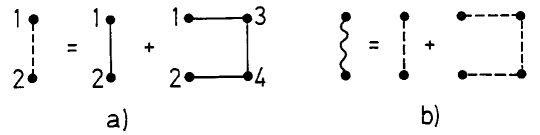
Figure 2: Fuzzing. In a) the solid line 12-link is replaced by the dashed line 12-link.
In b) this dashed line 12-link is itself now replaced by the wavy line 12-link.

This illustrates the replacement

$$U^{0}_{\mu}(n)\rightarrow U^{1}_{\mu}(n)=A^{1}_{n}\Biggl{[}cU^{0}_{\mu}(n)+\sum_{\stackrel{{\scriptstyle\pm\nu\not=\mu}}{{\nu\not=4}}}U^{0}_{\nu}(n)U^{0}_{\mu}(n+\bar{\nu})U^{0{\dagger}}_{\nu}(n+\bar{\mu})\Biggr{]}$$ (0.18)

to give links $U^{1}$ constructed from the basic links $U^{0}$ by a single fuzzing $j=1$. This is followed by

$$U^{1}_{\mu}(n)\rightarrow U^{2}_{\mu}(n)=A^{2}_{n}\Biggl{[}cU^{1}_{\mu}(n)+\sum_{\stackrel{{\scriptstyle\pm\nu\not=\mu}}{{\nu\not=4}}}U^{1}_{\nu}(n)U^{1}_{\mu}(n+\bar{\nu})U^{1{\dagger}}_{\nu}(n+\bar{\mu})\Biggr{]}$$ (0.19)

to give links $U^{2}$ constructed from the $U^{1}$ by a second fuzzing $j=2$ and so on. In general

$$U^{m-1}_{\mu}(n)\rightarrow U^{m}_{\mu}(n)=$$

$$A^{m}_{n}\Biggl{[}cU^{m-1}_{\mu}(n)+ \sum_{\stackrel{{\scriptstyle\pm\nu\not=\mu}}{{\nu\not=4}}}U^{m-1}_{\nu}(n)U^{m-1}_{\mu}(n+\bar{\nu})U^{m-1\ {\dagger}}_{\nu}(n+\bar{\mu})\Biggr{]}.$$ (0.20)

Here the $A^{j}_{n}$ are normalisation factors chosen to project the $U^{j}_{\mu}(n)$ into $SU(N_{C})$ and $c$ is, in principle, a free parameter. However, experience when measuring energies [90, 91] has shown for SU(2) that $c=4$ is a suitable value for the present class of problems. The value of $c$ could be optimized, but it is found that results are never crucially dependent on the precise value of $c$. Another degree of freedom is the amount of fuzzing ($m$). For correlations over large distances the greater the fuzzing the better the efficiency of the calculation in the sense that the state $\Psi(Q\bar{Q})$ in Eq. 0.11, generated by connecting together a series of fuzzed links, is expected to have a greater overlap with the true ground state wave function. In some cases this has been carried to great lengths e.g. in Ref. [92] $m=$110 fuzzing iterations were used, since there the emphasis was on quark separations upto 24 lattice spacings.

In the calculation of the interquark potential in Eq. 0.15, the fuzzing procedure plays the second rôle of generating different paths ($P_{i}$) between quarks, for use in the variational approach of Ref. [90, 91]. In this notation the basic path from Eq. 0.11 is $P_{0}=U^{0,ab}U^{0,bc}U^{0,cd}.....U^{0,za}$ and the fuzzed paths $P_{i}=U^{i,ab}U^{i,bc}U^{i,cd}.....U^{i,za}$ . The variational approach then yields the correlation matrix between paths with different fuzzing levels $i,j$

$$W^{t}_{ij}=<P_{i}|\bar{T}^{t}|P_{j}>.$$ (0.21)

Here $\bar{T}=\exp(-a\bar{H})$ is the transfer matrix for a single time step $a$, with the basic QCD Hamiltonian $\bar{H}$, the $P_{i,j}$ are paths constructed as products of fuzzed basic links and, as before, $t$ is the number of steps in the imaginary time direction. As shown in Ref. [90, 91], a trial wave function $\psi=\sum_{i}a_{i}|P_{i}>$ leads to the eigenvalue equation

$$W^{t}_{ij}a^{t}_{j}=\lambda^{(t)}W^{t-1}_{ij}a^{t}_{j}.$$ (0.22)

For a single path this reduces to

$$\lambda^{(t)}=\frac{W^{t}_{11}}{W^{t-1}_{11}}=\exp(-aV_{Q\bar{Q}}),$$ (0.23)

where $V_{Q\bar{Q}}$ is the potential of the quark system being studied. Unfortunately, in this single path case i.e. with only $P_{0}$ as in the previous subsection, $t$ needs to be large and this can lead to unacceptable error bars on the value of $V_{Q\bar{Q}}$ extracted. However, if — in addition — a few fuzzed paths are included, it is found that $t$ need only be small $(t\approx 5)$ to get a good convergence to $V_{Q\bar{Q}}$ with small error bars.

A further very important advantage of fuzzing is that not only can the lowest eigenvalue be extracted but also higher ones, since a matrix diagonalisation is involved. These higher states correspond to excitations of the gluon field. However, with the direct paths from the $Q$ to $\bar{Q}$ in Eq. 0.12, these excitations are purely S-wave. To generate non-S-wave gluonic excitations combinations of indirect paths are needed — see Chapter 2.

The above fuzzing is an attempt to improve the overlap of the lattice wavefunction with the true ground state wavefunction and so only involves spatial links (N.B. $\nu\not=4$ in the summations in Eq. 0.18 i.e. the staples in Fig. 2 are purely spatial). However, a similar procedure can be applied to a time-like link [93]. In the notation of Eq. 0.18, the basic time-like link $U^{0}_{\mu=0}(n)$ is now replaced by $W^{0}_{\mu=0}(n)$ — the average of the six staples in the planes $(\pm x,T),\ (\pm y,T)$ and $(\pm z,T)$. The benefit gained from this is a reduction in the Noise/Signal ratio $R_{{\rm NS}}$ for configurations involving a static quark. Without this time-like fuzzing, it has been observed for $B$-meson correlations, with time extent $x_{0}$, that $R_{{\rm NS}}\propto\exp(x_{0}\Delta E)$, where $\Delta E=E_{0}-m_{\pi}$ with $E_{0}$ being the ground state energy of the $B$-meson [94]. This leads to very noisy signals as $x_{0}$ increases. However, using $W^{0}_{\mu=0}(n)$ results in almost an order of magnitude reduction in $R_{{\rm NS}}$ for $x_{0}\approx 1.5$ fm. This is shown in Fig. 3.

Figure 3: Noise to signal ratio ($R_{{\rm NS}}$) of a $B-$meson correlation function as a function of the time extent $x_{0}$. The solid dots are when using simply $U^{0}_{\mu=0}(n)$. The open squares are for $W^{0}_{\mu=0}(n)$ and the open triangles for $W_{{\rm HYP}}$ [93].

An even greater reduction in $R_{NS}$ can be achieved, if the single staple fuzzing in Fig. 2 is replaced by the hypercubic blocking of Ref. [95]. There each level of fuzzing is described by three equations (and so needing three free parameters $c_{i}$) similar to Eq. 0.18. But these three equations mix links that are connected to the original link only i.e. this “fuzzing” only involves links in the hypercube defined by the original link. This procedure yields a fuzzed link $W_{{\rm HYP}}$ that is much more local than three fuzzing levels from Eq. 0.18 and so preserves short distance spatial structure. Furthermore, when this is applied to a time-like link, then it reduces $R_{{\rm NS}}$ even further than the use of $W^{0}_{\mu=0}(n)$. The use of hypercubic links is still in its infancy and we should expect to see much more of this development in the future — see Refs. [96]. This is also shown in Fig. 3.

2 Lattice calculations with $[(Q\bar{Q})(Q\bar{Q})]$ configurations

The previous section outlines the techniques for extracting the two-quark potential. This is now generalised to the $[(Q\bar{Q})(Q\bar{Q})]$ case, where the quarks are on the corners of a rectangle with sides of length $d$ and $r$. During the Monte Carlo simulation, the correlations $W_{ij}(r)$ in Eq. 0.21 — appropriate for extracting the two-quark potential $V_{{Q\bar{Q}}}(r)$ — and the correlations $W_{ij}(d,r)$ for the four-quark potential $V_{4}(d,r)$ are evaluated at the same time. As an example, in Ref. [86] for $W_{ij}(r)$ three paths were generated by the three different fuzzing levels $m=$12, 16 and 20. On the other hand, for the $W_{i^{\prime}j^{\prime}}(d,r)$ only the level 20 was kept, with the variational basis $(i^{\prime}j^{\prime})$ being the two configurations $A$ and $B$ in Figs. 4.

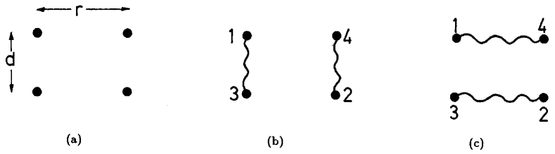
Figure 4: a) Four quarks in a rectangle of sides $r$ and $d$:
The two partitions b) $A=[Q_{1}\bar{Q}_{3}][Q_{2}\bar{Q}_{4}]$ and c) $B=[Q_{1}\bar{Q}_{4}][Q_{2}\bar{Q}_{3}]$

These lead to the Wilson loops in Fig. 5.

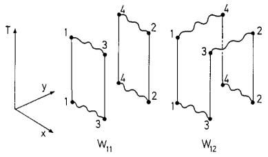
Figure 5: The 4-Q Wilson loops $W_{11}$ and $W_{12}$.

In the case of squares (i.e. $r=d$), Eq. 0.22 gives the potential energy of the ground state as

$$E_{0}= aV_{4}(d,d)=aE_{4}(d,d)-2E(d)$$

$$= \log\left[\frac{W_{11}^{t-1}(d,d)+W_{12}^{t-1}(d,d)}{W_{11}^{t}(d,d)+W_{12}^{t}(d,d)}\right]-2E(d)$$ (0.24)

and that of the first excited state

$$E_{1}=\log\left[\frac{W_{11}^{t-1}(d,d)-W_{12}^{t-1}(d,d)}{W_{11}^{t}(d,d)-W_{12}^{t}(d,d)}\right]-2E(d),$$ (0.25)

where $E(d)$ is the result of diagonalising the $3\times 3$ variational basis for $V_{Q\bar{Q}}$. In these equations, $t$ should tend to $\infty$. However, in practice it is found to be sufficient to have $t\approx 5$ for extracting accurate values for $E_{0}$ and $E_{1}$.

The results are shown in Fig. 6.

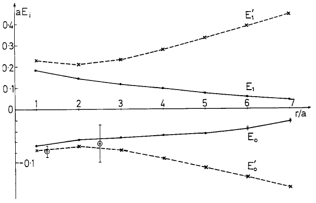
Figure 6: The comparison of the lattice data $E_{0,1}$ (continuous line) with the $f=1$ model results $E^{\prime}_{0,1}$ (dashed line) in Subsec. 1 — see Ref. [87]. Also the two lattice data points from Ref. [97] are included.

For comparison this also includes the corresponding 1985 results of Ref. [97] as the two points with large error bars at $r/a\approx 1.25$ and 2.5 — remembering that the lattice spacing for Ref. [97] is $a^{\prime}\approx 0.15$fm $\approx 1.25a$, where $a\approx 0.12$ fm from Ref. [87]. It is seen that the present calculation gives energies that have error bars which only become significant for $r/a\geq 7$, whereas the 1985 work was unable to generate any meaningful numbers beyond $r/a^{\prime}=2$. In fact, for the present purpose, neither of the 1985 points is of use, since the $r/a^{\prime}=1$ result could well suffer from lattice artefacts — a problem afflicting all calculations of configurations involving a single lattice spacing — and the $r/a^{\prime}=2$ result has error bars that are too large for the analysis in Subsec. 5 to be carried out. However, the following should be added in defence of Ref. [97]. Firstly, their calculation was for SU(3) and so it was, at least, an order of magnitude more demanding on CPU time — especially in 1985. Secondly, it should be remembered that the energies of interest ($E_{0,1}$) are very small compared with the total four-quark energy $E_{4}$ in Eq. 2. For example, at $r=d=4a$ the value of $aE_{0}=-0.050(1)$ is obtained from the difference between $aE_{4}$ and $2aE(d)$, which is 1.505–1.555 i.e. the error quoted on $aE_{0}$ is less than $0.1\%$ of $aE_{4}$.

One of the most outstanding features of the results is that for $r$ equals $d$ the value of $aE_{0}$ decreases smoothly in magnitude from –0.07 for $r=d=a$ to –0.04 for $r=d=6a$. However, for the few cases where $r\not=d$ the value of $E_{0}$ is an order of magnitude smaller than the adjacent $r=d$ cases e.g. $E_{0}(2,3)\approx-0.006$, whereas $E_{0}(2,2)$ and $E_{0}(3,3)$ are $\approx-0.055$. This result is reminiscent of the conclusion found with the flux-tube model [98] and the ansatz made in the flip-flop model of Refs. [89]. In both of these models the interaction between the two separate two-quark partitions of Fig. 4 is very small (in fact zero in the flip-flop model) except when the unperturbed energies of the two partitions is the same i.e. at $r=d$ in the case of rectangles.

3 Lattice parameters and finite size/scaling check

Most of the above (and later) calculations involving only static quarks were carried out with the parameters in Table 2. There the coupling $\beta$ is defined after Eq. 0.17 and the lattice spacings $a_{n}$ were determined by, for example, the Sommer method described in Subsec. 1. Each of these three sets serve a specific purpose.

Benchmark data

Set 1 shows the original parameters with which most calculations are performed (e.g. for the results in Fig. 6) and against which the following results with Sets 2 and 3 are compared. These parameters are chosen so that — unlike Sets 2 and 3 — the problems of computer memory and CPU time do not prevent generating many “independent” measurements to ensure good error estimates.

Finite size effect

Table 2: Typical SU(2) lattice parameters used in $[(Q\bar{Q})(Q\bar{Q})]$ calculations. Much of the notation is explained in the text with M/G being the number of Measurements per Geometry.

Set	$L^{3}\times T$	$\beta$	$a_{n}$ (fm)	M/G	Refs.
1	$16^{3}\times 32$	2.4	$\approx 0.12$	720	[86]–[88]
2	$24^{3}\times 32$	2.4	$\approx 0.12$	160	[88]
3	$24^{3}\times 32$	2.5	$\approx 0.082$	660	[88]

With Set 2 the effect of the finite lattice size is checked. However, in the present case it was found that the results for the size of squares considered (i.e. up to $7\times 7$) were unchanged within error bars — see Table 2 in Ref. [88]. This type of check is important for large squares because of the spatial periodic boundary conditions at $0$ and $L$. Two quarks can be connected by two paths — a direct path on the lattice (e.g. that in Eq. 0.12) or an indirect path that encircles the boundary. If the two quarks are separated by $r>L/2$, then the indirect path is of length $L-r<r$ and so is potentially more important than the direct path — the only one of the two that is explicitly treated. In the present case with $L=16$, such problems should only begin to occur seriously with $8\times 8$ squares. For this larger lattice, fewer configurations per square were generated, since the storage and computer time increased by about a factor of $\approx(24/16)^{3}\approx 3.$

Smaller lattice spacing

In most cases the possible importance of finite size effects can be seen beforehand by using simple arguments. We know, for example, that the length $r$ of the direct path should be smaller than the length $L-r$ of the indirect path. However, the effect as $a\rightarrow 0$ is not obvious and needs checking. In order to isolate this scaling effect from the finite size effect, it is convenient to use lattices that have approximately the same physical size. Therefore, since the spatial volume for Set 1 is $(16\times 0.12)^{3}\approx 7$ fm³, the value of $a_{3}$ for a $24^{3}$ lattice should be $\approx 7^{1/3}/24\approx 0.08$ fm — a lattice spacing that corresponds to $\beta\approx 2.5$. For the results to show scaling, the physical energies (i.e. in, say, MeV) at the same values of $r$ (in fm) should be the same. In this case, it means

$$E[{\rm Set}\ 1\ ({\rm or}\ 2),\ r/a_{1}]\approx E[{\rm Set}\ 3,\ r/a_{3}],$$ (0.26)

where the $a_{n}$E(Set n, $r/a_{n}$) are the dimensionless numbers given by the lattice calculations and the $r/a_{n}$ are the number of lattice links between the quarks. Of course, in general only $r/a_{1}$ or $r/a_{3}$ is an integer, so that the comparison in Eq. 0.26 must be done by interpolation. This approximate equality is sufficiently well satisfied in the present problem (see Table 3 in Ref. [88]). In Ref. [49] a more complete test of the $a\rightarrow 0$ limit is carried out with the addition of the non-rectangular geometries to be discussed in Sec. 6. There the $\beta$ values (and lattice sizes) used were $\beta$= 2.35, 2.4 ($16^{3}\times 32)$, 2.45 ($20^{3}\times 32)$, 2.5 ($24^{3}\times 32)$ and 2.55 ($26^{3}\times 32)$ and led to 4-quark energies that were essentially independent of $a$ over this range of $\beta$ i.e. scaling was achieved for $\beta\geq 2.35$.

It should be added that the above procedure is called scaling in contrast to asymptotic scaling. The latter relates results from different values of $a(\beta)$ by perturbative arguments and is not expected to apply at the comparatively large values of $a$ in Table 2 — see Ref. [99].

5 Potential Model Description of the Lattice Data

The assumption often made by those who create models for multi-quark systems is that these systems can be treated in terms of two-body potentials. This is the Nuclear Physics inspired approach that is very successful for, say, multi-nucleon systems, where three- and four-body forces are small. Of course, the fact that the latter were small was at first simply an assumption. However, later this was found to be justified by Weinberg [23] using various low-energy theorems that force the $\pi N\rightarrow\pi N$ interaction — the main mechanism for multi-nucleon forces — to essentially vanish in nuclei. At present, there seems to be no such simplifying feature for multi-quark interactions. In the following, I will first show the consequences of using — in the four-quark system — simply two-quark potentials unmodified by the presence of the other two quarks. Then this model will be improved by including also a direct four-quark interaction. These are examples of what was referred to as Effective Potential Theories (EPTs) in Subsec. 2. However, since the quarks are now static, there is no kinetic energy and so the question of which quark wave equation to use does not arise. Similarly, the effective quark masses do not enter, since the quantities of interest are the binding energies between the two 2-quark clusters. Therefore, of the three ingredients usually needed for an EPT of Subsec. 2 only freedom with the interquark potential remains. This is both a weakness, by being a model that is unrealistic and not comparable with any experimental data — except for possible future $\Upsilon(b\bar{b},9.5{\rm GeV})\Upsilon(b\bar{b},9.5{\rm GeV})$ scattering — and a strength, in that only the potential ingredient plays a rôle.

1 Unmodified two-body approach

Once the quark–quark potential $V_{Q\bar{Q}}$ is known and, if it is assumed to be the only interaction between the quarks, then the energy of a multi-quark system can be readily calculated — provided the wave function for that system is expressed in terms of a sufficient number of basis states. For the present situation, the most obvious choices for such states are $A$ and $B$ in Figs. 4 b) and c).

In this extreme two-body approach, since the presence of the gluon fields have been explicitly removed — their only effect now being in the colour indices of the quarks — the states $A$ and $B$ form a complete but non-orthogonal basis. This implicitly assumes in Figs. 4 the quark $(Q)$, antiquark $(\bar{Q})$ assignment $A=[Q_{1}\bar{Q}_{3}][Q_{2}\bar{Q}_{4}]$. In SU(2) the other quark assignment $[Q_{1}Q_{3}][\bar{Q}_{2}\bar{Q}_{4}]$ is numerically equivalent and so leads to nothing new. In this approach, states are excluded in which the gluon fields are excited. However, later this restriction is relaxed in an extension to the model in Sec. 7 and Appendix A.3. The energies ($E^{\prime}_{i}$) of this static four-quark system can be extracted from the eigenvalues of the Hamiltonian

$$\left({\bf V}-\lambda_{i}{\bf N}\right)\Psi_{i}=0,$$ (0.27)

where the normalisation matrix

$${\bf N}=\left(\begin{array}[]{cc}1&1/2\\ 1/2&1\end{array}\right)$$ (0.28)

and the potential energy matrix

$${\bf V}=\left(\begin{array}[]{cc}v_{13}+v_{24}&V_{AB}\\ V_{BA}&v_{14}+v_{23}\end{array}\right).$$ (0.29)

Several points need explaining in these equations.

1. The off-diagonal matrix element $N_{12}=\langle A|B\rangle=1/2$ shows the non-orthogonality of the $A,B$ basis. In general, for SU($N_{C}$) this becomes $N_{12}=1/N_{C}$ and arises simply by recoupling the colour components of the quark terms i.e.

   $$|1_{1\bar{4}}1_{2\bar{3}}\rangle=\frac{1}{N_{C}}|1_{1\bar{3}}1_{2\bar{4}}\rangle+\frac{\sqrt{N_{C}^{2}-1}}{N_{C}}|A_{1\bar{3}}A_{2\bar{4}}\rangle,$$ (0.30)

   where $|1_{i\bar{j}}\rangle$ and $|A_{i\bar{j}}\rangle$ are the SU($N_{C}$) singlet and adjoint representations.

   At this stage, the lack of orthogonality could have been avoided by simply using the basis $A\pm B$. However, later it will be seen that the $A,B$ basis is in fact more convenient and suggestive, when the gluon fields are reintroduced in a more explicit manner.

2. The interquark potential $V_{Q\bar{Q}}(ij)=v_{ij}$ in Eq. 0.6 has been extracted as the potential energy between a single static quark ($Q$) and a single static antiquark ($\bar{Q}$). In order to evaluate general multiquark potential energy matrix elements, a further assumption is needed concerning the colour structure of $v_{ij}$. Here the usual identification

   $$V_{ij}=-\frac{1}{3}{\bf\tau}_{i}.{\bf\tau}_{j}v_{ij}$$ (0.31)

   will be made, where the ${\bf\tau}_{i}$ are the Pauli spin matrices appropriate for SU(2). This choice ensures, for a colour singlet meson-like state $[ij]^{0}$, that $\langle[ij]^{0}|{\bf\tau}_{i}.{\bf\tau}_{j}|[ij]^{0}\rangle=-3$ and

   $$\langle[ij]^{0}|V_{ij}|[ij]^{0}\rangle=v_{ij}.$$ (0.32)

   Strictly speaking, the form in Eq. 0.31 is only true in the weak coupling limit of one-gluon exchange, since this has replaced the local gauge invariance — ensured by the series of $U$-links of Eq. 0.11 connecting the two quarks — by the global gauge invariance reflected by the ${\bf\tau}_{i}.{\bf\tau}_{j}$ factor.

3. With the choice of $V_{ij}$ in Eq. 0.31, the off-diagonal potential matrix element becomes

   $$\langle A|V|B\rangle= V_{AB}=V_{BA}$$

   $$= \frac{1}{2}\left(v_{13}+v_{24}+v_{14}+v_{23}-v_{12}-v_{34}\right).$$ (0.33)

   Since the following discussion only involves quark configurations in the rectangular geometries of Figs. 4, it is convenient to use the notation

   $$v_{13}=v_{24}=v_{d},\ \ v_{14}=v_{23}=v_{r}\ \ {\rm and}\ \ v_{12}=v_{34}=v_{x},$$ (0.34)

   where the suffix $x$ refers to the diagonals of the rectangles in Fig. 4.

Even though the form of Eq. 3 is derived in the one-gluon exchange limit, it is now assumed that a more realistic model emerges if the $v_{ij}$ are taken to be the complete potential of Eq. 0.6 and not just the one-gluon exchange component. This clearly has the correct form when the distance between the two two-quark clusters of Fig. 4 are far apart, since in this case the only interactions are those within the separate clusters — due to the cancellation in Eq. 3 of $v_{12},\ v_{34}$ with either $v_{13},\ v_{24}$ or $v_{14},\ v_{23}$.

The $2\times 2$ Hamiltonian of Eq. 0.27 is easily diagonalised to give the eigenvalues $\lambda_{0,1}$. Since it is the binding energy $E^{\prime}_{i}$ of the four-quark system that is of interest, and also that was extracted in Subsec. 2 from the Monte Carlo simulation, the internal energy of the meson-like state with the lowest energy (i.e. $2v_{d}$ for $d\leq r$) is now subtracted from the $\lambda_{i}$ to give

$$E^{\prime}_{i}=\lambda_{i}-2v_{d}$$ (0.35)

in analogy with the lattice expressions in Eqs. 2 and 0.25.

Therefore, in this simplest version of the two-body approach, the $E^{\prime}_{i}$’s should correspond to the $E_{i}$’s from the Monte Carlo simulation — a comparison which is made in Fig. 6. Since the values of $E_{0}$ for squares (i.e. $r=d$) are much larger than those for neighbouring rectangles, only the results for squares are shown in Fig. 6. In these cases

$$E^{\prime}_{0}=-\frac{2}{3}(v_{x}-v_{d})\ \ {\rm and}\ \ E^{\prime}_{1}=2(v_{x}-v_{d})=-3E^{\prime}_{0},$$ (0.36)

In addition, the corresponding normalised wave functions are of the form $\psi(E^{\prime}_{0})=\frac{1}{\sqrt{3}}|A+B\rangle$ and $\psi(E^{\prime}_{1})=|A-B\rangle$.

Two comments should be made on these results:

• For the smallest squares and rectangles the agreement between $E_{i}$ and $E^{\prime}_{i}$ is best. This is reasonable, since it is expected that at small interquark distances perturbation theory is adequate i.e. the lowest order gluonic effects are already incorporated correctly into the interquark potential.

• As the squares and rectangles get larger the differences between the $E_{i}$ and the $E^{\prime}_{i}$ grow until $E^{\prime}_{0}$ is more than three times $E_{0}$, and $E^{\prime}_{1}$ more than seven times $E_{1}$, for the largest squares $d\approx 7a\approx 0.8$ fm. Since $E^{\prime}_{0}$ is too attractive and $E^{\prime}_{1}$ too repulsive, this suggests that the off-diagonal matrix element $V_{AB}$ in Eq. 3 is too large.

The main conclusion to be drawn from the above is that the two-body potential of Eq. 0.31 does not give the potential energy of the four-quark system — the indication being that the off-diagonal potential energy $V_{AB}$ is too large. This is nothing more than the well known van der Waals effect of Ref. [100] — see Oka and Yazaki in Chapter 6 of Ref. [36].

2 The effect of multiquark interactions

In the above model it is assumed that all of the gluonic effects are incorporated into the two-body potential $v_{ij}$. However, this is clearly an oversimplification that is at best only applicable in situations where perturbation theory holds, namely at short distances, as already noted in the discussion of Fig. 6. In more realistic models, the QCD coupling is sufficiently strong to constrain the gluon field into flux-tubes connecting the quarks in a given meson — as visualised by the wavy lines between the quarks in states $A$ and $B$ in Figs. 4. Therefore, the overlap of states $A$ and $B$, i.e. $N_{12}=\langle A|B\rangle$, is not simply the colour recoupling factor of 1/2, but should also involve the lack of overlap of the gluon fields in states $A$ and $B$. This can be incorporated by introducing an entity $f$, which simply multiplies the original $N_{12}$, and which is an unknown function of the position coordinates of the four quarks. With this interpretation of $f$ as a gluon field overlap factor, it is also necessary to multiply the off-diagonal potential matrix element $V_{AB}$ of Eq. 3 by the same factor $f$. This factor must be the same in $N_{12}=f/2$ and $V_{12}=fV_{AB}$, since otherwise the binding energies $E^{\prime}_{0,1}$ would be dependent on the self-energy term $c$ in the form of $v_{ij}$ given in Eq. 0.6 — which would be unphysical. The $E^{\prime}_{0,1}$ are now extracted from Eq. 0.35 after diagonalising

$$\left[{\bf V}(f)-\lambda_{i}(f){\bf N}(f)\right]\Psi_{i}=0$$ (0.37)

with

$${\bf N}(f)=\left(\begin{array}[]{cc}1&f/2\\ f/2&1\end{array}\right)\ \ {\rm and}\ \ {\bf V}(f)=\left(\begin{array}[]{cc}v_{13}+v_{24}&fV_{AB}\\ fV_{BA}&v_{14}+v_{23}\end{array}\right).$$ (0.38)

The two equations (0.37) and (0.38) are the basis of the following analysis. They give a procedure for extending the model of Eqs. 0.27 – 0.29, which was justified in the weak coupling limit, into the domain beyond one-gluon exchange. The off-diagonal potential matrix element performs this extension in two ways. Firstly, even though $V_{AB}$ in Eq. 3 still has the same algebraic structure in terms of the $v_{ij}$ as dictated by the one-gluon exchange limit, the $v_{ij}$’s themselves are the full two-quark potential of Eq. 0.6. Secondly, in the off-diagonal correlation $W_{12}$ of Fig. 5, the one-gluon exchange model suggests the presence of the overall multiplicative factor $f$ due to gluon exchange within the initial and final states $A$ and $B$ at euclidean times $T=0$ and $\infty$. In this interpretation, the terms in $V_{AB}$ arise during the period of propagation between $T=0$ and $\infty$.

The strategy is now to adjust $f$ to get an exact fit to $E_{0}$ or $E_{1}$. In the case of squares, since

$$E^{\prime}_{0}=\frac{-f}{1+f/2}(v_{x}-v_{d})\ \ {\rm and}\ \ E^{\prime}_{1}=\frac{f}{1-f/2}(v_{x}-v_{d}),$$ (0.39)

the appropriate expressions are

$$f(E_{0})=\frac{E_{0}}{v_{d}-v_{x}-E_{0}/2}\ \ {\rm and}\ \ f(E_{1})=\frac{E_{1}}{-v_{d}+v_{x}+E_{1}/2}$$ (0.40)

for fitting $E_{0}$ and $E_{1}$ respectively — the results being shown in Fig. 7. For general rectangles the corresponding equations are somewhat more complicated.

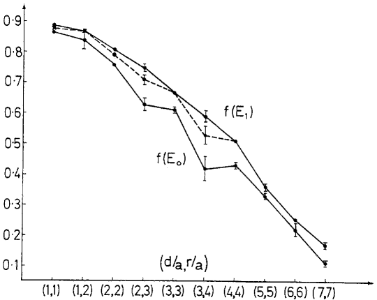
Figure 7: The values of $f(E_{0})$, $f(E_{1})$ and $\bar{f}$ (from Subsec. 3).

Two points should be noted from this figure:

• All values of $f$ are less than unity as is expected from the interpretation of $f$ as a gluon field overlap factor. In addition, this idea is supported by the fact that the values of $f$ decrease as the quarks get further apart.

• The values of $f(E_{0})$ and $f(E_{1})$ are rather similar, which suggests that a compromise value of $f$ would give a reasonable description of both $E_{0}$ and $E_{1}$ — as will be seen below.

3 A compromise for the overlap factor $f$

The previous subsection suggests that for each geometry a single value of $f$ could give a reasonable description of both $E_{0}$ and $E_{1}$. Here one such possibility is given by finding that value of $\bar{f}$ which minimizes the expression

$$D(\bar{f})=\left(\frac{E_{0}-E^{\prime}_{0}(\bar{f})}{\Delta E_{0}}\right)^{2}+\left(\frac{E_{1}-E^{\prime}_{1}(\bar{f})}{\Delta E_{1}}\right)^{2},$$ (0.41)

where the $\Delta E_{i}$ are the errors quoted for the $E_{i}$ from the lattice calculation. The result is shown by the dashed line in Fig. 7.

It is seen that indeed a single value of $f=\bar{f}$ suffices to explain reasonably well both energies. This is a non-trivial observation, since it indicates that the parametrization suggested in Eqs. 0.37, 0.38 contains the most important features of the more precise lattice calculation.

It should be added that the extraction of a compromise value of $f$ is not simply a curiosity, since any model that needs different values of $f$ for $E_{0}$ and $E_{1}$ would be more difficult to use in practice for more complicated multi-quark systems.

At this point, even though for each geometry a single value of $f=\bar{f}$ gives values of $E^{\prime}_{0,1}$ that are in reasonable agreement with the $E_{0,1}$, it might be asked about the remaining small differences. Several possibilities are now open:

• The lattice energies $E_{i}$ may not be sufficiently accurate due to finite lattice size and scaling uncertainties. This was checked in Ref.[88] and found not to be a problem.

• The parametrization in Eqs. 0.37, 0.38 may be inadequate. One possibility would be to combine the notion of a gluon overlap factor $f$ with a generalized form for the two-quark potential in Eq. 0.6, since this could introduce more free parameters.

• Any model based only on states $A$ and $B$ in Fig. 4 is incomplete and other states are necessary in addition. This point will be discussed further in Sec. 7.

• The step from Eq. 0.27 to Eq. 0.37 was motivated by one gluon exchange. However, this could possibly be extended by performing a two-gluon exchange calculation to see what new terms arise and to then be guided by this in making an improved parametrization — the topic of the next subsection.

4 The effect of two-gluon exchange

In Ref. [101] it was noted that the two-body $f=1$ models discussed in Subsec. 1 correspond to lowest order perturbation theory in the quark–gluon coupling i.e. to order $\alpha=g^{2}/4\pi$ in the notation of Eq. 0.17. This was extended in Ref. [102], where a perturbative calculation to fourth order in the quark–gluon coupling (i.e. to $O(\alpha^{2})$) was made for the potential of the $QQ\bar{Q}\bar{Q}$ system. This was performed in the general case of colour SU($N$). Considering the quarks to be at points $R_{i}$ define

$$V_{A}=V(R_{13})+V(R_{24}),\ V_{B}=V(R_{14})+V(R_{23}),\ V_{C}=V(R_{12})+V(R_{34}),$$

where $V(R_{pq})$ is the two-body potential between the different quark and antiquark pairs a distance $R_{pq}$ apart. For the two possible energy eigenstates, diagonalization yields the following two potentials correct to $O(\alpha^{2})$:

$$V_{0}=$$

$$\frac{\left(N^{2}\!-\!2\right)\left(V_{A}\!+\!V_{B}\right)+2V_{C}-N\sqrt{N^{2}\left(V_{A}\!-\!V_{B}\right)^{2}+4\left(V_{A}\!-\!V_{C}\right)\!\left(V_{B}\!-\!V_{C}\right)}}{2\left(N^{2}-1\right)}$$

$$V_{1}=$$

$$\frac{\left(N^{2}\!-\!2\right)\left(V_{A}\!+\!V_{B}\right)+2V_{C}+N\sqrt{N^{2}\left(V_{A}\!-\!V_{B}\right)^{2}+4\left(V_{A}\!-\!V_{C}\right)\!\left(V_{B}\!-\!V_{C}\right)}}{2\left(N^{2}-1\right)}.$$ (0.42)

These potentials are exactly equal to those given by the naive ($f=1$) two-body model in Eqs. 0.27 – 0.29. This fact that a straightforward two-body model is correct also to next-to-leading order in the quark–gluon coupling may be surprising in light of the non-abelian nature of QCD. However, Ref. [102] does go on to show that this two-body model fails at $O(\alpha^{3})$ as three- and four-body forces appear due to the onset of three-gluon vertex effects. In general, their nature seems to be complicated, but for some geometries simplifications are possible; e.g. for the four quarks on the corners of a regular tetrahedron there will be no contribution from quark self–interactions to four-body forces to $O(\alpha^{3})$.

The overall conclusion from Ref. [102] is as follows: “Looking at the Monte Carlo lattice calculations for the $QQ\bar{Q}\bar{Q}$-system in Refs. [87, 88], it is observed that for small interquark distances of a few lattice spacings (with $a\approx 0.12$ fm) the $f=1$ two-body model gives a reasonable approximation in the sense that the four-quark potentials calculated from Eq. 0.42 using the Monte Carlo two-body potentials are comparable to the four-quark potentials from the lattice simulation. The agreement improves the smaller the distances get. By comparing the perturbative (i.e. $1/R$) and non-perturbative (i.e. linear) part in the usual parametrization of the $Q\bar{Q}$-potential in Eq. 0.6, one would expect to start entering the perturbative regime when distances get down to about two lattice spacings. However, at that stage the approximation provided by the two-body model is already very good. The fact that the two-body model is correct to fourth order in perturbation theory certainly suggests that it should be a reasonable approximation in the perturbative domain. This result supports the belief that the results of the lattice simulations for small enough distances indeed are correlated to continuum perturbation theory, and thus that continuum physics is extracted from the Monte Carlo calculations.”

So far in this section various models have been proposed in an attempt to understand the results of the Monte Carlo simulations of lattice QCD. The main outcome — summarised in Fig. 7 — is the emergence of a function $\bar{f}$ that depends on the coordinates of the four quarks involved. This shows that the usual models based on purely two-quark interactions need to be modified considerably — essentially by the factor $\bar{f}$, which becomes $\ll 1$ for large interquark distances. This observation is in itself of much interest, but at this stage it is not clear how the effect can be incorporated into more realistic situations in which the quarks are not so restricted in their geometry. It is the purpose of the next section to tackle this problem by first studying how $\bar{f}$ can be parametrized.

5 Parametrizations of the gluon-field overlap factor $f$

In Subsecs. 2, 3, models were introduced in an attempt to understand the ground state binding energy $(E_{0})$ and excited state energy $(E_{1})$ emerging from a Monte Carlo simulation, in which four quarks were at the corners of a rectangle. These models are summarised by Eqs. 0.37, 0.38. For each quark configuration, both of the energies $E_{0,1}$ are described in terms of a function $f$ of the four quark positions — Eq. 0.39. As it stands, this is not particularly useful, when wishing to extend these ideas to systems containing more than four quarks, unless $f$ can be parametrized in some sensible and convenient manner. In the literature, several parametrizations have been suggested. In Refs. [101, 103], motivated by strong coupling arguments, the phenomenological form is taken to be

$$f_{1}=\exp[-\alpha b_{s}S],$$ (0.43)

where $b_{s}=0.0736$ is the string tension in the interquark potential of Eq. 0.6 and $S$ is the minimal area of the surface bounded by the straight lines connecting the quarks and antiquarks. The other form, the one proposed in [104], is

$$f_{2}=\exp\big{[}-\frac{kb_{s}}{6}\sum\limits_{i<j}r^{2}_{ij}\big{]}$$ (0.44)

i.e. the cut-down is governed by the average of the six links present in a $Q^{2}\bar{Q}^{2}$ system. In Eqs. 0.43, 0.44 the $\alpha$ and $k$ are at present free parameters to be determined later. Both of these parametrizations of $f$ accommodate the following two extreme models.

• Weak coupling, which has $f=1$ when all $r_{ij}=0$. This $f=1$ limit was assumed to apply for all values of $r_{ij}$ in Subsec. 1.

• Strong coupling, which has $f=0$ when any $r_{ij}\rightarrow\infty$. In this limit the flux-tubes between the quarks in the separate mesons — seen in Fig. 4 — are then very narrow and straight. In this case the flux-tube overlap of configurations $A$ and $B$ tends to zero in the limit that any $r_{ij}\rightarrow\infty$.

With squares $(r=d)$, for which the most accurate values of $f$ exist, $k$ equals $3\alpha/4$. One measure of how meaningful these parametrizations really are, is given by extracting $\alpha$ and $k$ for each quark configuration. The hope would then be that, for squares, $\alpha$ (and therefore $k$) would be independent of the separate configurations. Only the few points for non-square rectangles $(r\not=d)$ would be able to distinguish between $f_{1}$ and $f_{2}$.

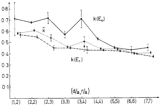
Figure 8: The values of $k(E_{0}),k(E_{1})$ and $\bar{k}$ corresponding to the values of $f(E_{0}),f(E_{1})$ and $\bar{f}$ in Fig. 7.

The outcome is depicted in Fig. 8 for the values of $k(E_{0}),k(E_{1})$ and $\bar{k}$ corresponding to the values of $f(E_{0}),f(E_{1})$ and $\bar{f}$ in Fig. 7. This shows that $k(E_{0})$ for the squares appears to decrease slowly from about 0.7 to about 0.5 as the sizes of the squares increase from ($2\times 2$) to ($7\times 7$), whereas for non-squares $k(E_{0})$ appears to be stable at about 0.7$\pm$0.1. On the other hand, $k(E_{1})$ and $\bar{k}$ decrease somewhat less and also the square and non-square values are consistent with each other.

The indications from this are that the single parameter $\bar{k}\approx 0.5(1)$ is a suitable compromise value that results in a reasonable fit to both $E_{0}$ and $E_{1}$ for a series of square and near-square geometries.

A reason for $f_{1}=\exp[-\alpha b_{s}S]$

In the limit of large $l$, Eq. 0.7 becomes

$$W(l,t)\rightarrow\exp[-tb^{\prime}_{s}l]=\exp[-b_{s}S]\ \ \ {\rm as}\ \ t\rightarrow\infty,$$ (0.45)

where $S$ is the minimal space–time area enclosed by the loop in Fig. 1. For this $Q\bar{Q}$ case, the meaning of $S$ is clear — it is simply $a^{2}lt$. But for the $[Q\bar{Q}][Q\bar{Q}]$ case in Fig. 5 the form of the appropriate minimal space–time area is less clear. However, in the extreme strong coupling limit the area $S$ is the one produced by the minimum number of elementary plaquettes needed to tile the enclosed area in question. Any fluctuations about this space-time surface would need more plaquettes and so be higher order in the strong coupling model. In this limit, the diagonal loops $W_{ii}$ in Fig. 5 are again simply two Wilson loops each tiled separately by the minimum number of plaquettes. However, the off-diagonal loops $W_{ij}$ are more complicated. A model for this was suggested in Ref. [105] and developed in Refs. [103, 106, 107]. In the notation of Fig. 9 the Euclidean Green’s function for a $Q_{A},\bar{Q}_{B},Q_{C},\bar{Q}_{D}$ system can be thought of as a $2\times 2$ matrix for a two channel problem with the $(A\bar{B})(C\bar{D})$ and $(A\bar{D})(C\bar{B})$ configurations. The transition potential between these two configurations may then be extracted from the expression for the Wilson loop of this system,

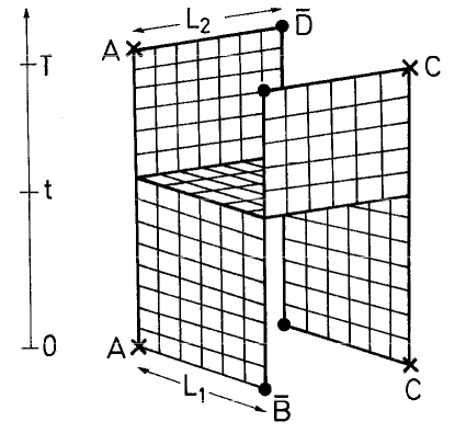
Figure 9: Tiling the transition between the states $[(Q_{A}\bar{Q}_{B})(Q_{C}\bar{Q}_{D})]$ and $[(Q_{A}\bar{Q}_{D})(Q_{C}\bar{Q}_{B})]$.

$${\bf W}(T)=\left(\begin{array}[]{cc}\exp[-2b_{s}L_{1}T]&\epsilon\\ \epsilon&\exp[-2b_{s}L_{2}T]\end{array}\right),$$ (0.46)

where $L_{1}$ and $L_{2}$ are the minimum flux tube lengths in the basis states and $b_{s}$ is the string tension of Subsec. 1. The diagonal terms are each simply the product of two propagators — $\exp[-b_{s}L_{1}T]$ for $W_{11}$ and $\exp[-b_{s}L_{2}T]$ for $W_{22}$. In a language more familiar in nuclear physics, these are simply the Green’s functions

$$W_{11}=G_{A\bar{B}}(T)G_{C\bar{D}}(T)\ \ {\rm and}\ \ W_{22}=G_{A\bar{D}}(T)G_{C\bar{B}}(T).$$ (0.47)

The mixing term

$$\epsilon=\sum_{t}\exp[-2bL_{2}(T-t)]\exp[-bL_{1}L_{2}]\exp[-2bL_{1}t]$$ (0.48)

corresponds to tiling of the off-diagonal loops $W_{ij}$. This now resembles the standard expression for the lowest order transition of a Green’s function

$$G_{fi}(T)=\int dtG_{f}(T-t)V_{fi}G_{i}(t),$$ (0.49)

where here $i,f$ denote the initial and final channels $[(Q_{A}\bar{Q}_{B})(Q_{C}\bar{Q}_{D})]$ and $[(Q_{A}\bar{Q}_{D})(Q_{C}\bar{Q}_{B})]$. Remembering that $\sum_{t}\rightarrow a^{-1}\int dt$ we can identify the transition potential as simply

$$V_{fi}=\exp[-b_{s}L_{1}L_{2}]/a\rightarrow\exp[-b_{s}S]/a$$ (0.50)

i.e. the transition potential can be expressed in terms of a spatial area — as anticipated by the models in the previous subsections. In more complicated geometries this should be the minimum area in coordinate space associated with the given boundary conditions.

6 More Complicated $[(Q\bar{Q})(Q\bar{Q})]$ Geometries

So far the only $[(Q\bar{Q})(Q\bar{Q})]$ geometries considered above were squares and rectangles. This suggested that the strongest interaction between two separate two-quark clusters occurs when the clusters are degenerate in energy — namely for square geometries compared with rectangles. To test this more, in Ref. [52] the six different geometries in Fig. 10 were studied.

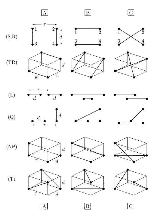
Figure 10: Six four-quark geometries a) Squares (S) and Rectangles (R), b) Tilted rectangles (TR), c) Linear (L), d) Quadrilateral (Q), e) Non-Planar (NP) and f) Tetrahedra (T). Their energies are calculated using Lattice QCD in Refs. [49, 52, 53, 86, 87, 88] and analysed in Ref. [108].

Since this confirmed that configurations degenerate in energy always gave the largest binding — not just in the square versus rectangle case — in Ref. [49] the study concentrated only on those configurations that were near degenerate.

In Ref. [53] the case of tetrahedral configurations was considered in some detail, since in SU(2) this has the three degenerate partitions seen in Fig. 10(T) when $d=r$. Since tetrahedral and linear configurations have certain interesting features, they will be discussed separately below.

However, real life is an average over all spatial configurations, so why should we be so interested in such special geometries for four static quarks? Firstly, it must be remembered that model (bridge) builders should consider all spatial possibilities — a failure with one configuration indicating that the proposed model is faulty. Also, in some ways the tetrahedral and linear configurations have simplicities and symmetries not present in other cases, which could make “Lattice QCD $\leftrightarrow$ Model” comparisons easier.

1 Tetrahedral configurations on a lattice

Since tetrahedral configurations are so symmetrical, at first sight there is no reason to consider only two of the three possible cluster partions $A+B,\ \ B+C$ or $A+C$. In this case, using the notation that the suffices $1,2,3$ are any combination of $A,B,C$ that forms a basis, then the appropriate Wilson loop matrix is [53]

$${\bf W}^{t}=\left(\begin{array}[]{ccc}W_{11}^{t}&W_{12}^{t}&W_{13}^{t}\\ W_{21}^{t}&W_{22}^{t}&W_{23}^{t}\\ W_{31}^{t}&W_{32}^{t}&W_{33}^{t}\end{array}\right).$$ (0.51)

For regular tetrahedra, the general symmetries $W_{11}^{t}=W_{22}^{t}=W_{33}^{t}$, $W_{21}^{t}=W_{12}^{t}$, $W_{31}^{t}=W_{13}^{t}$, $W_{32}^{t}=W_{23}^{t}$ are expected and, in addition, there are the equalities $W_{13}^{t}=W_{12}^{t}$ and $W_{23}^{t}=-W_{13}^{t}$. Therefore, in all, there are only two independent Wilson loops $W_{11}^{t}$ and $W_{12}^{t}$. Here the minus sign appearing in the last equation is a reminder that the quarks are in fact fermions even though quarks and antiquarks transform in the same way under SU(2). This detail is discussed more in the Appendix to Ref. [52].

Unfortunately, the inclusion of all three partitions does not lead to even more binding. However, it shows the curious feature that the ground and first excited states become degenerate in this highly symmetrical limit, since the eigenvalue equation (discussed earlier as Eq. 0.22)

$$W_{ij}^{t}a_{j}^{t}=\lambda^{(t)}W_{ij}^{t-1}a_{j}^{t},$$ (0.52)

is easily solved to give for the lowest energy (occurring twice)

$$\lambda_{1,2}=\frac{W^{t}_{11}+W^{t}_{12}}{W^{t-1}_{11}+W^{t-1}_{12}}$$ (0.53)

and for the excited state

$$\lambda_{3}=\frac{W^{t}_{11}-2W^{t}_{12}}{W^{t-1}_{11}-2W^{t-1}_{12}}.$$ (0.54)

In comparison, using only two partitions gives

$${\bf W}^{t}=\left(\begin{array}[]{ll}W_{11}^{t}&W_{12}^{t}\\ W_{21}^{t}&W_{22}^{t}\end{array}\right),$$ (0.55)

where not only is the general symmetry $W_{12}^{t}=W_{21}^{t}$ expected but also for a regular tetrahedron $W_{11}^{t}=W_{22}^{t}$. In this case Eq. 0.52 is again easily solved to give for the lowest energy

$$\lambda_{1}=\frac{W^{t}_{11}+W^{t}_{12}}{W^{t-1}_{11}+W^{t-1}_{12}}$$ (0.56)

i.e. the same as $\lambda_{1}$ in Eq. 0.53. However, for the energy of the first excited state

$$\lambda_{2}=\frac{W^{t}_{11}-W^{t}_{12}}{W^{t-1}_{11}-W^{t-1}_{12}},$$ (0.57)

which is quite different to the complete result in Eqs. 0.53, 0.54. So the degeneracy is easily explained as a feature of the more complete $3\times 3$ lattice QCD simulation. The effect is depicted in Fig. 11 as $d\rightarrow r.$ This also shows that, whereas ground state energies can be quite stable, those of excited states are more model dependent.

Figure 11: The binding energies – in units of the lattice spacing – of the four-quark states for the tetrahedral geometry of Fig. 10 (T) for $d/a=3$ and $r/a=0,1,2,3,4$.
Solid lines show lattice results: $\diamond$ – the ground-state binding energy $E_{0}$.
$\times$ – the first excited state energy $E_{1}$.
Dashed and dotted lines show model results with $f=1$ from Eqs. 0.27 – 0.29, for $E_{0}$ and $E_{1}$ respectively — see Ref [53].

The dominance of the cluster interaction by degenerate configurations was carried to the extreme in the so-called flip-flop model of Ref. [89], which makes the ansatz that the 4-quark interaction occurs only in the case of exact degeneracy. However, the model is developed for a purely linear interquark potential i.e. with only the $b_{s}$ term in Eq. 0.6, which means that the interaction only occurs when — in the notation of Fig. 4 — the spatial distances $r_{13}+r_{24}$ and $r_{14}+r_{23}$ are equal.

In several of these geometries it is not clear what is the best “natural” partition into two-quark clusters. Therefore, in the lattice simulation all three possibilities $A,\ B$ and $C$ in Fig. 10 should be taken into account. However, in some cases it is found that one (or more) of the combinations $A+B$ or $A+C$ or $B+C$ is sufficient to give — for both $E_{0}$ and $E_{1}$ — similar results to the complete $A+B+C$ simulation. This is particularly true if the configuration with the lowest energy is one of the configurations used. The study of tetrahedral and near-tetrahedral geometries on a lattice can be summarized as follows:

• From earlier work in Refs. [52, 86, 87, 88], for the corresponding squares [i.e. $(d,0)$ in Fig. 10 (T)], where two of the basis states are degenerate, the binding energy of the lowest state ranges from –0.07 to –0.05 as $d/a$ goes from 1 to 5. However, now — even though at least two of the basis states are always degenerate ($A$ and $B$) — the ground state binding energy [$E_{0}(d,r)$] is always less than that of the corresponding square [$E_{0}(d,0)$]. For a fixed $d$, $|E_{0}(d,r)|$ decreases as $r$ increases from $r=0$. Nothing interesting happens to $E_{0}$ at $r=d$, the point at which all the basis states are degenerate in energy.

• For fixed $d$, as $r$ increases from 0 to $d$, the energy of the first excited state $E_{1}$ decreases until $E_{1}(d,d)=E_{0}(d,d)$. For $r>d$, $E_{1}(d,r)$ increases again. This degeneracy of $E_{0,1}$ for the tetrahedron is a new feature compared with earlier geometries. As will emerge in Sec. 7, this is a severe constraint on models.

• The choice of which $2\times 2$ basis to use depends on the particular geometry, because one of these two basis states must have the lowest unperturbed energy. Since $A$ and $B$ are degenerate in energy, for a given $d$ this amounts to using $A+B$ for $r\leq d$. On the other hand, for $r>d$ it is necessary to use $B+C$, since $C$ now has the lowest unperturbed energy.

• Except for the tetrahedra, the values of $E_{1}$ are essentially the same in the $2\times 2$ and $3\times 3$ bases.

• The values of $E_{2}(d,r)$ are always much higher than $E_{1}(d,r)$. However, as will be discussed in the Sec. 7, this second excited state is dominated by excitations of the gluon field and so is outside the scope of the models introduced in that section.

The above is for colour SU(2). However, in the real world of SU(3) the state $C=[Q_{1}Q_{2}][\bar{Q_{3}}\bar{Q}_{4}]$ cannot appear asymptotically as two clusters — see Eq. A.3. Even so this SU(2) lattice data should be understandable in terms of models that are similar to those of SU(3)— see Subsec. 2.

2 QCD in two dimensions (1+1)

The above analyses unavoidably involve numerical results extracted from Monte Carlo simulations on a 4-dimensional lattice. However, it is possible to study colinear colour sources in a simple approximation for which exact theoretical results are known [88]. This is QCD in two dimensions (QCD2) – the one spatial direction allowing colinear (and only colinear) configurations. For quenched QCD2, the spectrum is known exactly even on a lattice. This can be summarised as the requirement that each link is in a representation of the colour group [i.e. SU(2) here]. Therefore, the links can be in the singlet ground state ($J$=0), or they can be excited to a fundamental representation ($J$=1/2) or an adjoint representation ($J$=1) and so on. The energy per unit length for such links is given by $b_{J}=\frac{4}{3}KJ(J+1)$. For 4 colinear quarks, the lowest state [A in Fig. 10 (L)] has energy $2Kd$, while the first excited state has, in the middle, an adjoint link of length $(r-d)$ resulting in an energy $2Kd+8K(r-d)/3$. This exact result applies at any $\beta$-value, i.e. strong coupling or weak coupling.

A comparison with the above $f$-mixing model of Eqs. 0.37, 0.38 shows that there is agreement with the exact QCD2 results provided $f=1$ — independent of which combination of states is used for the analysis A+B, A+C or B+C. This is also true in the more general case when $d_{13}\not=d_{24}$. If the interpretation of $f$ being a gluon-field overlap factor is correct, then it is easy to understand that here $f$ must be unity, since with only one spatial direction the colour flux must overlap fully. Earlier, the main motivation for the $f$-mixing model had been from weak coupling arguments, so that this agreement between the mixing model and QCD2 does suggest that the model is sensible even at large $\beta$. This adds support to the claim that it may be a useful phenomenological tool when the extension to $f\not=1$ is made.

7 Extensions of the $2\times 2$ $f$-Model

In Sec. 5 a model for describing 4-quark interactions was developed as a $2\times 2$ matrix equation for the two heavy-quark states $A=[Q_{1}\bar{Q}_{3}][Q_{2}\bar{Q}_{4}]$ and $B=[Q_{1}\bar{Q}_{4}][Q_{2}\bar{Q}_{3}]$ in Fig. 4 — see Eqs. 0.37 and 0.38. There the only geometries studied were those in which the quarks were at the corners of squares or rectangles. However, when the four quarks are in more general geometries, such as those in Fig. 10, the choice of which two partitions out of the possible three to use is less clear i.e. $C=[Q_{1}Q_{2}][\bar{Q_{3}}\bar{Q}_{4}]$ should be included. This is completely analogous to the problem that arose in Subsec. 1 when deciding which configurations to use in the corresponding lattice calculations.

In Appendix A and in Ref. [109] the model of Sec. 5 is extended from being a $2\times 2$ matrix equation for states $A,\ B$ into a $3\times 3$ version, where all 3 basic partitions $A,\ B,\ C$ are included. Finally a $6\times 6$ extension is developed, in which interquark excited states are introduced to give three additional basis states $A^{*},\ B^{*},\ C^{*}$.

Much of the discussion will concentrate on the problems that arise in trying to model the energies of regular tetrahedral configurations. This might be considered a minor point to worry about, since such a configuration is very special. However, the philosophy is that, if any configuration cannot be fitted, then the model fails, since then there is no reason to expect other configurations not checked explicitly to be fitted.

A summary of the main points that emerge from Appendix A are as follows:

1) The $2\times 2\longrightarrow 3\times 3$ extension, to some extent, clarifies the reason why the earlier $2\times 2$ f-model was, in many cases, quite successful. Also it shows that an understanding of the tetrahedron spectrum — in particular the degenerate ground state — requires a generalisation of the two-quark approach.

2) The step $3\times 3\longrightarrow 6\times 6$ has the very positive feature for tetrahedra of giving a ground state binding energy that initially increases with the size of the tetrahedron — a result also seen in the corresponding lattice data. This arises naturally, since the energies of the additional states $A^{*},\ B^{*},\ C^{*}$ are each excited by an energy of $\pi/R$ with respect to the $A,\ B,\ C$ states in the $3\times 3$ model. Here $R$ is the interquark distance for that pair of quarks containing the excited gluon field. Therefore, as the four-quark configuration gets larger spatially, the energies of the $A^{*},\ B^{*},\ C^{*}$ states approach from above the energies of the $A,\ B,\ C$ states. The subsequent mixing between the two sets of states then manifests itself as an additional overall attraction that also grows with the spatial size.

3) An even more interesting conclusion from the $6\times 6$ extension is that it partially justifies the $f=1$ model of Subsec. 1. In Appendix A it is seen that, by fitting simultaneously the lattice energies for the geometries in Fig. 10, the $6\times 6$ model shows two features:

• Outside the range where perturbation theory holds (i.e. beyond about 0.2 fm) the binding is dominated by the $A^{*},\ B^{*},\ C^{*}$ configurations.

• The overlap factor between the $A^{*},\ B^{*},\ C^{*}$ states (corresponding to $f$ in Eq. 0.38 for the $A,\ B,\ C$ states) is essentially unity.

We, therefore, come to the following scenario for the four-quark interaction: At the shortest distances, up to about 0.2 fm, perturbation theory is reasonable with the binding being given mainly by the $A,B,C$ states interacting simply through the two-quark potentials with little effect from four-quark potentials. However, for intermediate ranges, from about 0.2 to 0.5 fm, the four-quark potentials act in such a way as to reduce the effect of the $A,B,C$ states so that the binding is dominated by the $A^{*},B^{*},C^{*}$ states, which now interact amongst themselves again simply through the two-quark potentials with little effect from four-quark potentials. This suggests that models involving only two-quark potentials could be justified — provided excited gluon states (such as $A^{*},B^{*},C^{*}$) are included on the same footing as the standard states $A,B,C$. The above result that excited states play an important rôle in the overall binding is reminiscent of the nucleon-nucleon interaction, where nucleon excitations — especially the $\Delta(1236)$ — are also responsible for a sizeable part of the attraction.

8 Heavy-Light Mesons ($Q\bar{q}$)

In the previous sections only static (i.e. infinitely heavy) quarks with two colours were discussed. Even though this is a far cry from the real world of finite mass quarks with three colours, it resulted in several interesting conclusions. However, these were of a somewhat academic nature useful for creating models, but could not be compared directly with experimental data. In this section a compromise situation of two quarks is studied where one of the quarks is still static but with the other being light. This is essentially the “hydrogen atom” of quark physics and is expected to be a reasonable representation of the heavy-light $B$-mesons. This also means that in the development of the Effective Potential Theories of Subsec. 2, it is possible that the one-body Schrödinger or Dirac equation is applicable. If this proves to be so, then it will be a further reason for studying $B$-mesons in addition to the more basic ones discussed below.

It should be added that the hydrogen atom analogy also partially holds for the interaction — the coulomb potential $\propto e^{2}/r$ of the hydrogen atom versus the one-gluon exchange $\propto\alpha/r$ in the heavy-light meson. However, as mentioned in Subsec. 2, for light quarks there are indications that this $1/r$ attraction gets damped by form factor effects and that much of the needed attraction could arise from a short ranged instanton–generated interaction. Also, it must not be forgotten that beyond $r\approx$0.2–0.3 fm the interaction in Eq. 0.6 becomes dominated by the linear confining potential.

From Eq. 0.2, for lattice calculations with a heavy quark $Q$, we had the condition that $a$ should satisfy $a\ll m_{Q}^{-1}$. At present, this rules out direct lattice calculations with $b$ quarks of mass 5 GeV, since they would require $a\ll 0.04$ fm. This prompted the weaker condition $a\sim m_{Q}^{-1}$ in Eq. 0.3. One way to partially avoid this problem is to perform lattice calculations for lighter quarks with $m_{Q}\sim 2$ GeV, which do not require such a fine mesh, and then to extrapolate the results to the $b$ quark mass. However, if the results from a static–light system are also included in the analysis we end up having to interpolate to $m_{Q}\sim 5$ GeV. Since heavy quarks with such masses are essentially non-relativistic, the appropriate interpolation parameter is $1/m_{Q}$, so that the actual interpolation is between $1/m_{Q}=0$ to 0.5 GeV^-1. This is usually a more reliable procedure [110].

1 Bottom $(B)$-mesons

Bottom mesons are the bound $q\bar{q}$ states of a $\bar{b}$-antiquark of mass $\approx$5 GeV and a lighter quark. These are listed in Table 3. This century has opened with there being renewed interest in $B$-physics — see the Bottom meson summary in the Particle Data listings of Ref. [111]. There are new generations of $B$-meson experiments at BaBaR (SLAC), Belle, CLEO III and Hera-B. These machines have started to accumulate $B$-mesons and the long-awaited $B$-factory era has begun. The hope is that these experiments will deliver the fundamental constants of the Standard Model and also improve our understanding of $CP$ violation. However, having seen that $B$-mesons are important objects, it must be confessed that their study by lattice QCD is very incomplete. This will be the topic of the present section, where we concentrate on their energies, and in Sec. 9, where we extract density distributions.

Table 3: Properties of the Bottom mesons [111]. The state marked with ^∗ is from Ref. [112] and those marked with ? do not, at the time of writing, have $I(J^{P})$ confirmed.

Meson	$q\bar{b}$	$I(J^{P})$	$nL$	Mass(GeV)
$B^{+}$	$u\bar{b}$	$\frac{1}{2}(0^{-})$	$1S$	5.2790(5)
$B^{0}$	$d\bar{b}$	$\frac{1}{2}(0^{-})$	$1S$	5.2794(5)
$B^{{}^{\prime}0}$	$d\bar{b}$	$\frac{1}{2}(0^{-})$	$2S$	5.859(15)∗
$B^{*+}$	$u\bar{b}$	$\frac{1}{2}(1^{-})$	$1S$	5.325(6)
$B^{**}_{J}$	$u\bar{b}$	$\frac{1}{2}(0,1,2^{+})$	$1P$	5.698(8) ?
$B^{0}_{s}$	$s\bar{b}$	$0(0^{-})$	$1S$	5.3696(24)
$B^{*}_{s}$	$s\bar{b}$	$0(1^{-})$	$1S$	5.4166(35) ?
$B^{**}_{Js}$	$s\bar{b}$	$0(0,1,2^{+})$	$1P$	5.853(15) ?
$B^{+}_{c}$	$c\bar{b}$	$0(0^{-})$	$1S$	6.4(4)

2 Lattice parameters

In the past few years there have been several detailed measurements of $B$-meson excited state energies. Some of the parameters used in these studies are given in Table 4.

Table 4: Lattice parameters. The notation is explained in the text. Refs. [56, 58] are in the quenched approximation and Refs. [59, 114] are unquenched.

Ref.	$L^{3}\times T$	$\beta$	$C_{SW}$	$\ \kappa$	$a$ (fm)	$M_{PS}/M_{V}$
[56]	$12^{3}\times 24$	5.7	1.57	0.14077	$\approx 0.17$	0.65
[58]	$16^{3}\times 24$	5.7	1.57	0.14077	$\approx 0.17$	0.65
[59]	$16^{3}\times 24$	5.2	1.76	0.1395	$\approx 0.14$	0.72
[114]	$16^{3}\times 32$	5.2	2.02	0.1350	$\approx 0.11$	0.70

The quenched calculations of Refs. [56, 58] are very similar to each other with the latter having a somewhat larger lattice. The parameter $C_{SW}$ has been tuned for the clover improved action mentioned earlier [5, 6]. The hopping parameter $\kappa$ essentially determines the mass $m_{q}$ of the light quark as being slightly smaller than the accepted value of the strange quark mass i.e. $m_{\bar{q}}=0.91(2)m_{{\rm s}}$. The ratio of the pseudoscalar to vector masses ($M_{PS}/M_{V}$) — i.e. the ratio of the “$\pi$”- and $\rho$-meson masses generated by those particular configurations — is another measure of $m_{q}$. Since this ratio is much larger than the experimental value of 0.18, we again see that $m_{q}\gg m_{u,d}$. Refs. [59, 114] are expected to be a distinct improvement, since these are unquenched calculations with smaller lattice spacings. Now $m_{\bar{q}}=1.28,\ 1.12m_{{\rm s}}$ respectively. However, in practice, it is found that the energy splittings of the excited states are only weakly dependent on $m_{\bar{q}}$ for the range of values used here.

3 Maximal Variance Reduction (MVR)

One of the reasons why the energies of $Q\bar{q}$-states can now be calculated reliably is not only the improvement in computer capabilities, but also by developments in formalism. It has been demonstrated that light-quark propagators can be constructed in an efficient way using the so-called Maximal Variance Reduction (MVR) method. Since this has been explained in detail elsewhere, for example Subsec. 4.5.3 of Chapter 4 and in Ref. [56], the emphasis here will be mainly on the differences that arise when estimating on a lattice the two- and three-point correlation functions $C_{2},\ C_{3}$ needed for measuring spatial charge and matter densities ($C_{3}$) in addition to the energies ($C_{2}$). In the MVR method the inverse of a positive definite matrix $A$ is expressed in the form of a Monte Carlo integration

$$A^{-1}_{ji}=\frac{1}{Z}\int D\phi\ \phi^{*}_{i}\phi_{j}\ \exp(-\frac{1}{2}\phi^{*}A\phi),$$ (0.58)

where the scalar fields $\phi$ are pseudofermions located on lattice sites $i,j$. For a given gauge configuration on this lattice, $N$ independent samples of the $\phi$ fields can be constructed by Monte Carlo techniques resulting in a stochastic estimate of $A^{-1}_{ji}$ as an average of these $N$ samples i.e. $A^{-1}_{ji}=\langle\phi^{*}_{i}\phi_{j}\rangle$. The $N$ samples of the $\phi$ fields can be calculated separately and stored for use in any problem involving light quarks with the same gauge configurations. In practice, $N\approx 25$ is found to be sufficient.

In LQCD the matrix of interest is the Wilson–Dirac matrix $Q=1-\kappa M$, where $M$ is a discretized form of the Dirac operator $(\not\!\!\partial+m)$ and is the mechanism for “hopping ” the quarks from one site to another. However, $Q$ is not positive definite for those values of the hopping parameter $\kappa$ that are of interest. Therefore, we must deal with $A=Q^{\dagger}Q$, which is positive definite. Since $M$ contains only nearest neighbour interactions, $A$ — with at most next-to-nearest neighbour interactions — is still sufficiently local for effective updating schemes to be implemented. In this case the light-quark propagator from site $i$ to site $j$ is expressed as

$$G_{q}=G_{ji}=Q^{-1}_{ji}=\langle(Q_{ik}\phi_{k})^{*}\phi_{j}\rangle=\langle\psi^{*}_{i}\phi_{j}\rangle.$$ (0.59)

This is the key element in the following formalism. The Wilson–Dirac matrix also leads to an alternative form for the above light-quark propagator from site $i$ to near site $j$

$$G_{q}^{\prime}=G^{\prime}_{ji}=\gamma_{5}\langle(Q_{jk}\phi_{k})\phi_{i}^{*}\rangle\gamma_{5}=\gamma_{5}\langle\psi_{j}\phi_{i}^{*}\rangle\gamma_{5}.$$ (0.60)

In practice both forms are used, since — for the same correlation — they lead to independent measurements, which can then be averaged to improve the overall statistical error. Later, it will be essential to use at some lattice sites operators that are purely local. This then restricts us to using at such sites only the $\phi$ fields that are located on single lattice sites. In contrast the $\psi_{i}$ fields, defined above as $Q_{ik}\phi_{k}$, are not purely local, since they contain $\phi$ fields on next-to-nearest neighbour sites.

In the above, the term “Maximal Variance Reduction” comes from the technique applied to reduce the statistical noise in Eq. 0.59. The lattice is divided into two boxes ($0<t<T/2$ and $T/2<t<T$) whose boundary is kept fixed. Variance of the pseudofermionic fields is then reduced by numerically solving the equation of motion inside each box. This allows the variance of propagators from one box to the other to be greatly reduced. However, in the case of a three-point correlation in Subsec. 9 two propagators are needed and this is best treated by choosing one of the points to be on the boundary of the boxes while the other two are inside their own boxes. Furthermore, the field at the boundary must be local to avoid the two propagators interfering with each other. This means that only the $\phi$ fields should be used on the boundary and there they can couple to the charge, matter or any other one-body operator. For the points in the boxes, the temporal distances from the boundary should be approximately equal to give the propagators a similar degree of statistical variance.

4 Energies of heavy-light mesons ($Q\bar{q}$)

Two-point correlation functions $C_{2}$

The basic entities for measuring energies are the two-point correlation functions $C_{2}$. These are depicted in Fig. 12 and are seen to be constructed from essentially two quantities — the heavy–quark (static–quark) propagator $G_{Q}$ and the light quark propagator $G_{q}$.

Figure 12: The four contributions to the two-point correlation function $C_{2}$.

As discussed in detail in Ref. [58], when the heavy quark propagates from site $({\bf x},\ t)$ to site $({\bf x},\ t+T)$, $G_{Q}$ can be expressed as

$$G_{Q}({\bf x},\ t\ ;\ {\bf x},\ t+T)=\frac{1}{2}(1+\gamma_{4})U^{Q}({\bf x},t,T),$$ (0.61)

where $U^{Q}({\bf x},t,T)=\prod^{T-1}_{i=0}U_{4}({\bf x},t+i)$ is the gauge link product in the time direction. On the other hand, as the light-quark propagates from site $i$ to site $j$, it can be schematically expressed as one of the two alternatives ($G_{q}$ or $G_{q}^{\prime}$) in Eqs. 0.59 and 0.60. Knowing $G_{Q}$ and $G_{q}$, the general form of a two-point correlation can be constructed from a heavy quark propagating from site $({\bf x},\ t)$ to site $({\bf x^{\prime}},\ t+T)$ and a light quark propagating from site $({\bf x^{\prime}},\ t+T)$ back to site $({\bf x},\ t)$ as

$$C_{2}(T)= \operatorname{Tr}\langle\Gamma^{\dagger}\,G_{Q}({\bf x},t;{\bf x^{\prime}},t+T)\,\Gamma\,G_{q}({\bf x^{\prime}},t+T;{\bf x},t)\rangle$$

$$= 2\langle{\rm Re}\left[U^{Q}[\psi^{*}({\bf x},t+T)\phi({\bf x},t)+\phi^{*}({\bf x},t+T)\psi({\bf x},t)]\right]\rangle.$$ (0.62)

Here $\Gamma$ is the spin structure of the heavy quark – light quark vertices at $t$ and $t+T$. In this case $\Gamma=\gamma_{5}$, since we are only interested in pseudoscalar mesons such as the $B$-meson. For clarity, the Dirac indices have been omitted. The four contributions to $C_{2}$ are depicted in Fig. 12. Here the a) term uses the light quark propagator $G_{q}$ in Eq. 0.59 and term b) the alternative $G_{q}^{\prime}$ in Eq. 0.60 — the two terms in Eq. 4. Terms c) and d) are the corresponding ones for a heavy antiquark $(\bar{Q})$. It is necessary to include the $\bar{Q}$-terms to ensure $C_{2}$ is real. It would be sufficient to use only a)+c) or b)+d), since both combinations correspond to measuring $C_{2}$. However, since these two combinations are independent measurements of the same correlation, keeping both improves the statistics on the final measurement.

The above has been written down for a single type of gauge field. The correlations can now be greatly improved by fuzzing as discussed in Subsec. 1. This makes the two-point correlation function into the fuzzing matrix $C_{2,ij}$. Since $i,j$ usually take on 2 or 3 values, this means that S-wave excited state energies and properties can now be studied in addition to those of the ground state.

Analysis of $C_{2}$ to extract energies

There are several ways of analysing the correlation functions $C_{2}$ in order to extract the quantities of interest i.e. energies. For a review of these methods see Ref. [113] — with more details using the present notation being found in Ref. [58].

The actual analysis gives not only the energies ($m_{\alpha})$ but also the eigenvectors $({\bf v})$ for the states of the $Q\bar{q}$-system. These values of $m_{\alpha}$ and ${\bf v}^{\alpha}$ are later fixed when analysing the three-point correlation data $C_{3}$ to give the charge and matter densities $x^{\alpha\beta}(r)$ in Sec. 9. Each element $C_{2,ij}(T)$ is fitted with the form

$$C_{2,ij}(T)\approx\tilde{C}_{2,ij}(T)=\sum_{\alpha=1}^{M_{2}}v_{i}^{\alpha}\exp(-m_{\alpha}T)v_{j}^{\alpha},$$ (0.63)

where $M_{2}$ is the number of eigenvalues to be extracted (usually 3 or 4) and $m_{1}$ is the ground state energy of the heavy-light meson. The values of $m_{\alpha}$ and $v_{i,j}^{\alpha}$ are then determined by minimizing the difference between the $C_{2}$ data from the lattice and the parametric form $\tilde{C}_{2}$. The function actually minimized is the usual

$$\chi^{2}=\sum_{i,j}\sum_{T_{2,{\rm min}}}^{T_{2,{\rm max}}}\left[\frac{C_{2,ij}(T)-\tilde{C}_{2,ij}(T)}{\Delta C_{2,ij}(T)}\right]^{2},$$ (0.64)

where $\Delta C_{2,ij}(T)$ is the statistical error on $C_{2,ij}(T)$ and $T_{2,{\rm min}},\ T_{2,{\rm max}}$ are the minimum and maximum values of $T_{2}$ used in the fit. The latter depend on the lattice size and the future use to which the $m_{\alpha}$ and $v_{i,j}^{\alpha}$ are destined.

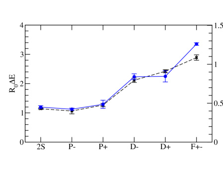
Figure 13: The energies of $Q\bar{q}$ states from Ref. [114]. The solid line uses dynamical fermions and the dashed line is a corresponding quenched calculation. The energies of the L-wave excited states and the S-wave radial excited state are relative to the ground state (1S) — see text for notation. These energies are given both in terms of GeV — right axis — and in the more usual Sommer units of $R_{0}\approx 0.5$ fm defined in Subsec. 1 — left axis.

A typical outcome is depicted in Fig. 13 from Ref. [114]. This is for a dynamical fermion calculation and a corresponding quenched calculation on a $16^{3}\times~{}24$ lattice. In both cases, for numerical reasons, the light quark has a mass that is approximately that of a strange quark. Since the heavy quark is static, the energies can be labelled by $L_{\pm}$, where the coupling of the light quark spin to the orbital angular momentum gives $j=L\pm 1/2$. The total angular momentum ($J$) is then obtained by coupling $j$ to the heavy quark spin giving $J=j\pm 1/2$. However, since the heavy quark spin interaction can be neglected, the latter two states are degenerate in energy i.e. the $P_{-}$ state will have $J^{P}=0^{+},1^{+}$ and the $P_{+}$ state will have $J^{P}=1^{+},2^{+}$ etc. The $D$-waves show the interesting feature that there appears to be little or no spin-orbit splitting between the $D_{-}$ and $D_{+}$ states — contrary to some expectations [115, 116] that there should be an inversion of the level ordering (with $L_{+}$ lighter than $L_{-}$) at larger $L$ or for radial excitations. This has important implications for phenomenological interpretations of the data. We return to this in Subsec. 3. For $F$-waves, only the energy from a spin independent mixed operator $F_{\pm}$ is shown. The latter is expected to approximately correspond to the usual spin-average of the $F_{-}$ and $F_{+}$ states.

9 Charge and Matter Distributions of Heavy-Light Mesons ($Q\bar{q}$)

In many cases, when phenomenological models are constructed to describe lattice data, the emphasis is on fitting the energies. However, there are other observables that can be measured on a lattice. Of potential value when constructing models are lattice data for radial distributions of various quantities such as the charge and matter densities, which can be measured using three-point correlation functions $C_{3}$. Here we concentrate on the radial distributions of the $\bar{q}$ in the $Q\bar{q}$ system, whereas in Ref. [117, 118] the much more ambitious task of measuring radial distributions in the $\pi,\ \rho,\ N$ and $\Delta$ is tackled. The reasons why distributions in few-quark systems have received much less attention are two-fold. Firstly, unlike energies, these distributions are not directly observable, but only arise in integrated forms such as sum rules, form factors, transition rates etc. Secondly, as will be seen later, their measurement on a lattice is more difficult and less accurate than the corresponding energies. In spite of this, it is of interest to extract lattice estimates of various spatial distributions.

1 Three-point correlation functions $C_{3}$

Figure 14: The two contributions to the three-point correlation function $C_{3}$.

When the light-quark field is probed by an operator $\Theta({\bf r})$ at $t=0$ as the heavy quark propagates from $t=-t_{2}$ to $t=t_{1}$, the result is the three-point correlation function depicted in Fig. 14. This involves two light-quark propagators — one ($G^{\prime}_{q}$) going from $t=-t_{2}$ to $t=0$ and a second ($G_{q}$) going from $t=0$ to $t=t_{1}$ and has the form

$$C_{3}(-t_{2},\ t_{1},\ {\bf r})=\\ \operatorname{Tr}\langle\Gamma^{\dagger}G_{Q}({\bf x},-t_{2};{\bf x},t_{1})\Gamma G_{q}({\bf x},t_{1};{\bf x+r},0)\ \Theta({\bf r})G^{\prime}_{q}({\bf x+r},0;{\bf x},-t_{2})\rangle,$$ (0.65)

which can be expressed in terms of the pseudofermion fields $\phi({\bf x},t)$ and $\psi({\bf x},t)$ — similar to that for $C_{2}$ in Eq. 4. Here the vertex $\Theta=\gamma_{4}$ for the charge (vector) distribution and 1 for the matter (scalar) density. Again the $\bar{Q}$-term in Fig. 14 ensures that $C_{3}$ is real, but now there are only two terms compared with the four for $C_{2}$ in Fig. 12. This is because the fields connected to the probe $\Theta$ must be local, since the purpose of the probe is to measure the charge or matter distribution at a definite point ${\bf r}$. Therefore, only those light quark propagators that involve the local basic field $\phi$ at ${\bf r}$ can be used, since the $\psi$ field contains contributions from $\phi$ fields at next-to-nearest neighbour sites and so is non-local. This must also be kept in mind when fuzzing is introduced to give a matrix $C_{3,ij}(-t_{2},\ t_{1},\ {\bf r})$. Here the fuzzing indices $i,j$ refer to the various fuzzing options of the $\psi$’s at the $Q\bar{q}$ vertices. As with the energies extracted from $C_{2}$, the fuzzing permits the measurement of excited state distributions.

2 Analysis of $C_{3}$

The analysis of the three-point correlation functions $C_{3}(\Theta,T=t_{1}+t_{2},{\bf r})$ is performed using a generalisation of the one for $C_{2}$ in Eq. 0.63, namely, fitting $C_{3,ij}(\Theta,T,{\bf r})$ with the parametric form

$$\tilde{C}_{3,ij}(\Theta,T,{\bf r})=\sum_{\alpha=1}^{M_{3}}\sum_{\beta=1}^{M_{3}}v_{i}^{\alpha}\exp[-m_{\alpha}t_{1}]x^{\alpha\beta}(r)\exp[-m_{\beta}(T-t_{1})]v_{j}^{\beta}.$$ (0.66)

The $m_{\alpha}$ and ${\bf v}$-vectors are those obtained by minimizing the $C_{2}$ in Eq. 0.63 and, for each value of $r$, the $x^{\alpha\beta}(r)$ are varied to ensure a good fit to $C_{3,ij}(\Theta,T,{\bf r})$ by the model expression $\tilde{C}_{3,ij}(\Theta,T,{\bf r})$.

Two forms of $x^{\alpha\beta}(r)$ have been used:

1. A non-separable (NS) form, where each $x^{\alpha\beta}(r)$ is treated as a single entity.

2. A separable (S) form $x^{\alpha\beta}(r)=y_{\alpha}(r)y_{\beta}(r)$. It is seen from Eq. 0.65 that this appears to be a more natural parametrization, since it contains the product of two light-quark propagators $G_{q}$. Also the $y_{\alpha}(r)$, to some extent, resemble a wave function for the state $\alpha$, since its square yields a distribution.

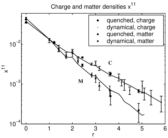
Figure 15: The ground state charge (C) and matter (M) densities [$x^{11}(r)$] as a function of $r/a$ from Ref. [59]. The lines shows a fit to these densities with a sum of two lattice exponential functions — see Subsec. 3. The scaled quenched results of Ref. [58] are also shown by filled circles and squares.

The outcome is shown in Fig. 15 for the ground state and in Fig. 16 for the excited states. Several points are of interest in Fig. 15:

• At small values of $r$ the two densities are comparable i.e. $x^{11}_{C}\approx x^{11}_{M}$.

• As $r$ increases from zero the matter density drops off faster than the charge density. A similar difference has also been seen in Ref. [118], where the authors measure these densities for the $\pi,\rho,N$ and $\Delta$ on a $16^{3}\times 32$ lattice with $\beta=6.0$ for both quenched and unquenched configurations.

• The densities calculated with the quenched approximation in
  Ref. [58] are the same, within error bars, as those for the full dynamical quark calculation of Ref. [59]. However, as will be discussed in Subsec. 4, the matter sum rule does seem to differ.

• The densities do not have a smooth variation with $r$, but, as will be shown in Subsec. 3, many of the kinks can be understood in terms of latticized forms of standard Yukawa, exponential or gaussian functions.

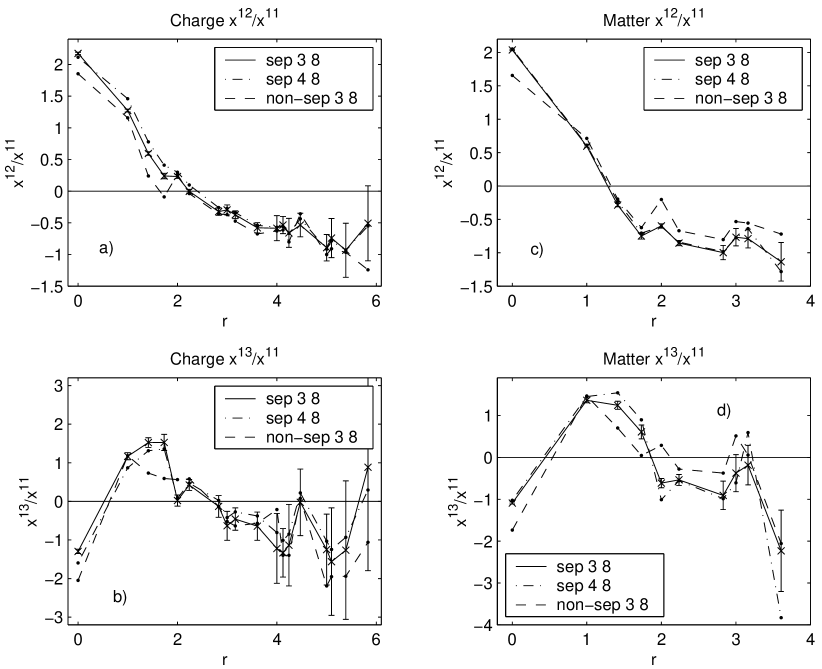
Figure 16: a) and b): The ratios $y_{2}(r)=x^{12}/x^{11}$ and $y_{3}(r)=x^{13}/x^{11}$ for the charge distribution. c) and d): These ratios for the matter distribution — see Ref. [59].

In Fig. 16 the excited state results are shown for different types of analysis. The label “sep” refers to the separable assumption for $x^{ij}$ and “non-sep” to the non-separable assumption. The two numbers associated with each set of data refer to $T_{2,{\rm min}}$ and $T_{3,{\rm min}}$ in Eq. 0.64 and the corresponding equation for Eq. 0.66. In this figure the main point of interest is the appearance of nodes. The presence of these nodes is very clear and also the number of nodes is as expected. The first excited state has a single node at about 0.3 fm in the charge case and about 0.2 fm for the matter. The second excited state seems to have two nodes with one being at about 0.1 fm and a second at about 0.4 fm for the charge and 0.3 fm for the matter. It will be a challenge for phenomenological models to explain these data.

When discussing the use of the separable form $x^{\alpha\beta}(r)=y_{\alpha}(r)y_{\beta}(r)$, it was stated that $y_{\alpha}(r)$ can possibly be interpreted as a wave function for the state $\alpha$. However, there are other radial distributions associated with the $Q\bar{q}$ system that can also be interpreted as wave functions. These are the Bethe–Salpeter wave functions $w_{\alpha}(r)$ discussed in Ref. [56]. They are extracted by assuming the hadronic operators $C_{\alpha\alpha}(r_{1},\ r_{2},\ T)$ to be of the form $w_{\alpha}(r_{1})w_{\alpha}(r_{2})\exp(-m_{\alpha}T)$, where the sink and source operators are of spatial size $r_{1}$ and $r_{2}$. Qualitatively, the forms of $y_{1}(r)$ and $y_{2}(r)$ plotted in Fig. 16 and the corresponding ones for $w_{1}(r)$ and $w_{2}(r)$ are found to be similar. However, even though they do bear some similarities, it should be added that there are several reasons why these two types of wave function should not agree in detail with each other. In particular, the $[w_{\alpha}(r)]^{2}$ cannot be identified as a charge or matter distribution. In addition, they are found by using an explicit fuzzed path between $Q$ and $\bar{q}$ and so are dependent on the fuzzing prescription, whereas the $y_{\alpha}(r)$ are defined in a path-independent way.

The above considers only S-wave distributions for both ground and excited states. The extension to other partial waves is now in progress [61]. Preliminary results for the $P_{-}$ state indicate that there the distributions are qualitatively of the form expected from a Dirac equation description i.e. the charge and matter distributions are not zero for $r=0$.

3 Fits to the radial forms

Fitting data with Yukawa, exponential and gaussian forms

In Figs. 15 and 16 the results are presented as a series of numbers. However, even though these are the actual lattice data, they are, in practice, not very convenient to use or interpret. To overcome this it is, therefore, useful to parametrize the data in some simple form. Furthermore the results in Fig. 15 do not follow smooth curves but exhibit several kinks. If the latter are first ignored, then average fits can be reasonably well achieved with simple Yukawa (Y), exponential (E) or gaussian (G) forms giving $\chi^{2}/n_{{\rm dof}}\approx 1.4$. The reason for using exponential and Yukawa radial functions is that they arise naturally as propagators in quantum field theory — usually in their momentum space form $(q^{2}+m^{2})^{-1}$, where $m$ can be interpreted as the mass of a meson being exchanged between the heavy quark and the point at which the light quark is probed. On the other hand, when going away from quantum field theory and attempting to understand the radial dependences in terms of wave functions from, for example, the Dirac equation, then gaussian forms can arise naturally — see Subsec. 3. However, this fitting can be greatly improved by using lattice versions (LY, LE, LG) of the above Yukawa, exponential or gaussian forms, namely

$$\left[\frac{\exp(-r/r^{{\rm LY}})}{r}\right]_{{\rm LY}}=\frac{\pi}{aL^{3}}\sum_{{\bf q}}\frac{\cos({\bf r}.{\bf q})}{D+0.25[a/r^{{\rm LY}}]^{2}},$$ (0.67)

$$\left[\exp(-r/r^{{\rm LE}})\right]_{{\rm LE}}=\frac{\pi a}{2r^{{\rm LE}}L^{3}}\sum_{{\bf q}}\frac{\cos({\bf r}.{\bf q})}{[D+0.25(a/r^{{\rm LE}})^{2}]^{2}},$$ (0.68)

$$\left[\exp[-(r/r^{{\rm LG}})^{2}]\right]_{{\rm LG}}=\left[\frac{r^{{\rm LG}}\sqrt{\pi}}{aL}\right]^{3}\sum_{{\bf q}}\cos({\bf r}.{\bf q})\exp[-(r^{{\rm LG}}/a)^{2}D].$$ (0.69)

Here $L$ is the lattice size along one axis and $D=\sum^{3}_{i=1}\sin^{2}(aq_{i}/2)$, where $aq_{i}=0,\ \frac{2\pi}{L},\ \ldots,\ \frac{2\pi(L-1)}{L}.$

These are able to give much of the kink structure in the data — as is seen in Fig. 17, where in each case two Yukawas, exponentials or gaussians are used to give the fits 2LY, 2LE and 2LG with $\chi^{2}/n_{{\rm dof}}\approx 1$. All three of these forms are equally acceptable [59].

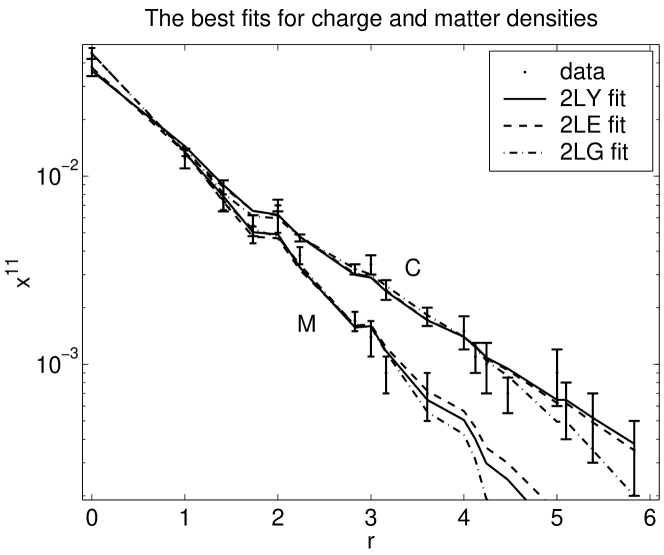
Figure 17: Fits to the lattice data in Fig. 15 with lattice exponential (2LE), Yukawa (2LY) and gaussian (2LG) forms from Ref. [59].

In the 2LE and 2LY fits it is of interest to express the range parameters $r^{{\rm LY}}$ and $r^{{\rm LE}}$ in terms of the mass ($1/r^{i}$) of the particle producing this range. Both types of fit find that the longest range corresponds to the exchange of a vector meson of mass $m^{v}_{0}\approx$1 GeV for the charge density and a scalar meson of mass $m^{s}_{0}\approx$1.5 GeV for the matter density. These masses of the mesons have been extracted in a rather indirect manner. However, in the literature there have been direct calculations of the energies of these $q\bar{q}$ states using the same lattice parameters and lattice size as those employed here. In Ref. [119] they got $m^{v}_{0}=1.11(1)$ GeV and in Ref. [120] $m^{s}_{0}=1.66(10)$ GeV — numbers consistent with the above indirect estimates.

It should be added that the expression LY in Eq. 0.67 is often used in the Coulomb limit $r^{{\rm LY}}\rightarrow\infty$ for discretizing the $1/r$ term of $V_{Q\bar{Q}}(r)$ in Eq. 0.6. However, in that limit the condition ${\bf q}\not=0$ is necessary.

Fitting $Q\bar{q}$ data with the Dirac equation

The above fits are purely phenomenological with there being no connection between the forms fitting the charge and matter distributions. However, there is an alternative approach in the spirit of an Effective Potential Theory (EPT), in which the data are fitted by the solutions of the Dirac equation. In the present situation using the Dirac equation and not the Schrödinger equation does not seem unreasonable on three counts:

1. The light-quark propagators are generated by a discretized form of the Dirac operator — see Subsec. 3.

2. The mass (or any effective mass) of the light quark is $\ll 1$ GeV, so that relativistic effects are expected.

3. Figs. 15 and 17 show that the charge and matter distributions are different — a feature not easy to understand in a non-relativistic Schrödinger approach, where the wave functions have only one component $\phi$, so that both the charge and matter distributions would be proportional to $|\phi|^{2}$. In comparison the Dirac equation has two components. Of course, one could also resort to the argument familiar in nuclear physics, when discussing the difference between the charge and matter RMS radii of nuclei, namely, that the matter distribution is the basic one with the charge distribution obtained by folding in the charge radius of an individual nucleon. We return to this in the next subsection.

In the notation that $G$ and $F$ are the large and small components of the solution to the Dirac equation then the charge ($C$) and matter ($M$) distributions can be expressed as

$$x_{C}^{\alpha\beta}(r)=G_{\alpha}(r)G_{\beta}(r)+F_{\alpha}(r)F_{\beta}(r)\ \ {\rm and}\ \ x_{M}^{\alpha\beta}(r)=G_{\alpha}(r)G_{\beta}(r)-F_{\alpha}(r)F_{\beta}(r)$$

respectively. Attempts are now underway [57] to study to what extent the above distributions can indeed be interpreted by these two relationships.

Since we are now in the realm of EPTs, we need the three ingredients discussed in Subsec. 2 — a wave equation (now the Dirac equation), a potential $V_{Q\bar{q}}$ and an effective quark mass (a free parameter). The main problem is the form of $V_{Q\bar{q}}$, since it is not at all clear whether the “natural” generalisation of the form appropriate for static quarks in Eq. 0.6 to

$$V_{Q\bar{q}}(r)=-\frac{e}{r}+b_{s}r\gamma_{4},$$ (0.70)

is correct. Here the first term is treated as a four-vector simply by the analogy between one-gluon exchange and one-photon exchange. However, if this term for large $r$ is in fact the so-called Lüscher term [122], a vibrating string correction of $-\pi/(12r)$ to the leading string term $b_{s}r$, then it should be a scalar. On the other hand, there are theoretical reasons that partially justify the use of the Dirac equation for heavy-light mesons with the form for the potential in Eq. 0.70. For example, in Ref. [121] the authors derive a Dirac equation for a heavy-light meson by starting from the QCD Lagrangian and taking into account both perturbative and nonperturbative effects. The Coulomb-like effect is treated rigorously and the confining potential heuristically. The outcome is that the confining potential is a scalar and the Coulomb part is the fourth component of a 4-vector. However, the lack of any significant $D$-wave spin-orbit splitting, as is seen in Fig. 13, does suggest that the confining potential can not be purely scalar. This follows from the simple argument that, in a heavy(static)-light quark system, a central potential of the form $V(r)=a/r+br$ should give rise to a spin-orbit potential

$$V_{SO}(r)=-\frac{1}{4m^{2}r}\frac{dV}{dr}=\frac{1}{4m^{2}}(\frac{a}{r^{3}}-\frac{b}{r}).$$ (0.71)

Such a potential would lead to inversion of the level ordering (with $L_{+}$ lighter than $L_{-}$) at larger $L$ or for radial excitations and this is not seen in Fig. 13. The authors of Ref. [32], in fact, give arguments why the interquark confining potential should have the form

$$V(r)=a/r+br{(1+\gamma_{4})}/2$$ (0.72)

leading to simply

$$V_{SO}(r)=\frac{1}{4m^{2}}\frac{a}{r^{3}},$$ (0.73)

which would rapidly vanish at larger $L$. In Ref. [123] the electromagnetic structure functions of a heavy(static)-light quark system interacting via the potential in Eq. 0.72 are calculated. This ambiguity between the vector vs scalar structure of $V_{Q\bar{q}}$ is an ongoing argument — see Ref. [32] for a list of references on this controversy. Also, as mentioned in Subsec. 2, form factor effects reduce the rôle of any one-gluon exchange and that this loss of vector-like attraction could be replaced by a very short ranged instanton–generated scalar interaction.

An interesting property of the solutions to the Dirac equation is that, for a linearly rising potential, both the large $(G)$ and small $(F)$ components decay asymptotically as gaussians. This follows from the observation that the coupled Dirac equations for large $r$ can be written as

$$-m(r)G(r)=-F^{\prime}(r)\ \ {\rm and}\ \ m(r)F(r)=G^{\prime}(r),$$ (0.74)

where $m(r)=m+cr\rightarrow cr$ as $r\rightarrow\infty$ giving asymptotically the simple harmonic oscillator equation $G^{\prime\prime}+(cr)^{2}G=0$. This was the reason for considering not only Yukawa and exponential but also gaussian forms in the last subsection.

Fitting $Q\bar{q}$ data with the Schrödinger equation

In the previous subsection three reasons were given for attempting to fit the lattice data with the Dirac equation. However, two of these reasons are far from compelling — only the fact that the effective light-quark mass being $\ll 1$ GeV seems unavoidable. The comparison with the discretized Dirac operator used in the lattice simulation, as mentioned in Subsec. 3, is nothing more than an analogy without theoretical basis. Secondly, the fact that the charge distribution has a longer range than that for the matter is reminiscent of the difference between the charge and matter radii of nuclei. There this is usually expressed as

$$\langle r^{2}\rangle_{\rm charge}=\langle r^{2}\rangle_{\rm matter}+\langle r^{2}\rangle_{\rm proton},$$ (0.75)

relating the Mean Square Radius of the nuclear charge distribution with that for the matter distribution and the proton charge radius. This suggests that there is only one basic distribution — that of the matter — with the charge distribution arising from a finite size correction to the charge of the light-quark. This should not be surprising since the effective quark mass $(m_{q,\ {\rm effective}})$ is quite different (larger) compared with that used in the lattice calculation, which is about that of the strange quark. Here we are now saying that, in addition to a mass renormalisation, the light-quark develops a charge form factor. A direct application of Eq. 0.75 on the fits to the data in Fig. 17 results in $\bar{q}$ RMS charge radii of 0.51(4), 0.49(7) and 0.35(3) fm for the Yukawa, exponential and gaussian fits respectively. These are sizes consistent with $m_{q,\ {\rm effective}}\sim 500$ MeV (i.e. $1/m_{q,\ {\rm effective}}\approx 0.4$ fm) and are surprisingly large being 2-4 lattice spacings. Also $\bar{q}$ charge form factors of this size qualitatively explain why in Fig. 16 the node in the $x^{12}/x^{11}$ charge distribution is at a larger value of $r$ than that for the matter.

Since the problem has been reduced to only one basic distribution, we are now able to use an Effective Potential Theory (EPT) based on a non-relativistic Schrödinger equation. As before, the other two ingredients for an EPT are $m_{q,\ {\rm effective}}$ (a free parameter) and the potential $V_{Q\bar{q}}$ presumably based on the form appropriate for static quarks in Eq. 0.6.

In Ref. [60], when analysing the $Q^{2}\bar{q}^{2}$ lattice data of Ref. [77], this strategy was used first to extract a value of $m_{q,\ {\rm effective}}$ by fitting the spin-averaged energies of the $Q\bar{q}$ system — see Fig. 18.

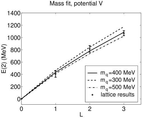
Figure 18: Fits to the spin-averaged energies in Fig. 13 for a series of values for $m_{q}$.

The outcome was $m_{q,\ {\rm effective}}\approx 400$ MeV — a value consistent with the above size estimate. We return to this in Subsec. 2. The above approach has also been carried out in Ref. [117], where nucleon charge correlations are measured and then fitted with a non-relativistic Schrödinger equation. First the authors extract two entities $C(r_{\Delta})$ and $C(r_{Y})$, which they interpret as the nucleon wave functions in either the coordinate $r_{\Delta}=(r_{12}+r_{23}+r_{13})$ — the so-called $\Delta$-Ansatz — or the coordinate $r_{Y}={\rm Min}(r_{1\epsilon}+r_{2\epsilon}+r_{3\epsilon})$, where ${\bf\epsilon}$ is the junction at which the three flux tubes meet. They then go on to fit this data with Airy functions that decay as $\exp(-cr^{3/2})$. These are the wave functions expected from a non-relativistic Schrödinger equation when using linearly rising potentials $V(r_{\Delta})\propto r_{\Delta}$ or $V(r_{Y})\propto r_{Y}$. In this way, fitting the $C(r_{\Delta},r_{Y})$ data seemed to slightly favour the $\Delta$-Ansatz. However, it should be added that this conclusion is far from being universally accepted. For example, in Ref. [124] the authors say:“In particular the $\Delta$-shape configuration debated in the literature is shown to be impossible and the well-known Y-shaped baryon is the only possibility.” This latter result is supported in Refs. [125, 126].

Fitting $Q\bar{q}$ data with semirelativistic equations

The equations considered in the above subsections are two extremes with the Dirac equation being fully relativistic and the Schrödinger equation completely non-relativistic. However, if — as in the “real” $B$-meson — the heavy quark is not static, then other possibilities arise when the basic Bethe–Salpeter equation is reduced in a systematic way to a Lippmann–Schwinger form. As mentioned in Subsec. 2 this can be carried out in a variety of ways, which give rise to the Blankenbecler–Sugar, Gross, Kadyshevsky, Thompson, Erkelenz–Holinde and other equations [35]. Unfortunately, these equations are not so easy to treat because of the unavoidable presence of the typical relativistic factors $\sqrt{m_{i}/E_{i}}$, where $E_{i}=\sqrt{m_{i}^{2}+{\bf p_{i}}^{2}}$ is the energy of a single particle of momentum ${\bf p_{i}}$. This automatically leads to a non-local interaction in coordinate space, since a local interaction requires a function of the relative momentum ${\bf q}={\bf p_{a}}-{\bf p_{b}}$. When dealing with one-gluon exchange this does not present a problem, since there the basic interaction is $\propto 1/q^{2}$ and so the equations can be formulated directly in momentum space. However, as seen in Eq. 0.6, a crucial part of the interquark interaction is the confining term $b_{s}r$ — an interaction that can not be conveniently treated directly in momentum space. In the literature there are several attempts to fit directly the meagre experimental $B$-meson data with these forms. For example, in Refs. [126] and [127] the Gross and Blankenbecler–Sugar equations, respectively, are employed to interpret the $B$-meson spectrum and a series of available transition rates.

Some of the complications that arise when dealing with the above equations can be partially overcome by using instantaneous interactions. Shortly after formulating the Bethe-Salpeter (B-S) equation in 1951 [128], Salpeter in 1952 [129] replaced the interaction $G(q^{2}={\bf q}^{2}-q_{4}^{2})$ in the B-S equation by its three dimensional counterpart $G({\bf q}^{2})$. This resulted in an equation for two particles $a$ and $b$, which could be written in the centre–of–mass system as

$$[E-H_{a}({\bf p})-H_{b}({\bf p})]\phi({\bf p})=P\int d^{3}q\gamma_{4}^{a}G({\bf q})\gamma_{4}^{b}\phi({\bf p}+{\bf q}),$$ (0.76)

where $H_{i}({\bf p})=m_{i}\beta^{i}+\bm{p.\alpha^{i}}$ with $\beta$ and $\bm{\alpha^{i}}$ being the usual Dirac matrices. The operator $P=\Lambda^{a}_{+}\Lambda^{b}_{+}-\Lambda^{a}_{-}\Lambda^{b}_{-}$ is a combination of the projection operators $\Lambda^{a}_{\pm}=[E_{a}(p)\pm H_{a}({\bf p})]/E_{a}(p)$, where $E_{a}(p)=\sqrt{m_{a}^{2}+{\bf p}^{2}}$. It should be added that Eq. 0.76 differs from an earlier one by Breit in 1929 [130] by the presence of the $P$ factor. In the nonrelativistic limit both equations reduce to the same form, but in general the Breit equation has a more limited applicability than Eq. 0.76 — as discussed in Ref. [129].

In Refs. [131], Eq. 0.76 is further simplified by first considering only positive-energy solutions i.e. omit the $\Lambda^{a}_{-}\Lambda^{b}_{-}$ terms in $P$. This results in the reduced Salpeter equation

$$[E-\sqrt{m_{a}^{2}+{\bf p}^{2}}-\sqrt{m_{\smash[t]{b}}^{2}+{\bf p}^{2}}\ ]\phi({\bf p})=\int d^{3}q\Lambda^{a}_{+}\gamma_{4}^{a}G({\bf q})\gamma_{4}^{b}\Lambda^{b}_{+}\phi({\bf p}+{\bf q}).$$ (0.77)

Then the formalism is further restricted to the positive energy components to give the semirelativistic spinless–Salpeter equation

$$[\sqrt{m_{a}^{2}+{\bf p}^{2}}+\sqrt{m_{\smash[t]{b}}^{2}+{\bf p}^{2}}+V(x)]\psi=E\psi,$$ (0.78)

where $V(x)$ is the Fourier transform of the $G({\bf q})$. Finally the authors of Refs. [131] go one more step by studying the equal mass case

$$[\beta\sqrt{m^{2}+{\bf p}^{2}}+V(x)]\psi=E\psi,$$ (0.79)

where, instead of fixing $\beta$ at 2, they show that $\beta>0$ can simulate the effect of several particles all of mass $m$. They interpret this equation as “the generalization of the nonrelativistic Schrödinger Hamiltonian towards relativistic kinematics” and study algebraically its properties for a variety of forms for $V(x)$. The reason why these authors go through explicitly the simplification of Eq. 0.76 is to show that Eq. 0.79 — the obvious extension of the Schrödinger equation — can indeed be derived in a systematic manner and is not just an educated guess.

4 Sum rules

In addition to measuring $C_{3}({\bf r})$ for various values of ${\bf r}$, the correlation where ${\bf r}$ is summed over the whole lattice is also obtained. This leads to the charge sum rule as discussed in Ref. [59]. For the charge distribution, the outcome is that $\sum_{\bf r}x^{11}({\bf r})=X^{11}$ is $\approx 1.3(1)$, which is consistent with the earlier quenched result [58]. The fact that $X^{11}$ is not unity, as expected in the continuum limit, can be qualitatively understood by introducing a renormalisation factor of $\approx 1/1.3\approx 0.8$ into the basic $\gamma_{4}$ vertex used to measure the charge density. Such a factor of this magnitude is reasonable as shown in Ref. [132]. It is also reassuring that the $X^{\alpha\beta}$ with $\alpha\not=\beta$ are, in general, consistent with zero — as expected in the continuum limit.

The matter sum rule has a somewhat wider spread of values with 0.9(1) being a reasonable compromise — a number that is about twice the estimate of 0.4(1) for the quenched calculation of Ref. [58]. Perhaps this is an indication that, unlike the corresponding matter radial distributions in Figure 15, the quenched and unquenched results, due to the effect of disconnected processes, can differ even with the present sea–quark masses of about that of the strange quark. Certainly differences should appear with very light sea–quarks, since then the contribution from the disconnected processes, that only enter for the matter distributions, can become significant. However, we do not have the data to cross check with Refs. [74], which advocate the existence of such differences for the matter sum rule.

The fact that the matter sum rule is considerably less than that for charge can be qualitatively understood by employing data from different hopping parameters ($\kappa$) and using the identity

$$X^{11}=\frac{d(am_{1})}{d\kappa^{-1}},$$ (0.80)

where $am_{1}$ is the ground state energy and $\kappa$ the hopping parameter — see Subsec. 2 and Ref. [74]. When the $m_{1}$’s correspond to the cases where the light quark is of about one and two strange quark masses, Refs. [74] and  [56] give $X^{11}\approx$ 0.34(8) and 0.31(6) respectively — consistent with the present value of 0.4(1). These values are also consistent with the following simple estimate: If the $Q\bar{q}$-meson mass $(am_{1})$ is taken to be simply the sum of the quark masses i.e. $am_{Q}+am_{q}$ and $\kappa^{-1}=8+2am_{q}$, then Eq. 0.80 gives

$$X^{11}=\frac{d(am_{Q}+am_{q})}{d(8+2am_{q})}=0.5.$$ (0.81)

Another reason for expecting $X^{11}_{M}<X^{11}_{C}$ also follows from a potential approach using the Dirac equation as in Subsec. 3. This results in $X^{11}_{C}\sim G_{1}^{2}+F_{1}^{2}$ and $X^{11}_{M}\sim G_{1}^{2}-F_{1}^{2}$. Here $G_{1}^{2}$ and $F_{1}^{2}$ are integrals of the large and small components of the solution to the Dirac equation.

10 The $B-B$ System as a $[(Q\bar{q})(Q\bar{q})]$ Configuration.

In Secs. 8 and 9 the energies and some radial distributions of a single heavy-light meson were studied. In this section the interaction between two such mesons is extracted using lattice QCD and the outcome is fitted with an extension of the $f$-model developed earlier for the $[(Q\bar{Q})(Q\bar{Q})]$ system in Secs. 5 and 7. However, it should be added that the study of $[(Q\bar{q})(Q\bar{q})]$ configurations is much less academic than their $[(Q\bar{Q})(Q\bar{Q})]$ counterparts. Many years ago simple multi-quark systems have been proposed to exist as bound states [133, 134, 135]. Also four quarks forming colour singlets or as bound states of two mesons are candidates for particles lying close to meson–antimeson thresholds, such as $a_{0}(980),\ f_{0}(980)$ ($K\bar{K}$), $f_{0}(1500),\ f_{2}(1500)$ ($\omega\omega,\ \rho\rho$), $f_{J}(1710)$ ($K^{*}\bar{K}^{*}$), $\psi(4040)$ ($D^{*}\bar{D}^{*}$), $\Upsilon(10580)$ ($B^{*}\bar{B}^{*}$) [111]. Systems involving $b$ quarks are particularly interesting since they should be more easily bound provided the potential is attractive, since the repulsive kinetic energy of the quarks is smaller, while the attractive two-body potential remains the same. In so-called deuson models [136] the long-range potential between two mesons comes from one-pion exchange, suggesting that meson–meson systems are significantly less bound than meson–antimeson systems. Other models used for realistic four-quark systems include string-flip potential models (see Ref. [138] for a review), bag models [134], and a model-independent approach [139]. In fact four-quark states with two heavy quarks have been predicted to be stable [140]. Most models give stability for systems where the heavy quarks have the $b$ mass, but long range forces might push the required heavy-to-light mass ratio down sufficiently so that $cc\bar{q}\bar{q}$ states would be bound as well.

1 Lattice calculation of the $[(Q\bar{q})(Q\bar{q})]$ system

The interaction between two $(Q\bar{q})$ states is depicted in Fig. 19 as a sum of two terms — the uncrossed and crossed diagrams. In the latter diagram the $\bar{q}$ hops from one $Q$ to the other.

Figure 19: The interaction between two $(Q\bar{q})$ states — the so-called uncrossed and crossed diagrams. The solid lines represent $Q$’s and the wavy ones $\bar{q}$’s.
NB Compared with earlier figures such as Figs. 12 and 14 the Euclidean time direction is now horizontal.

Exploratory studies of two-meson systems have been made for the cross diagram only for SU(3) colour [141] and for both diagrams in Refs. [142], [143] for SU(2), SU(3) colour respectively. This topic is also discussed in Sec. 2.4 of Chapter 2 and Subsec. 4.4.3 of Chapter 4.

In Refs. [77, 144] quenched lattices are used with SU(3) colour and static heavy quarks with light quarks of approximately the strange quark mass. Also, when the two $Q$’s are at the same point (i.e. $R=0$) and by using the SU(3) colour relationship $3\otimes 3=\bar{3}\oplus 6$, then the two $Q$’s behave like a $\bar{Q}$. This equivalence implies that the $I_{q}=1,\ S_{q}=1$ state will have the same light quark structure as the $\Sigma_{b}$ baryon and the $I_{q}=0,\ S_{q}=0$ state as that of the $\Lambda_{b}$ baryon. The other two allowed states at $R=0$ correspond to a static sextet source. When the results for $R=0$ are compared with the known spectrum of baryons with one heavy quark ($\Lambda_{b}$ and $\Sigma_{b}$), good agreement is found. Note that this link to baryons at small separation $R$ cannot be explored using SU(2) of colour.

Below, the mass of one quark in each meson is taken to be very heavy — the prototype being the $B$-meson. The static limit is then the leading term in the heavy quark effective theory for a heavy quark of zero velocity and there will be corrections of higher orders in $1/m_{Q}$, where $m_{Q}$ is the heavy quark mass. In the limit of a static heavy quark, the heavy quark spin is uncoupled since the relevant magnetic moment vanishes which implies that the pseudoscalar $B$-meson and the vector $B^{*}$-meson will be degenerate. This is a reasonable approximation since they are split by only 46 MeV experimentally, which is less than 1% of the mass of the mesons — see Table 3. Since it is often convenient to treat these two mesonic states as if they were degenerate, here they are described collectively as the ${\cal B}$-meson. Because of the insensitivity to the heavy quark spin, it is then appropriate to classify these degenerate ${\cal B}$-meson states by the light quark spin. The system of two heavy-light mesons at spatial separation $R$ will be referred to as the ${\cal BB}$ system. With both heavy-light mesons static, this ${\cal BB}$ system is then described by the two independent spin states of the two light quarks in the two mesons i.e. $S_{q}=0$ and 1. Thus there are four possible states and it is necessary to classify the interaction in terms of these spin states.

This situation is very similar to that of the hydrogen molecule in the Born–Oppenheimer approximation — with, however, the additional possibility that the two “electrons” can have different properties. Another similarity is with the potential between quarks which has a central component and also scalar and tensor spin-dependent contributions.

Each ${\cal B}$-meson will have a light quark flavour assignment. For the ${\cal BB}$ system, it will be appropriate to classify these states according to their symmetry under interchange of the light quark flavours. For identical flavours (e.g. ${s}s$ or ${u}u$), we have symmetry under interchange, whereas for non-identical flavours (e.g. ${s}u$ or ${d}u$), we may have either symmetry or antisymmetry. For two light quarks, it is convenient to classify the states according to isospin as $I_{q}=1$ (with $uu$, $ud+du$ and $dd$) or $I_{q}=0$ (with $ud-du$). To ensure overall symmetry of the wave function under interchange and, assuming symmetry for spatial interchange, the flavour, total light quark spin ($S_{q}$) and total heavy quark spin ($S_{b}$) must be combined to achieve this. Thus in the limit of an isotropic spatial wave function i.e. $L=0$, there will be four different ground state levels of the ${\cal BB}$ system labelled by $(I_{q},\ S_{q})$ in the following discussion. These are shown in Table 4.2 of Chapter 4.

To check for possible finite size effects, the numerical analysis was carried out on quenched lattices of sizes $12^{3}\times 24$ and $16^{3}\times 24$, at $\beta=5.7$, corresponding to $a\approx 0.18$ fm. The bare mass of the light quark was near that of the strange mass and light quark propagators were generated using the Maximal Variance Reduction method in Subsec. 3. This enabled measurements of the strength of the interaction to be made out to separations of $R\approx 8$, which corresponds roughly to 1.4 fm.

As seen in Figs. 2.5, 2.6 of Chapter 2 and Figs. 4.21 of Chapter 4, attraction between two ${\cal B}$ mesons is found at small values of $R$ for $(I_{q},S_{q})$=(0,0) and (1,1) and at moderate $R$ ($\sim$0.5 fm) for (1,0) and (0,1). For very heavy quarks, this will imply binding of the ${\cal BB}$ molecules with these quantum numbers and $L=0$ — see Sec. 2.4 of Chapter 2 for more details.

It is also possible to extract from the lattice data quantities that can be identified as $\pi$- and $\rho$-exchange between the two ${\cal B}$-mesons. This is shown in Fig. 20.

Figure 20: The ratio of the crossed-diagram contributions to the spin-averaged uncrossed contribution to the ${\cal BB}$ correlation. The meson exchange expressions, $\exp(-MR)/R$, are compared with these results — using pion exchange with $M=580$ MeV (continuous line) and rho exchange with $M=890$ MeV (dash-dotted line). Note that the pion exchange expression is normalised as described in the text, whereas the rho exchange contribution has an ad hoc normalisation. Here $R$ is in units of $a\approx 0.18$ fm [77].

For the $\pi$-exchange at large $R$ the potential is expected to be of the form

$$V(R)=\vec{\tau}_{1}.\vec{\tau}_{2}\frac{g^{2}M^{2}}{4\pi f_{\pi}^{2}}\frac{e^{-MR}}{R},$$ (0.82)

where $g/f_{\pi}$ is the pion coupling to quarks [136]. From the lattice studies of $BB^{*}\pi$ coupling  [145] the value of $g=0.42(8)$ is predicted and $f_{\pi}$ is the pion decay constant (132 MeV). Because the comparison with the lattice results is for light quarks, the pion mass is taken to be $Ma=0.53$ i.e. a “pion” of mass $\approx 580$ MeV — a value appropriate for this lattice. Therefore, in Fig. 20 the solid curve being compared with that data containing one-pion-exchange is from Eq. 0.82 and is seen to have the correct features — giving support, at these large values of $R$, for the deuson model of Ref. [136]. However, the corresponding $\rho$-exchange comparison with the dash-dotted line in Fig. 20 is less informative, since the normalisation is ad hoc.

Even though the agreement with one-pion-exchange is seen to be very good, the authors of Ref. [77] are quick to point out that their result is “better than should be expected” and give arguments why “This implies that we should not take our estimate of the magnitude of one pion exchange as more than a rough guide at the $R$-values we are able to measure.” It is possible that here we are seeing an effect reminiscent of the Chiral Bag Model described by Myhrer in Chapter 4 of Ref. [36]. In such models there are pion fields outside some radius $r_{b}\approx 0.5$ fm and only quarks inside $r_{b}$. Calculations of one-pion-exchange potentials (OPEP) between, say, two nucleons then naturally give the usual form of OPEP for $r>r_{b}$. However, for some smaller values of $r$ the interaction seems to be simply a continuation of this “usual form of OPEP” i.e. there is a precocious onset of OPEP in a region where there are no pions. Perhaps it is this that is being seen in Ref. [77] and Fig. 20. It should be added that in some studies of interacting clusters, the OPEP is expected to emerge with an exponential dependence and not the Yukawa form in Eq. 0.82. This has been demonstrated in Ref. [71], where the authors show that this unconventional form of OPEP is due to the use of the quenched approximation. To avoid this problem with the long range part of the interaction, in a later paper [137] these authors study the $\Lambda_{Q}\Lambda_{Q}$ potential, which does not contain a one-pion or one-eta contribution.

2 Extension of the $f$-model to the $[(Q\bar{q})(Q\bar{q})]$ system

In Sec. 5 a model was developed for understanding the lattice energies of four static quarks $Q({\bf r_{1}})Q({\bf r_{2}})\bar{Q}({\bf r_{3}})\bar{Q}({\bf r_{4}})$ in terms of two-quark potentials and is summarised by Eqs. 0.37, 0.38. This f-model, although very simple, contains the same basic assumptions made in the more elaborate many-body models that incorporate kinetic energy e.g. the Resonating Group Method described by Oka and Yazaki in Chapter 6 of Ref. [36]. It is, therefore, reasonable that this simplified f-model can to some extent check the validity of these more elaborate counterparts. In Ref. [60] the model in Sec. 5 was extended as below to study the interaction between two $Q\bar{q}$ mesons. This resulted in a non-relativistic Schrödinger-like equation

$$|{\bf K}^{\prime}(R)+{\bf V}^{\prime}(R)-E(4,R){\bf N}^{\prime}(R)|\psi=0$$ (0.83)

— for more details see Appendix B.

So far this model has only been developed for spin independent potentials, which means that it should only be compared with the spin-averaged results of Ref. [77] shown in Fig. 4.21 in Chapter 4. The outcome from Refs. [60, 146] is shown in Fig. 21, where it is seen by the solid line that the use of only two-quark potentials (i.e. in the weak coupling limit $f=1$ or $k_{f}=0$) results in a considerable overbinding at $R=0.18$ fm. The dashed line shows the effect of using a form factor with $k_{f}=0.6$.

Figure 21: Comparison between the spin independent part of the $Q^{2}\bar{q}^{2}$ binding energies calculated on a lattice [77] (solid circles – quenched approximation with $a=0.170$ fm) [147] (solid squares – with dynamical fermions and $a=0.142$ fm). The crosses, with the solid line to guide the eye, show the model in the weak coupling limit ($k_{f}=0$). The dotted line shows the result with $k_{f}$ =0.6 and $m_{q}$=400 MeV. The dynamical fermion data was not used in any fit. They are simply included to show that it is qualitatively consistent with the quenched data but with considerably smaller error bars.

Admittedly this is less convincing than the earlier four static quark case, since the conclusion depends essentially on only the two data points corresponding to the two $Q$’s being 1 and 2 lattice spacings apart. However, the fact that $k_{f}$ is consistent with $\bar{k}\approx 0.5(1)$ — see Fig. 8 — the corresponding parameter needed in Subsec. 5 for $[(Q\bar{Q})(Q\bar{Q})]$ configurations in squares or near-squares lends support to the general approach of this model.

In Refs. [148] $BB$-scattering has been treated in the weak coupling limit of $k_{f}=0$ — a limit that appears to be ruled out by the comparison in Fig. 21. However, it is possible that this limit can, to some extent, be salvaged if the model is extended by including states with excited glue — as in Sec. 7 and Appendix A.3 for the $[(Q\bar{Q})(Q\bar{Q})]$ system.

11 The $B-\bar{B}$ System as a $[(Q\bar{q})(\bar{Q}q)]$ Configuration

The $B$-factories discussed in Subsec. 1 are not able to study directly $BB$ reactions. However, the related $B\bar{B}$ system is accessible as a final state in the decay of the $\Upsilon(4S,10580\ {\rm MeV})$, whose main branching ($\geq 96\%$) is into $B\bar{B}$.

At first sight it may be thought that the $[(Q\bar{q})(\bar{Q}q)]$ and $[(Q\bar{q})(Q\bar{q})]$ configurations have similar properties. However, this is not so, since now the $q$ and $\bar{q}$ can annihilate each other. This means that there is a coupling between $(Q\bar{Q})$ and $[(Q\bar{q})(\bar{Q}q)]$ states i.e. the string (flux) connecting the $Q$ and $\bar{Q}$ in the $(Q\bar{Q})$ state can break into two mesons $(Q\bar{q})$ and $(\bar{Q}q)$. This becomes very clear if the mechanism for the interaction between two $(Q\bar{q})$ states, shown in the Fig. 19, is compared with the corresponding ones for the present $[(Q\bar{q})(\bar{Q}q)]$ case on the first row of Fig. 22 — only the uncrossed contributions look similar.

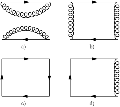
Figure 22: The $[(Q\bar{q})(\bar{Q}q)]$ interaction and string breaking.
The a) uncrossed and b) crossed $[(Q\bar{q})(\bar{Q}q)]\rightarrow[(Q\bar{q})(\bar{Q}q)]$ contributions to the interaction; c) The $(Q\bar{Q})\rightarrow(Q\bar{Q})$ Wilson loop and d) the $[(Q\bar{q})(\bar{Q}q)]\rightarrow(Q\bar{Q})$ off-diagonal correlation.

The diagram b) represents the two step process involving the annihilation and creation of a $q\bar{q}$ pair

$[(Q\bar{q})(\bar{Q}q)]{\bf\longrightarrow}(Q\bar{Q}){\bf\longrightarrow}[(Q\bar{q})(\bar{Q}q)].$

This breaking of a long flux tube between two static quarks into a quark–antiquark pair is one of the most fundamental phenomena in QCD. Because of its highly non-perturbative nature it has defied analytical calculation, while its large scale, e.g. when compared to the sizes of composite particles in the theory, has caused difficulties in standard nonperturbative methods. Thus string breaking has remained a widely publicized feature of the strong interaction that has never, apart from rough models, been reproduced from the theory.

String breaking can occur in hadronic decays of $Q\bar{Q}$ mesons and is especially relevant when this meson is lying close to a meson–antimeson ($Q\bar{q})(\bar{Q}q$) threshold. Its effect should be seen most directly by measuring the $Q\bar{Q}$ potential, since the onset of string breaking would change the form of the standard $Q\bar{Q}$ potential in Eq. 0.6 so that the confining term — $br$ for all $r$ — would become $br$ only for $r<r_{c}$ and have the constant value $br_{c}$ for $r>r_{c}$. Unfortunately, this direct approach of trying to see the flattening in the static $Q\bar{Q}$ potential at large separation has only had limited success. An example[149] of the usual outcome is seen in Fig. 23. There the potential $V(Q\bar{Q})$ continues to rise linearly way past the value of $r/r_{0}\approx 2.4$, where the breaking into two mesons should occur — denoted by the horizontal dotted lines. There is clearly no sign of the expected flattening.

Figure 23: The static potential $V(Q\bar{Q})$ obtained from simply the Wilson loop of Fig. 1. N.B. There is no sign of the expected flattening at $r/r_{0}\approx 2.4$, where it becomes energetically favourable to create two mesons[149].

The failure of this Wilson loop method seems to be mainly due to the poor overlap of the operator(s) with the $[(Q\bar{q})(\bar{Q}q)]$ state [150, 151]. In three-dimensional SU(2) with staggered fermions an improved action approach has been claimed to be successful with just Wilson loops [152]. However, in full QCD with fermions, effective operators for $[(Q\bar{q})(\bar{Q}q)]$ systems are hard to implement; part of the problem is the exhausting computational effort required to get sufficient statistics for light quark propagators with conventional techniques for fermion matrix inversion. In Ref. [153] this problem was to a large extent overcome by applying the Maximal Variance Reduction method of Subsec. 3 using SU(3) on a $16^{3}\times 24$ lattice with the Wilson gauge action plus the Sheikholeslami–Wohlert quark action and $\beta=5.2$ (i.e. $a\approx 0.14$ fm) with two degenerate flavours of both valence– and sea–quarks.

Since Fig. 22 b) is a two-step process it is natural to consider the process as a coupled channels problem between the $[(Q\bar{q})(\bar{Q}q)]$ and $(Q\bar{Q})$ configurations. This leads to the two new processes in Fig. 22 d) and c) — the off-diagonal term $[(Q\bar{q})(\bar{Q}q)]{\bf\longleftrightarrow}(Q\bar{Q})$ and the corresponding diagonal term $(Q\bar{Q}){\bf\longleftrightarrow}(Q\bar{Q})$, which is nothing more than the Wilson loop discussed in Subsec. 1.

In Fig. 24 the results from a calculation using just the most fuzzed basis states for both $(Q\bar{Q})$ and $[(Q\bar{q})(\bar{Q}q)]$ (a $2\times 2$ matrix) are shown. Unfortunately, the statistics are not sufficient to give accurate plateaux for the energies. However, the authors of Ref. [153] are able to extract a quantity they call the mixing matrix element $x$, which can be interpreted as an indirect measure of possible string breaking. They find that $x=48(6)$ MeV. At $r_{c}$ one would expect the ground and excited state energies to be separated by $2x$. However, in Fig. 24 a larger separation is observed, which is presumably again due to insufficient statistics.

Figure 24: Ground and excited state from a variational calculation including $Q\bar{Q}$ and $Q\bar{q}\bar{Q}q$ operators [153]. The highest fuzzed basis state for both is used here. The ground state of the Wilson loop and $2m_{Q\bar{q}}$ are also shown.

In Ref. [154], utilizing the SU(3) colour relationship $3\otimes\bar{3}=1\oplus 8$, the $Q\bar{Q}$ at $R=0$ behave as a singlet(vacuum), so that the remanent $q\bar{q}$ component with $(S_{q\bar{q}},I_{q\bar{q}})=(0,1)$ can be compared successfully to a pion with non-zero momentum.

In the above, the failure of the $Q\bar{Q}$ correlations alone to give a flattening of $V(Q\bar{Q})$ was considered a negative feature. However, in the Conclusion it will be seen that this “failure” could be useful for constructing models.

So far no one has attempted to understand this $B\bar{B}$ data with the extended $f$-model of Subsec. 2 for $BB$ states. Such an extension would also have to incorporate $q\bar{q}$ creation and annihilation using some model such as the so-called Quark Pair Creation or ${}^{3}P_{0}$ model [155]. When this ${}^{3}P_{0}$ model was combined with the harmonic oscillator flux tube model of Isgur and Paton [54], it proved successful for describing flux tube breaking and formation  [156].

12 Conclusions and the Future

In this chapter there has been an attempt to bring together two distinct lines of research:

1. Lattice QCD was applied to the multiquark systems $[(Q\bar{Q})(Q\bar{Q})]$, $(Q\bar{q})$, $[(Q\bar{q})(Q\bar{q})]$ and $[(Q\bar{q})(\bar{Q}q)]$ in Secs. 2, 4, 10 and 11.

2. Effective Potential Theories (EPTs) — based on interquark potentials with four-quark form factors included — were developed in Secs. 5–7 and 2 to interpret phenomenologically this lattice data.

However, most of the comparison between these two lines has been devoted to constructing EPTs that give some phenomenological interpretation of the Lattice QCD energies. For the $[(Q\bar{Q})(Q\bar{Q})]$ system the latter concentrated on the energies of the six geometries in Fig. 10 and this amounted in all to about 100 pieces of data. In spite of four static quarks being a very unphysical system, the Lattice QCD $\leftrightarrow$ EPT comparison showed that a 4-quark potential seemed to be needed and that simply using a sum of 2-quark potentials failed by generating far too much binding for large interquark distances. On the other hand, for small interquark distances the use of only 2-quark potentials was sufficient — the so-called weak coupling limit. However, in Sect. 7 it was found that, if the model was extended to explicitly include gluonic excited states, then much of the attraction came from these excited states and that the need for a 4-quark potential was greatly reduced. This observation for the interaction between four static quarks suggests that the usual approach of simply using 2-quark potentials in multiquark problems could, to some extent, be justified provided gluonic excited states are explicitly included.

In the more physical case of the $[(Q\bar{q})(Q\bar{q})]$ system the EPTs are complicated by the presence of the light quark kinetic energy and mass. Even so, the Lattice QCD $\leftrightarrow$ EPT comparison in Fig. 21 still shows the same effect that simply using a sum of 2-quark potentials fails, if the basis states only contain the gluon field in its ground state.

This apparent need for a 4-quark potential can be viewed as a form factor — a familiar and successful technique in, for example, parametrizations of the NN-potential [27]. However, there the form factor is needed to regularize the potential at small values of $r$, where the potential can have $1/r^{n}$ singularities. It can, therefore, be simply incorporated as a short-ranged vertex correction modelled from meson fields. In contrast, the form factor needed in the present model is introduced to eliminate problems — essentially the van der Waals effect — at large values of $r$. This form factor is, therefore, modelling a long-ranged effect which could be excited gluon states, which become more effective the larger the system.

Clearly for a better “Lattice QCD $\leftrightarrow$ EPT” comparison more data is needed from a given quark system. This suggests that comparisons should be made using other quantities in addition to the few available lattice energies. The most obvious candidates are radial distributions of the light quark, since — being a function of distance — these introduce many new pieces of data in a way that is more systematic than the earlier choice of simply the six “convenient” geometries of Fig. 10. In addition, there can be several types of radial distribution:

• The charge (vector) density where the probe in Eq. 0.65 is $\Theta=\gamma_{4}$.

• The matter (scalar) density where the probe is $\Theta=1$ .

• The pseudovector density with the probe $(\gamma_{\mu}\gamma_{5})$. This is needed for the $B^{*}B\pi$ coupling [145] and was exploited in Subsec. 1.

• In addition to operators that probe the radial distributions of the light quark(s), it is also possible to map out the structure of the properties of the underlying gluon field. This is achieved by using different orientations of the elementary plaquette defined in Eq. 0.16. Using purely spatial plaquettes the radial distributions of the various components of the colour magnetic field can be extracted e.g. $U_{\Box}^{xy}\rightarrow B_{z}^{2}$, whereas those plaquettes with a euclidean time superfix give the spatial distributions of the various components of the colour electric field e.g. $U_{\Box}^{xt}\rightarrow E_{x}^{2}$. In Ref. [157, 158, 159] these distributions were calculated for two- and four-static SU(2) quark systems, where the latter were restricted to the corners of squares with sides upto 8 lattice spacings (i.e.$\approx 1$ fm). The lattice was $20^{3}\times 32$ with $\beta=2.4$ ($a\approx 0.12$ fm). There is a wealth of information in these flux profiles and they present a formidable challenge to models that attempt to describe them [54, 55]. However, the few comparisons that have so far been made are very encouraging [157].

In principle, all of these distributions can be measured for the light quarks in the 4-quark systems $[(Q\bar{q})(Q\bar{q})]$ and $[(Q\bar{q})(\bar{Q}q)]$ discussed in Secs. 10 and 11. However, this is probably too ambitious at the present time for meaningful Lattice QCD $\leftrightarrow$ EPT comparisons. First, the radial distributions in the 2-quark $(Q\bar{q})$ system should be better understood — the topic of Sec. 9. It is possible that the radial distributions of the $\bar{q}$ in the $[(Q\bar{q})(Q\bar{q})]$ and $[(Q\bar{q})(\bar{Q}q)]$ systems are related to that in the simpler $(Q\bar{q})$ case, since for the corresponding situation in light nuclei the neutron-proton radial correlations in both ${}^{3}He$ and ${}^{4}He$ are very similar to that in the deuteron — see Fig. 25.

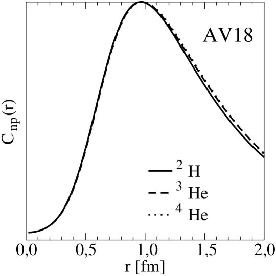
Figure 25: Comparison of the neutron-proton radial correlations in the deuteron, ${}^{3}He$ and ${}^{4}He$ [160].

This shows that, although the 3- and 4-nucleon calculations needed to extract such correlations are very complicated, they result in some simplicities. Possibly comparisons of correlations within few quark systems could lead to similar simplifications and so enhance our understanding of such systems. The work in Ref. [61] for the $QQq$ system is a step in this direction.

In Sec. 9 the charge and matter distributions of the $\bar{q}$ in the $Q\bar{q}$ system ( $\approx B$-meson) were measured and attempts made to fit these distributions with simple functions in Subsec. 3 and also by using the Dirac equation in Subsec. 3. The latter can be viewed in two ways:

1. As simply an alternative form of parametrization of the two distributions with no physical interpretation of the parameters needed.

2. As the construction of an EPT, in which the parameters do have a physical interpretation — albeit phenomenological — on which extensions to multiquark systems can be based.

This leads us to the main problem of how to set up an EPT in order to understand multiquark systems. In the past the key word has been “mimicing”, in which models based on potentials have been mimicing the successful models of multi-nucleon systems. Unfortunately, since such models aim directly at the experimental data, they may be attempting to describe some mechanisms that are outside the scope of the model. This I have called the Nuclear-Physics-Inspired-Approach (NPIA) and it would correspond to Option 1 in the comparison

NPIA $\stackrel{{\scriptstyle 1}}{{\longleftrightarrow}}$ Experimental Data versus Lattice data $\stackrel{{\scriptstyle 2}}{{\longleftrightarrow}}$ QCDIA

However, I believe it is more reasonable to try to create QCD-Inspired-Approaches (QCDIA) as in Option 2. Here the models attempt to mimic directly details of the lattice data that have been obtained under “controlled conditions” and so, hopefully, do not contain undesirable processes not included in the model. In this way the data have a better chance of deciding the form of the model. In contrast, with the NPIA the form of the model tends to be decided beforehand with the experimental data only leading to a tuning of the parameters. An example of this was demonstrated by Fig. 23. There it was seen that using only $(Q\bar{Q})$ correlations did not lead to a flattening of the interquark potential $V(Q\bar{Q})$ — even though such a flattening should arise with the onset of $(Q\bar{q})$ and $(\bar{Q}q)$ mesons being created. Therefore, for an understanding of $V(Q\bar{Q})$ this defect was considered to be a negative feature, since this implementation of LQCD clearly did not agree with experiment. However, for model building this could be envisaged as a positive feature, since LQCD is now generating exact data from the QCD Lagrangian that can be interpreted by a model that is simply a linearly rising potential between a single $Q$ and a single $\bar{Q}$. This intermediate stage model could, hopefully, be more easily extended to the real life situation, when the more complicated correlations in Fig. 22 are treated by LQCD. This intermediate stage could be considered as yet another example of the “unphysical worlds” discussed in Sec. 2 in the context of models with different numbers of colours, spatial dimensions, quark masses etc.. This recalls my earlier work in ${}^{18}O$[162, 163]. There the “real” ${}^{18}O$ needed to be described by “4-particle 2-hole” states in addition to the usual “2-particle 0-hole” states. This is analogous to the matrix of correlations in Fig. 22. It would have been very useful if there had been an “experimental phase” of ${}^{18}O$ that only needed 2-particle 0-hole states for its description. In that case the model for “real” ${}^{18}O$ would have had less freedom.

So far the QCDIA has only been attempted for the $[(Q\bar{q})(Q\bar{q})]$ configuration in Sec. 10. There the $(Q\bar{q})$ lattice data in Fig. 18 was first fitted with a Schrödinger equation to give an effective light quark mass $m_{q,\ {\rm effective}}\approx 400$ MeV. Using a variational method, this Schrödinger approach was then easily extended to the $Q^{2}\bar{q}^{2}$ system using the same interquark potential and $m_{q,\ {\rm effective}}$ determined earlier from the $Q\bar{q}$ data. In principle, this could be extended to any system that can be described in terms of interacting quark clusters.

The problem with the above QCDIA is that it usually results in an $m_{q,\ {\rm effective}}\ll 1$ GeV suggesting the need for a more relativistic approach. This can be attempted at different levels:

1. At the one extreme we can use directly the Dirac equation to describe, say, the $Q\bar{q}$ system as in Subsec. 3. This had some success but we are then confronted with the problem of extending the comparison to multi-quark systems — a second step (2) that is not directly possible for systems containing more than one light quark i.e.

   Lattice data for $Q\bar{q}$ $\stackrel{{\scriptstyle 1}}{{\longrightarrow}}$ 1-quark Dirac Eq. $\stackrel{{\scriptstyle 2\ ??}}{{\longrightarrow}}$ Multi-quark case

2. Use some Semirelativistic Schrödinger-like Equation (SRSE) as described in Subsec. 3. This is most easily formulated in momentum space with the kinetic energy $E_{NR}=m_{q,e}+p^{2}/2m_{q,e}$ being replaced by $E_{R}=\sqrt{p^{2}+m_{q,e}^{2}}$, where $m_{q,e}$ is an effective quark mass chosen to fit some piece(s) of experimental or lattice data. However, care must be taken to treat the potential terms to the same semirelativistic degree by inserting appropriate factors of $m_{q,e}/E_{p}$ as in the Blankenbecler–Sugar equation [35]. The second step (2) to multiquark systems is then probably possible i.e.

   Lattice data for $Q\bar{q}$ $\stackrel{{\scriptstyle 1}}{{\longrightarrow}}$ SRSE $\stackrel{{\scriptstyle 2}}{{\longrightarrow}}$ Multi-quark case

3. Thirdly, a compromise model emerges. First the $Q\bar{q}$ lattice data is fitted by a Dirac equation. This equation then generates other observables that are interpreted in terms of a SRSE, which can be extended to multi-quark systems. This is similar to the philosophy of Bhaduri and Brack [30], who show how the Schrödinger equation with a quark effective mass of $m_{q,\ {\rm effective}}\approx 500$ MeV is able to explain some of the results — energies and magnetic moments — of a Dirac equation for a zero mass quark i.e. they make the comparison

   Lattice data for $Q\bar{q}$ $\stackrel{{\scriptstyle 1}}{{\longrightarrow}}$ Dirac Eq. $\stackrel{{\scriptstyle 2}}{{\longrightarrow}}$ SRSE $\stackrel{{\scriptstyle 3}}{{\longrightarrow}}$ Multi-quark

So what are the “Bridges from Lattice QCD to Nuclear Physics” as advertized in the title of this chapter? So far, the only clear examples involve mainly static (or heavy) quarks ($Q$) as in the extraction of the string energy and the lattice spacing from $V_{QQ}$ with a non-relativistic Schrödinger equation (Sec. 2) and the energies of the various $Q^{4}$ geometries in Secs. 3–7. The introduction of light quarks as in the $(Q\bar{q})$, $[(Q\bar{q})(Q\bar{q})]$ and $[(Q\bar{q})(\bar{Q}q)]$ systems in Secs. 8 – 11 leads to major complications and the only partial success is the Schrödinger description of the $(Q\bar{q})+[(Q\bar{q})(Q\bar{q})]$ energies in Sec. 10. The real test of whether any “Bridge” exists is only now becoming possible with the advent of the lattice data for radial distributions, since such distributions are also at the centre of much of Nuclear Physics. Of course, the final outcome could be that there is no useful bridge for treating multiquark systems in the way we treat multinucleon systems. This would mean that Lattice QCD would only ever be able to directly address problems involving a few quarks — perhaps upto the six quarks needed for the nucleon-nucleon interaction — but not show a general way for how to deal with multiquark systems. This would result in the two worlds of QCD and Nuclear Physics having little direct connection with each other.

However, before such a pessimistic view is adopted, we should remember that Nuclear Physics earlier had another two-world structure that lasted for many years. Until the 1960’s there were essentially two models for the nucleus — the collective liquid-drop-like model that rarely mentioned the nucleon-nucleon potential and, in contrast, the shell model based on this potential. But with the advent of Brueckner theory it was shown how effective interactions in many-nucleon systems could be constructed from the basic nucleon-nucleon potential. This was followed up by the generation of collective effects as interacting particle-hole states [164]. In this way a bridge was made between the basic nucleon-nucleon potential and collectivity — but it took many years.

Acknowledgements

The author wishes to thank Mika Jahma, Jonna Koponen, Timo Lähde and Slawek Wycech for their invaluable help in preparing and commenting on this manuscript. The author, in his rôle as Editor, also wishes to thank the other contributors to this Volume. Without their cooperation and enthusiasm the volume would never have appeared.

Appendix A: Extensions of the $f$-Model from $2\times 2$ to $6\times 6$

A.1: The $3\times 3$ extension of the unmodified two-body approach of Subsec. 1

Because the colour group considered so far is SU(2), there is no distinction between the group properties of quarks ($Q$) and antiquarks ($\bar{Q}$). Four such quarks can then be partitioned as pairs in three different ways

$$A=(Q_{1}Q_{3})(Q_{2}Q_{4}),\ \ B=(Q_{1}Q_{4})(Q_{2}Q_{3})\ \ {\rm and}\ \ C=(Q_{1}Q_{2})(Q_{3}Q_{4}),$$ (A.1)

where each $(Q_{i}Q_{j})$ is a colour singlet. However, these three basis states are not orthogonal to each other. Also, remembering the fact that the quarks are indeed fermions gives, in the weak coupling limit, the condition in the Appendix of Ref. [52]

$$|A\rangle+|B\rangle+|C\rangle=0.$$ (A.2)

Since $\langle A|A\rangle=\langle B|B\rangle=\langle C|C\rangle=1$, we get — in this limit — the equalities
$\langle A|B\rangle=\langle B|C\rangle=\langle A|C\rangle=-1/2$.

In SU(3) the partitioning problem is different since in that case the three partitions are

$$A=(Q_{1}\bar{Q}_{3})(Q_{2}\bar{Q}_{4}),\ \ B=(Q_{1}\bar{Q}_{4})(Q_{2}\bar{Q}_{3})\ \ {\rm and}\ \ C=[(Q_{1}Q_{2})^{d}(\bar{Q}_{3}\bar{Q}_{4})^{d}],$$ (A.3)

where state $C$ is expressed in terms of either colour antitriplet ($d=\bar{3}$) or sextet ($d=6$) states and so cannot appear asymptotically as two clusters.

If all three basis states in SU(2) are included, then the matrix below is singular for the obvious reason that $|A\rangle+|B\rangle+|C\rangle=0$ i.e.

$$\rm{det}\ {\bf N}=\rm{det}\left(\begin{array}[]{ccc}1&-1/2&-1/2\\ -1/2&1&-1/2\\ -1/2&-1/2&1\end{array}\right)=\rm{det}\left(\begin{array}[]{ccc}1&1/2&1/2\\ 1/2&1&-1/2\\ 1/2&-1/2&1\end{array}\right)=0.$$ (A.4)

Earlier this was interpreted to mean that it was unnecessary to include all three states and so the symmetry was broken by keeping the two states with the lowest energy, let us say , $A$ and $B$. A similar effect also occurred in the lattice simulations. There it was found that the energy of the lowest state was always the same in both a $2\times 2$ and $3\times 3$ description, providing $A$ or $B$ had the lowest energy of the three possible partitions. In addition the energy of the second state was, in most cases, more or less the same – the largest difference occurring with the tetrahedral geometry.

A.2: The $3\times 3$ extension of the $f$-model of Subsec. 2

The $f$-model of Subsec. 2, by incorporating multiquark interactions, had the good feature that, when fitting the data ($E_{0},E_{1}$) for a given square, only a single $\bar{f}$ was necessary to get a reasonable fit to both energies — see Fig. 7. Of course, $\bar{f}$ was dependent on the size of the square, but a reasonable parametrization was

$$f(Ia)=\exp(-b_{s}k_{f}S)\ \ {\rm(Version\ \ Ia)},$$ (A.5)

where $S$ is the area of the square and $k_{f}\approx 0.5$. Earlier in Eq. 0.43 a slightly different notation was used. The original hope was that, with $k_{f}$ determined from the squares and nearby rectangles, the model would automatically also fit other geometries with $S$ being the “appropriate” area contained by the four quarks. When the four quarks lie in a plane, the definition of $S$ is clear. However, in non-planar cases the situation is more complicated. One possibility is to simply take $S$ to be the average of the sum of the four triangular areas defined by the positions of the four quarks i.e. the faces of the tetrahedon. For example, in the notation of Eq. A.1, the appropriate area $S(AB)$ for $f$ is

$$S(AB)=0.5[S(431)+S(432)+S(123)+S(124)],$$ (A.6)

where $S(ijk)$ is the area of the triangle with corners at $i,j$ and $k$. For planar geometries this simply reduces to the expected area, but for non-planar cases this is only an approximation to $S(AB)$ – a more correct area being one that is not necessarily a combination of planar areas but of curved surfaces with minimum areas. These possibilities are discussed in Ref. [165]. It would be feasible to incorporate this refinement here, since only a few $(\approx 50)$ such areas are needed for the geometries in Fig. 10. However, for a general situation, in which the positions of the quarks are integrated over, it would become impractical to use the exact value of $S(AB)$, since the expression for the minimum area itself involves a double integration. In contrast, the area used in Eq. A.6 is an algebraic expression and is, therefore, more readily evaluated for any geometry. The above model will be referred to as Version Ia.

This model Ia has only the one free parameter $k_{f}$ in $f({\rm Ia})$ of Eq. A.5. Another possibility with additional parameters $f_{0},\ k_{P}$ is

$$f({\rm Ib})=f_{0}\exp(-b_{s}k_{f}S+\sqrt{b_{s}}k_{P}P)\ \ {\rm(Version\ \ Ib)},$$ (A.7)

where $P$ is the perimeter bounding $S$. This form has been used in Refs. [165]. However, as shown in Ref. [49], this reduces in the continuum limit to the same as Version Ia — the differences at $\beta=2.4$ being mainly due to lattice artefacts.

Unfortunately, in the $2\times 2$ version both of these models have the feature that, for regular tetrahedra, they are unable to reproduce a degenerate ground state with a non-zero energy, since the two eigenvalues are

$$E_{0}=-\frac{f/2}{1+f/2}[V_{CC}-V_{AA}]\ \ {\rm and}\ \ E_{1}=\frac{f/2}{1-f/2}[V_{CC}-V_{AA}],$$ (A.8)

where, in the notation of Fig. 10, $V_{AA}=v_{13}+v_{24}$ and $V_{CC}=v_{14}+v_{23}$ and so for regular tetrahedra $V_{CC}=V_{AA}$, giving $E_{0}=E_{1}=0$.

Prior to the work on tetrahedra the geometries considered had, at most, two of the three possible partitions being degenerate in energy (e.g. for squares) — see Subsec. 2. In these cases, it is found that the lattice energies $E_{0}$ and $E_{1}$ are essentially the same for the three-basis-state calculation $(A+B+C)$ and those two-basis-state calculations ($A+B,\ A+C$ and effectively $B+C$) which involve the basis state with the lowest unperturbed energy. This is one of the reasons why the $2\times 2$ version of the $f$-model in Eq. 0.38 was quite successful for a qualitative understanding of these cases. However, for tetrahedra and the neighbouring geometries calculated in Subsec. 6, it now seems plausible to extend the $f$-model to the corresponding $3\times 3$ version of

$$\left[{\bf V}(f)-\lambda_{i}(f){\bf N}(f)\right]\Psi_{i}=0,$$ (A.9)

in which

$${\bf N}(f)=\left(\begin{array}[]{ccc}1&f/2&f^{\prime}/2\\ f/2&1&-f^{\prime\prime}/2\\ f^{\prime}/2&-f^{\prime\prime}/2&1\end{array}\right)\ \ {\rm and}$$ (A.10)

$${\bf V}(f)=\left(\begin{array}[]{ccc}v_{13}+v_{24}&fV_{AB}&f^{\prime}V_{AC}\\ fV_{BA}&v_{14}+v_{23}&-f^{\prime\prime}V_{BC}\\ f^{\prime}V_{CA}&-f^{\prime\prime}V_{CB}&v_{12}+v_{34}\end{array}\right),$$ (A.11)

where the negative sign in the BC matrix elements is of the same origin as the one in Eqs. 0.51 and A.4.

This apparently leads to the need for two more factors $f^{\prime},f^{\prime\prime}$ defined by

$$\langle A|C\rangle=-f^{\prime}/2\ \ {\rm and}\ \ \langle B|C\rangle=-f^{\prime\prime}/2.$$ (A.12)

However, with the parametrizations of $f$ as in Eqs. A.5 or A.7 and the definition of $S$ as in Eq. A.6, it is seen that $f^{\prime}=f^{\prime\prime}=f$, since $S$ is simply proportional to the area of the faces of the tetrahedron defined by the four quark positions and is independent of the state combination used. Therefore, the $3\times 3$ model has for all 4-quark geometries a form where the $N$ and $V$ matrices are

$${\bf N}(f)=\left(\begin{array}[]{ccc}1&f/2&f/2\\ f/2&1&-f/2\\ f/2&-f/2&1\end{array}\right)\ \ {\rm and}\ \$$ (A.13)

$${\bf V}(f)=\left(\begin{array}[]{ccc}v_{AA}&fV_{AB}&fV_{AC}\\ fV_{BA}&v_{BB}&-fV_{BC}\\ fV_{CA}&-fV_{CB}&v_{CC}\end{array}\right).$$ (A.14)

This extension from $2\times 2$ to $3\times 3$ has the good feature that all three basis states are now treated on an equal footing. This is convenient when considering some general four-quark geometry, since it is then not necessary to choose some favoured $2\times 2$ basis, which could well change as the geometry develops from one form to another. In the weak coupling limit (i.e. $f\rightarrow 1$) the $3\times 3$ matrix in Eq. A.13 becomes the singular matrix in Eq. A.4. However, in this limit, each of the $2\times 2$ matrices corresponding to the three possible partitions A+B, A+C and B+C gives the same results. Away from weak coupling the $3\times 3$ matrix is no longer singular, but now the three possible $2\times 2$ partitions do not necessarily give the same results. In addition to this general problem as $f\rightarrow 1$, there are also the following more specific unpleasant features:

1. For regular tetrahedra all eigenvalues are zero as in the $2\times 2$ models. The reason for this is clear. There is only one energy scale in the model, since all the $v_{ij}$ are the same. Therefore, there can not be any excitations.

2. For a linear geometry, since the “appropriate” area as defined by Eq. A.6 vanishes, we get $f=1$ i.e. we are back to the weak coupling limit and a singular matrix.

3. For squares the model gives $E_{1}=-E_{0}$, whereas the predictions of the $2\times 2$ version in Eqs. A.8 seem to be nearer the lattice data.

4. The differences between using the various combinations of the three partitions are often considerably larger than in the corresponding lattice calculation.

The most glaring problem is the fact that the $3\times 3$ model for the tetrahedron gives three degenerate states with zero energy, because there is only one scale in the model. It is, therefore, necessary to introduce a second energy scale. However, any improvements in the model have very limited choices, since there are only two different matrix elements involved — the diagonal ones all equal to $-E$ and the off-diagonal ones all equal to $\pm 0.5fE$. Therefore, the most general modifications are to change the diagonal matrix elements to $d_{1}-E$ and the off-diagonal ones to $\pm 0.5f(d_{2}-E)$. This results in the eigenvalues

$$E_{0}=E_{1}=\frac{d_{1}+0.5fd_{2}}{1+0.5f}\ \ {\rm and}\ \ E_{2}=\frac{d_{1}-fd_{2}}{1-f}.$$ (A.15)

At first sight it may appear that there is sufficient information to now extract the new parameters $d_{1,2}$, since $f$ can be estimated using the parameters (assumed to be universal) from other geometries — thus leaving two equations for $E_{0,1}$ and $E_{2}$ and the two unknowns $d_{1,2}$. However, as said before, this is too much to demand from the $f$-model, since in the lattice calculation the third basis state in the complete A+B+C basis generally plays a minor rôle in determining the values of $E_{0,1}$ and, therefore, the third eigenvalue is presumably dominated by an excitation of the gluon field. Furthermore, it is of interest to see that a similar feature now arises with $E_{2}$ in Eq. A.15, since this third state is removed in the weak coupling limit i.e. $E_{2}\rightarrow\infty$ as $f\rightarrow 1$. However, in its present form, the $f$-model is only expressed in terms of the lowest energy gluon configurations, since the gluon field is not explicitly in its formulation, but only appears implicitly in the form of the two-quark potentials and the $f$-factors. But already at this stage we see from the behaviour of $E_{2}$ that the effect of excited gluon states seem to be playing a rôle — the topic of the next subsection when the model is further extended to a $6\times 6$ version. In view of this, no quantitative attempt should be made to identify the second excited state emerging from the lattice calculation as $E_{2}$ in this $3\times 3$ version of the $f$-model.

In Ref. [102] it was shown that the two-state model of Eqs. 0.38 with the overlap factor $f=1$ agreed with perturbation theory up to fourth order in the quark–gluon coupling [i.e. to $O(\alpha^{2})$] and gave $E_{0,1}$=0 for tetrahedra. Therefore, the non-zero lattice results for small tetrahedra must be of $O(\alpha^{3})$ at least. Another aspect of this special situation for tetrahedra is also seen — when extracting or interpreting the value of $E_{1}$ — by the need for the third basis state both in the lattice calculation and in the $f$-model, since in comparison with Eq. A.15 the two-basis-state version gives

$$E_{0}=\frac{d_{1}+0.5fd_{2}}{1+0.5f}\ \ {\rm and}\ \ E_{1}=\frac{d_{1}-0.5fd_{2}}{1-0.5f}$$ (A.16)

i.e. both the two- and three- basis-state models have the same ground state, but the former does not show the $E_{0}=E_{1}$ degeneracy.

The expressions in Eq. A.15 are not particularly useful unless there is a model for the parameters $d_{1,2}$. However, since it is not the purpose at this stage to make a comprehensive study of models covering all the 4-quark geometries considered in earlier works [52, 86, 87, 88], only a few general remarks will be made here for the tetrahedron geometry. Models for the $d_{1,2}$ need extensions of the potential in Eq. 0.31, so that for the tetrahedron two energy scales arise. Here several ways of achieving this goal are suggested:

The effect of an isoscalar two-quark potential.
As discussed in Ref. [87], an isoscalar potential $w_{ij}$ can be introduced into $V_{ij}$ — still ensuring $V_{ij}=v_{ij}$ for a colour singlet two-quark system — by extending the form in Eq. 0.6 to

$$V_{ij}=-\frac{1}{3}{\bf\tau}_{i}\cdot{\bf\tau}_{j}\left(v_{ij}-w_{ij}\right)+w_{ij}.$$ (A.17)

In this case, $d_{1}=d_{2}=4w$, since all of the $w_{ij}$ are now equal to $w$ and results in $E_{0}=E_{1}=E_{2}=4w$. Therefore, here $w$ takes on values that range from –0.0035 to –0.0070 i.e. they have values much smaller than the corresponding $v_{ij}=v$ in Eq. 0.31. A similar feature was found in Ref. [87], when the form in Eq. A.17 was introduced to improve the model fit for squares and rectangles. However, as shown in Ref. [102], in perturbation theory all terms of $O(\alpha^{2})$ are included in the two state model of Eq. 0.38 with $f=1$. Therefore, in the weak coupling limit $w_{ij}$ must be of $O(\alpha^{3})$ at least.

The effect of a three- or four-body potential.
The $f$ factor is itself a four-body operator. However, it is conceivable that additional multiquark effects arise. Some perturbative possibilities are discussed in Ref. [102]. There it is shown that all three-quark terms arising from three gluon vertices always vanish, but that the four-gluon vertex can contribute to 2-, 3- and 4-quark terms at $O(\alpha^{3})$. However, in the tetrahedral case ($r=d$), cancellations result in this particular 4-quark term also vanishing.

The effect of non-interacting three gluon exchange processes.
These are also discussed qualitatively in Ref. [102] and contribute at $O(\alpha^{3})$ to 2-, 3- and 4-quark potentials.

The effect of two quark potentials where the gluon field is excited.
The first excited state [$V^{*}(r)$] of the two-quark potential $V(r)$ is approximately given by $V^{*}(r)\approx V(r)+\pi/r$ — see for example Refs. [90, 91]. Therefore, if a fourth state, based on such an excited state, is introduced into the model, it will give attraction in the ground state, since it is higher in energy than the three degenerate basis states so far considered. Furthermore, as the size of the tetrahedron increases this fourth state will approach the other three states, so that the attraction felt in the ground state will increase — a trend seen in the tetrahedron results for $E_{0,1}$ in Fig. 11. This possibility will be discussed more in the $6\times 6$ extension below.

The above isoscalar potential option now offers a reason for $E_{0}=E_{1}\not=0$. But, unfortunately, $E_{2}$ is still equal to $E_{0,1}$ since $d_{1}=d_{2}$. However, there is no reason to expect any three or four body forces to also be purely isoscalars. In this case, their contributions to $d_{1}$ and $d_{2}$ could be different and through the presence of the $(1-f)$ factor in Eq. A.15 any estimates of $E_{2}$ could be very model dependent.

A.3: The $6\times 6$ extension of the $f$-model of Subsec. 2

The above models both have trouble in describing regular tetrahedra. In Refs. [108, 109] an attempt is made to overcome this problem. An interesting feature of the regular tetrahedron data is that the lowest state becomes more bound as the tetrahedron increases in size with the magnitude of $E_{0}$ increasing from –0.0202(8) to –0.028(3) as the $d^{3}$ cube containing the tetrahedron increases from $d=2$ to $d=4$. This is opposite to what happens with squares, where the magnitude of $E_{0}$ decreases from $-0.0572(4)$ to $-0.047(3)$ as $d$ increases from 2 to 5. This indicates that there could be coupling to some higher state(s) that becomes more effective as the size increases and suggests that these higher states contain gluon excitation with respect to the $A,B,C$ configurations. Therefore, the $3\times 3$ model in the previous subsection is further extended to a $6\times 6$ model by adding three more states $A^{*},B^{*},C^{*}$, where in analogy with Eq. A.1

$$A^{*}=(Q_{1}Q_{3})_{E_{u}}(Q_{2}Q_{4})_{E_{u}}\ \ etc..$$ (A.18)

Here $(Q_{1}Q_{3})_{E_{u}}$ denotes a state where the gluon field is excited to the lowest state with the symmetry of the $E_{u}$ representation of the lattice symmetry group $D_{4h}$. Because it is an odd parity excitation, $A^{*},B^{*},C^{*}$ must contain two such states in order to have the same parity as $A,B,C$. The excitation energy of an $E_{u}$ state over its ground state ($A_{1g}$) counterpart is $\approx\pi/r$ for two quarks a distance $r$ apart. As $r$ increases this excitation energy decreases making the effect of the $A^{*},B^{*},C^{*}$ states more important, leading to the effect mentioned above. Here we have assumed that these states arise from a combination of excited states with $E_{u}$. However, it is possible that they involve other excitations, e.g.

$$A^{*}=(Q_{1}Q_{3})_{A^{\prime}_{1g}}(Q_{2}Q_{4})\ \ etc.,$$ (A.19)

where the $A^{\prime}_{1g}$ state is a gluonic excitation with the same quantum numbers as the ground state ($A_{1g}$). For this case the following formalism would be essentially the same. Another possibility, which is not considered here, is that the relevant excitations are flux configurations where all four quarks, instead of two, are involved in forming a colour singlet. In the strong coupling approximation such states would reduce to two-body singlets due to Casimir scaling of the string tensions, namely, the string tension for a higher representation would be more than double the value of the fundamental string tension, thus preventing junctions of two strings in the fundamental and one in the higher representation. This would happen both in SU(2) and SU(3), the only exception being the unexcited $C$ state in SU(3), which would involve an antitriplet string — see Eq. A.3.

For the regular tetrahedral case, in addition to $f=f^{\prime}=f^{\prime\prime}$, there are now several new matrix elements that need to be discussed for ${\bf N(f)}$ and ${\bf V(f)}$ (Eqs. A.9–A.11):

a) With the inclusion of the $A^{*},B^{*},C^{*}$ states and the antisymmetry condition $|A^{*}\rangle+|B^{*}\rangle+|C^{*}\rangle=0$ analogous to Eq. A.2, there are now two more gluon overlap functions $f^{a,c}$ defined as

$$\langle A^{*}|B^{*}\rangle=\langle A^{*}|C^{*}\rangle=\langle B^{*}|C^{*}\rangle=-f^{c}/2\ \ {\rm and}\ \$$

$$\langle A^{*}|B\rangle=\langle A^{*}|C\rangle=..\ \ etc.\ \ ..=-f^{a}/2.$$ (A.20)

Here it is assumed that $f^{a,c}$ are both dependent on $S$ as defined in Eq. A.6. Since $f^{c}$ involves only the excited states, it is reasonable to expect it has a form similar to $f$ in Eq. A.5 i.e.

$$f^{c}=\exp(-b_{s}k_{c}S).$$ (A.21)

b) By orthogonality $\langle A|A^{*}\rangle=\langle B|B^{*}\rangle=\langle C|C^{*}\rangle=0$

c) In the weak coupling limit, from the $|A^{*}\rangle+|B^{*}\rangle+|C^{*}\rangle=0$ condition, we expect $\langle A|B^{*}\rangle=\langle B|C^{*}\rangle=.....=0$ at small distances. To take this into account $f^{a}$ is parametrized as

$$f^{a}=(f^{a}_{1}+b_{s}f^{a}_{2}S)\exp(-b_{s}k_{a}S).$$ (A.22)

If all three parameters $f^{a}_{1},f^{a}_{2},k_{a}$ are varied, it is found that $f^{a}_{1}$ is always consistent with zero — as expected from the above condition that $\langle A|B^{*}\rangle=....=0$. Therefore, usually $f^{a}_{1}$ is fixed at zero.

d) For the potential matrix ${\bf V(f)}$ the diagonal matrix elements, after the lowest energy $V_{DD}$ amongst the basis states is removed, are

$$\langle A^{*}|V-V_{DD}|A^{*}\rangle=v^{*}_{13}+v^{*}_{24}-V_{DD},\ \ etc.,$$

where $V_{DD}={\rm min}[V_{AA}=v_{13}+v_{24},V_{BB}=v_{14}+v_{23},V_{CC}=v_{12}+v_{34}]$ and $v^{*}_{ij}\approx v_{ij}+\pi/r$ is the potential of the excited $E_{u}$ state, which is a quantity also measured on the lattice along with the four-quark energies.

In the special case of regular tetrahedra $V_{DD}=V_{AA}=V_{BB}=V_{CC}$ and ${\bf V}$ reduces to the form

$${\bf V}=\left[\begin{array}[]{ccc|ccc}V_{AA}&-fV_{AA}/2&-fV_{AA}/2&0&-f^{a}V_{a}/2&-f^{a}V_{a}/2\\ -fV_{AA}/2&V_{AA}&-fV_{AA}/2&-f^{a}V_{a}/2&0&-f^{a}V_{a}/2\\ -fV_{AA}/2&-fV_{AA}/2&V_{AA}&-f^{a}V_{a}/2&-f^{a}V_{a}/2&0\\ \hline\cr 0&-f^{a}V_{a}/2&-f^{a}V_{a}/2&V_{b}&-f^{c}V_{c}/2&-f^{c}V_{c}/2\\ -f^{a}V_{a}/2&0&-f^{a}V_{a}/2&-f^{c}V_{c}/2&V_{b}&-f^{c}V_{c}/2\\ -f^{a}V_{a}/2&-f^{a}V_{a}/2&0&-f^{c}V_{c}/2&-f^{c}V_{c}/2&V_{b}\\ \end{array}\right],$$ (A.23)

where $V_{a}\ ,\ V_{b}\ ,\ V_{c}$ can be expressed in terms of $V_{AA}$ and $v^{*}(ij)$ plus some fine tuning parameters. As with all geometries

$${\bf N}=\left[\begin{array}[]{ccc|ccc}1&-f/2&-f/2&0&-f^{a}/2&-f^{a}/2\\ -f/2&1&-f/2&-f^{a}/2&0&-f^{a}/2\\ -f/2&-f/2&1&-f^{a}/2&-f^{a}/2&0\\ \hline\cr 0&-f^{a}/2&-f^{a}/2&1&-f^{c}/2&-f^{c}/2\\ -f^{a}/2&0&-f^{a}/2&-f^{c}/2&1&-f^{c}/2\\ -f^{a}/2&-f^{a}/2&0&-f^{c}/2&-f^{c}/2&1\\ \end{array}\right].$$ (A.24)

The full $6\times 6$ matrix $[{\bf V}-(E+V_{AA}){\bf N}]$ now factorizes into three $2\times 2$ matrices, two of which are identical – giving the observed degeneracy. These two matrices have determinants of the form

$$\left|\begin{array}[]{cc}-E(1+f/2)&-f^{a}(E-V_{a})/2\\ -f^{a}(E-V_{a})/2&\ \ -E(1+f^{c}/2)+V_{b}+f^{c}V_{c}/2\\ \end{array}\right|=0,$$ (A.25)

whereas the third $2\times 2$ matrix has the determinant

$$\left|\begin{array}[]{cc}-E(1-f)&f^{a}(E-V_{a})\\ f^{a}(E-V_{a})&\ \ -E(1-f^{c})+V_{b}-f^{c}V_{c}\\ \end{array}\right|=0.$$ (A.26)

In this case the problem reduces to solving two quadratic equations for $E$. However, away from the regular tetrahedron the complete 6$\times$6 matrix needs to be treated directly.

By fitting simultaneously the energies $E_{0}$ and $E_{1}$ from the lattice results for the geometries in Fig. 10 an interquark potential model can be constructed that is able to explain, on the average, these energies. The full model utilized 6 basis states $A,B,C,A^{*},B^{*},C^{*}$ and in its most general form has eight parameters. However, in practice, only 3 of these ($k_{f},k_{a},f^{a}_{2}$) need be considered as completely free when fitting the data.

The parameters that are of most interest are those connected with the ranges of the various interactions, namely, $k_{f}$ and $k_{a}$. Here “range” is defined as $r_{f,a,c}=\sqrt{1/b_{s}k_{f,a,c}}$. In the $2\times 2$ version, where $k_{a}$ is effectively infinite, we get $k_{f}({\rm Ia})$=0.57(1) i.e. $r_{f}({\rm Ia})=5.0$ in lattice units of 0.12 fm. However, when the excited states $A^{*},B^{*},C^{*}$ are introduced, the interaction between the basic states $A,B,C$ decreases by raising $k_{f}$ to 1.51 giving $r_{f}=3.1$. But at the same time this loss of binding by the direct interaction between $A,B,C$ is compensated by their coupling to the $A^{*},B^{*},C^{*}$ states. This coupling in Eq. A.22 is found to have about the same range $r_{a}=5.1$ as $r_{f}({\rm Ia})$ in Eq. A.5, whereas the direct interaction between the $A^{*},B^{*},C^{*}$ states seems, in all fits, to be satisfied with simply a two-quark description without any four-quark correction (i.e. $k_{c}$=0) in Eq. A.21. The observation that $r_{f}({\rm Ia})\approx r_{a}$ suggests that the energy density has a range dictated by the longest range available — namely $r_{a}$. Therefore, when the $A^{*},B^{*},C^{*}$ states are not explicitly present, as in Model Ia, the only available range $r_{f}({\rm Ia})$ has to simulate the rôle of $r_{a}$. In the binding energies the contributions from the $A^{*},B^{*},C^{*}$ states rapidly dominate over those from the $A,B,C$ states. For example, with squares of side $R$, the $A,B,C$ states contribute only 85, 40, 10% to the binding energy for $R$=2,4,6 respectively. Of course, at the largest distances ($\approx 0.7$ fm) the quenched approximation is expected to break down and the rôle of quark-pair creation to become important.

Appendix B: Extension of the $f$-Model to $[(Q\bar{q})(Q\bar{q})]$ Systems

When only two of the four quarks are static the corresponding matrices for $Q({\bf r_{1}})Q({\bf r_{2}})\bar{q}({\bf r_{3}})\bar{q}({\bf r_{4}})$ can be expressed in a similar form but where the matrix elements are now integrals over the positions of the two light antiquarks. In the notation of Fig. 4 we consider basis state $A$ to be the one realised as two separate heavy-light mesons — $[Q_{1}\bar{q}_{3}]$ and $[Q_{2}\bar{q}_{4}]$ — when the distance ${\bf R}={\bf r_{1}}-{\bf r_{2}}$ between the two heavy quarks becomes large. In this state the convenient coordinates are then ${\bf s_{1}}={\bf r_{3}}-{\bf r_{1}}$ and ${\bf s_{2}}={\bf r_{4}}-{\bf r_{2}}$, whereas for the other partition $B$ the convenient coordinates are ${\bf t_{1}}={\bf r_{3}}-{\bf r_{2}}={\bf s_{1}}+{\bf R}$ and ${\bf t_{2}}={\bf r_{4}}-{\bf r_{1}}={\bf s_{2}}-{\bf R}.$

To describe this system in terms of an Effective Potential Theory the three ingredients quoted in Subsec. 2 are needed — see Ref. [60] for more details of the specific example now to be described:

A wave equation.
For simplicity, the system is considered to be non-relativistic resulting in a Schrödinger-like equation

$$|{\bf K}^{\prime}(R)+{\bf V}^{\prime}(R)-E(4,R){\bf N}^{\prime}(R)|\psi=0$$ (B.1)

i.e. a Resonating Group equation as discussed by Oka and Yazaki in Chapter 6 of Ref. [36] and also Ref. [37]. This is a generalisation of Eq. 0.37 to non-static quarks and can be solved using a variational wave function taken to have the form [140]

$$\psi({\bf r_{i}},f)=f^{1/2}({\bf r_{1}},{\bf r_{2}},{\bf r_{3}},{\bf r_{4}})\sum^{N_{4}}_{i=1}\exp(-\tilde{\bf{X}}{\bf M}_{i}\bf{X}),$$ (B.2)

where $\tilde{\bf{X}}=(\bf{s_{1}},\ \bf{s_{2}},\ \bf{R})$ and each matrix $\bf{M}_{i}$ has the form

$${\bf M}_{i}=\frac{1}{2}\left(\begin{array}[]{ccc}a_{i}&b_{i}&c_{i}\\ b_{i}&d_{i}&e_{i}\\ c_{i}&e_{i}&g_{i}\\ \end{array}\right).$$ (B.3)

Since the present problem considers the masses of the light quarks to be equal, it is sufficient to use a simplified form of $\bf{M}_{i}$ with $b_{i}=0,\ d_{i}=a_{i}$ and $e_{i}=c_{i}$. This is not necessary, but it is expected to be the dominant term in such a symmetric case. Already for $N_{4}=2$, this wave function is indeed adequate for giving sufficiently accurate four-quark binding energies. Even this choice involves five free parameters $(a_{1},\ c_{1},\ a_{2},\ c_{2},\ g_{2})$ in the variation – with $g_{1}$ being fixed at unity to set the overall normalisation. In what follows the positions of the light quarks are integrated over leaving matrix elements that are functions of R. In order to achieve this in any practical way it is necessary to have a form for $f({\bf r_{1}},{\bf r_{2}},{\bf r_{3}},{\bf r_{4}})$ that has a simple spatial dependence. Here the very symmetrical form in Eq. 0.44, defined by a single parameter $k_{f}$, is used i.e.

$$f=\exp\big{[}-k_{f}b_{s}\sum\limits_{i<j}r^{2}_{ij}\big{]}$$ (B.4)

(N.B. Here $k_{f}=k/6$, where $k$ was defined in Eq. 0.44.) It should be emphasised that this form of $f$ is purely for numerical simplicity leading to analytical expressions for all matrix elements. As in the static case $k_{f}$ is a free parameter, which should be adjusted to fit the four-quark lattice energies.

The wave function in Eq. B.2 is used for both states $A$ and $B$. This is an approximation that appears to work well for the $Q^{2}\bar{q}^{2}$ system, since $A$ and $B$ are similar in structure for the $R$ values of interest here.

An interquark potential.
This enters in three different contexts:
1) As $v(13),\ v(24),\ v(14),\ v(23)$ in the $V_{Q\bar{q}}$ potential. This is taken to be of the standard form in Eq. 0.6, namely

$$aV(2,r)=-\frac{0.309(38)}{r/a}+0.1649(36)r/a+0.629(25),$$ (B.5)

which gives a string energy of (445 MeV)² for $a=0.18$ fm. This was obtained by fitting $V_{Q\bar{Q}}$ generated on a $16^{3}\times 24$ lattice. Here the emphasis was to get a good fit over the important range of $r\sim(2-4)a$ and is in contrast to the potential in Ref. [51], which was designed to extract the string tension at large values of $r$.
2) As $v(34)$ for the $V_{\bar{q}\bar{q}}$ potential. Here it is assumed to also be of the form in Eq. B.5.
3) As $v(12)$ for the $V_{QQ}$ potential. This was calculated from the same gauge configurations as the four-quark energies. In this case there was no need to fit $V_{QQ}$ with a function of $R$, since it is only ever needed at discrete values of $R$ – the ones for which the four-quark energies are calculated.

An effective quark mass $\mathbf{m_{q}}$.
In this case $m_{q}$ can be determined beforehand by carrying out an EPT analysis of the correponding two-body energies in Fig. 13. Using the potential in Eq. B.5, a value of $m_{q}\approx 400$ MeV is able to give a good fit to the spin-averaged energies with $L=0,\ 1,\ 2$ and 3. However, the results are not strongly dependent on $m_{q}$ — see Fig. 18. A disturbing feature of this result is that $m_{q}\ll 1$ GeV indicating the need for a relativistic approach — as discussed in Sec. 12.

In Eq. B.1 the normalisation matrix ${\bf N}^{\prime}(R,k_{f})$ — a generalisation of ${\bf N}(f)$ in Eq. 0.38 to non-static quarks in SU(3) — can now be written as

$${\bf N^{\prime}}(R,\ k_{f})=\left(\begin{array}[]{ll}N(R,\ 0)&\frac{1}{3}N(R,\ k_{f})\\ \frac{1}{3}N(R,\ k_{f})&N(R,\ 0)\\ \end{array}\right),$$ (B.6)

where, after integrating over $\bf{s_{1}}$ and $\bf{s_{2}}$, $N(R,\ k_{f})$ can be expressed as a sum of terms of the form

$$\frac{\pi^{3}}{(aX)^{3/2}}\exp\left[-(Z-\frac{Y^{2}}{X})R^{2}\right],$$ (B.7)

where $a=0.5(a_{i}+a_{j})+3k_{f}$, $c=0.5(c_{i}\pm c_{j})+2k_{f}$, $d=0.5(c_{i}\pm c_{j})-2k_{f}$, $g=0.5(g_{i}+g_{j})+4k_{f}$, $X=a-k_{f}^{2}/a$, $Y=c+k_{f}d/a$ and $Z=g-d^{2}/a$.

Since two of the quarks are not static there is now also a kinetic energy matrix in Eq. B.1, namely,

$${\bf K^{\prime}}(R,\ k_{f})=\left(\begin{array}[]{ll}K_{3}(R,0)+K_{4}(R,0)&\frac{1}{3}[K_{3}(R,k_{f})+K_{4}(R,k_{f})]\\ \frac{1}{3}[K_{3}(R,k_{f})+K_{4}(R,k_{f})]&\ K_{3}(R,0)+K_{4}(R,0)\\ \end{array}\right),$$ (B.8)

where, for example,

$$K_{3}(R,k_{f})=\int d^{3}s_{1}d^{3}s_{2}\psi^{\star}(k_{f})\left[-\frac{d^{2}}{2m_{q}dr_{3}^{2}}\right]\psi(k_{f}).$$ (B.9)

Again these integrals can be expressed in forms similar to that in Eq. B.7.

Finally, the potential matrix — a generalisation of ${\bf V}(f)$ in Eq. 0.38 to non-static quarks — has the form

$${\bf V^{\prime}}(R,\ k_{f})=\left(\begin{array}[]{ll}\langle v(13),0\rangle+\langle v(24),0\rangle&\ \langle V_{AB},k_{f}\rangle\\ \langle V_{AB},k_{f}\rangle&\langle v(14),0\rangle+\langle v(23),0\rangle\\ \end{array}\right).$$ (B.10)

Here

$$\langle V_{AB},k_{f}\rangle=\langle V_{Q\bar{q}}\rangle-\langle V_{\bar{q}\bar{q}}\rangle-\langle V_{QQ}\rangle,$$

where

$$\langle V_{Q\bar{q}}\rangle= \frac{1}{3}\left[\langle v(13),k_{f}\rangle+\langle v(24),k_{f}\rangle+\langle v(14),k_{f}\rangle+\langle v(23),k_{f}\rangle\right],$$

$$\langle V_{\bar{q}\bar{q}}\rangle= \frac{1}{3}\langle v(34),k_{f}\rangle\ \ \ {\rm and}\ \ \ \langle V_{QQ}\rangle=\frac{1}{3}N(R,k_{f})V(2,R).$$ (B.11)

Here $N(R,k_{f})$ is defined in Eq. B.6, $V(2,R)$ is the potential between the two heavy quarks and, for example,

$$\langle v(13),k_{f}\rangle=\int d^{3}s_{1}d^{3}s_{2}\psi^{\star}(k_{f})V(s_{1})\psi(k_{f}).$$ (B.12)

For potentials of the form in Eq. 0.6, these integrals can be expressed in terms of Error functions. The energy $E(4,R,k_{f})$ of the two heavy-light meson system is then obtained by diagonalising Eq. B.1. Since this equation is a $2\times 2$ determinant, a prediction can also be made for an excited state $E^{*}(4,R,k_{f})$ and the corresponding binding energy $B^{*}(4,R).$

References

- [1] e.g. R. K. Ellis, W.J. Stirling and B. R. Webber, “QCD and collider physics”, (Cambridge University Press, 1996); E. Leader, “An introduction to gauge theories and modern particle physics: Vol. 2 CP-violation, QCD and hard processes”, (Cambridge University Press, 1996); T. Muta, “Foundations of QCD: An introduction to Perturbative Methods in Gauge Theories (2nd Edition)”, World Scientific Lecture Notes in Physics – Vol. 57 (World Scientific, 1998); Y. L. Dokshitzer, Phil. Trans. Roy. Soc. Lond. A359, 309 (2001) hep-ph/0106348; P. Hoyer, Nucl. Phys. A711, 3 (2002), hep-ph/0208181; S. Capitani, Phys. Rept. 382, 113 (2003), hep-lat/0211036
- [2] M. Lüscher, Annales Henri Poincare 4, S197 (2003), hep-ph/0211220; M. Creutz, Nucl. Phys. Proc. Suppl. 94, 219 (2001), Latt00 and hep-lat/0010047; “The Early Days of Lattice Gauge Theory”, hep-lat/0306024; C. Davies, “Lattice QCD”, Lectures given at 55th Scottish Universities Summer School in Physics: Heavy Flavor Physics, St. Andrews, Scotland, (Institute of Physics 2002, eds. C.T.H. Davies and S.M. Playfer, 2001) p.105, hep-ph/0205181; G. Münster and M. Walzl, “Lattice Gauge Theory — a Short Primer”, Published in Zuoz 2000, Phenomenology of gauge interactions p. 127, hep-lat/0012005; T. DeGrand, “Lattice QCD at the end of 2003”, hep-ph/0312241 to be published in Review for Int. J. Mod. Phys. A. (Worldscience)
- [3] S. Aoki et al. Nucl. Phys. Proc. Suppl. 106, 230 (2002)
- [4] M. G. Alford, T. R. Klassen, G.P. Lepage, Phys. Rev. D58, 034503 (1998), hep-lat/9712005; G.P. Lepage, Nucl. Phys. Proc. Suppl. 47, 3 (1996), also Latt95 and hep-lat/9510049
- [5] B. Sheikholeslami and R. Wohlert, Nucl. Phys. B259, 572 (1985)
- [6] M. Lüscher, S. Sint, R. Sommer, P. Weisz and U. Wolff, Nucl. Phys. B491, 323 (1997), hep-lat/9609035
- [7] A. S. Kronfeld, “Uses of Effective Field Theory in Lattice QCD” in: At the Frontiers of Particle Physics: Handbook of QCD, (ed. M. Shifman) 4 Chp. 39, (World Scientific, Singapore, 2002), hep-lat/0205021
- [8] A. S. Kronfeld, eConf C020620:FRBT05 (2002), hep-ph/0209231
- [9] A. C. Irving, Nucl. Phys. Proc. Suppl. 119, 341 (2003), Latt02 and hep-lat/0208065
- [10] qq+q Collaboration, F. Farchioni, C. Gebert, I. Montvay and L. Scorzato, “On the price of light quarks”, hep-lat/0209142
- [11] M. Creutz, “Quarks, Gluons, and Lattices” (Cambridge University, Cambridge, UK, 1983)
- [12] I. Montvay and G. Münster, “Quantum Fields on a Lattice” (Cambridge Monographs on Mathematical Physics, CUP 1994)
- [13] H. J. Rothe, “Lattice Gauge Theories”, World Scientific Lecture Notes in Physics - Vol. 59 (World Scientific Publishing Co., Singapore, 1997)
- [14] C. DeTar and S. Gottlieb, Physics Today, February 2004, 45
- [15] H. Neuberger, “Lattice Field Theory: past, present and future”, hep-ph/0402148
- [16] K. Symanzik, “Recent Developments in Gauge Theories”, edited by G.’t Hooft et al. (Plenum, New York, 1980): Nucl. Phys. B226, 187, 205 (1983).
- [17] J. Gasser and H. Leutwyler, Ann. Phys. 158, 142 (1984): Nucl. Phys. B250, 465 (1985)
- [18] A. W. Thomas, Nucl. Phys. Proc. Suppl. 119, 50 (2003), hep-lat/0208023.
- [19] J. Soto, Quark Confinement and the Hadron Spectrum, Proceedings of the 5th International Conference, Gargnano, Italy, September 2002 (World Scientific 2003) p.227
- [20] N. Brambilla, A. Pineda, J. Soto and A. Vario, Nucl. Phys. B566, 275 (2000); A.Vario, Quark Confinement and the Hadron Spectrum, Proceedings of the 5th International Conference, Gargnano, Italy, September 2002 (World Scientific 2003) p.73
- [21] U. van Kolck, Nucl. Phys. A699, 33 (2002); U. van Kolck, L. J. Abu-Raddad and D. M. Cardamone, nucl-th/0205058; D. Phillips, Czech. J. Phys. 52, B49 (2002), nucl-th/0203040
- [22] J. A. Oller, AIP Conf. Proc. 660, 116 (2003), nucl-th/0207086
- [23] S. Weinberg, Physica A96, 327 (1979); Nucl. Phys. B363, 3 (1991)
- [24] S.C. Pieper and R. B. Wiringa, Ann. Rev. Nucl. Part. Sci. 51, 53 (2001)
- [25] N. Glendenning, “Compact Stars” (Springer, 1996)
- [26] A. Akmal, V. Pandharipande and D. Ravenhall, Phys. Rev. C 58, 1804 (1998)
- [27] R. Machleidt and I. Slaus, J. Phys. G27, R69 (2001), nucl-th/0101056; R. Machleidt, Nucl. Phys. A689, 11 (2001) nucl-th/0009055 : Phys. Rev. C63, 024001 (2001), nucl-th/0006014
- [28] J. L. Richardson, Phys. Lett. 82B, 272 (1979)
- [29] E. Eichten, K. Gottfried, T. Kinoshita, K. D. Lane and T. M. Tan, Phys. Rev. D21, 203 (1980); E. Eichten and F. Feinberg, Phys. Rev. D23, 2724 (1981)
- [30] R. K. Bhaduri and M. Brack, Phys. Rev. D25, 1443 (1982)
- [31] M. Baker, J. S. Ball and F. Zachariasen, Phys. Rev. D51, 1968 (1995)
- [32] P. R. Page, T. Goldman and J. N. Ginocchio, Phys. Rev. Lett. 86, 204 (2001)
- [33] M. Di Pierro and E. Eichten, Phys. Rev. D64, 114004 (2001)
- [34] H. Crater, B. Liu and P. Van Alstine, “Two-Body Dirac Equations”, hep-ph/0306291
- [35] G. E. Brown and A. D. Jackson, “The Nucleon-Nucleon Interaction”, (North–Holland Publishing Co., 1976)
- [36] Editor W. Weise “Quarks and Nuclei”, International Review of Nuclear Physics – Vol. 1 1984 (World Scientific Publishing Co. Pte Ltd 1984)
- [37] T. Sakai, J. Mori, A. J. Buchmann, K. Shimizu and K. Yazaki, Nucl. Phys. A625, 192 (1997), nucl-th/9709054
- [38] M. Oka, “Baryon-Baryon Interaction in the Quark Cluster Model”, hep-ph/0306173
- [39] F. Coester, “From Light Nuclei to Nuclear Matter — The Rôle of Relativity”, nucl-th/0111025; F. Coester and W. N. Polyzou, “Relativistic Quantum Mechanics of Many Body Systems”, nucl-th/0102050
- [40] L. Ya. Glozman and D. O. Riska, Phys. Rep. 268, 263 (1996), hep-ph/9505422: Nucl. Phys. A603, 326 (1996), erratum ibid A620, 510 (1997), hep-ph/9509269
- [41] S. Chernyshev, M. A. Nowak, and I. Zahed, Phys. Rev. D53, 5176 (1996)
- [42] H. Heiselberg and M. Hjorth-Jensen, Phys. Repts. 328, 237 (2000)
- [43] E. Shuryak and D. O. Riska, private communication
- [44] D. H. Perkins, “An Introduction to High Energy Physics” (Addison-Wesley Pub. Co., 1972)
- [45] S. Veseli and M.G. Olsson, Phys. Lett. B383, 109 (1996), hep-ph/9606257
- [46] C. Rebbi, Phys. Repts. 12C, 1 (1974)
- [47] K. Wilson, Phys. Rev. D10, 2445 (1974)
- [48] R. Sommer, Nucl. Phys. B411, 839 (1994), hep-lat/9310022.
- [49] P. Pennanen, Phys. Rev. D55, 3958 (1997), hep-lat/9608147
- [50] UKQCD Collaboration: C. R. Allton et al., Phys. Rev. D49, 474 (1994), hep-lat/9309002
- [51] R. G. Edwards, U. M. Heller and T. R. Klassen, Nucl. Phys. B517, 377 (1998), hep-lat/9711003
- [52] A.M. Green, C. Michael and M.E. Sainio, Z. Phys. C67, 291 (1995), hep-lat/9404004
- [53] A.M. Green, J. Lukkarinen, P. Pennanen and C. Michael, Phys. Rev. D53, 261 (1996), hep-lat/9508002
- [54] N. Isgur and J.E. Paton, Phys. Rev. D31, 2910 (1985)
- [55] M. Baker, J.S. Ball and F. Zachariasen, Phys. Rev. D51, 1968 (1995); Int. J. Mod. Phys. A11, 343 (1996)
- [56] UKQCD Collaboration: C. Michael and J. Peisa, Phys. Rev. D58, 034506 (1998), hep-lat/9802015
- [57] A.M. Green, J. Ignatius, M. Jahma and J. Koponen, work in progress
- [58] A.M. Green, J. Koponen, P. Pennanen and C. Michael, Phys. Rev. D65, 014512 (2002), hep-lat/0105027
- [59] A.M. Green, J. Koponen, P. Pennanen and C. Michael, Eur. Phys. J. C28, 79 (2003), hep-lat/0206015
- [60] A. M. Green, J. Koponen and P. Pennanen, Phys. Rev. D61, 014014 (2000), hep-ph/9902249
- [61] J. Koponen, work in progress
- [62] C. Michael, Phys. Lett. B232, 247 (1989), Nucl. Phys. (Proc. Suppl) B 17, 59 (1990)
- [63] B. Lucini and M. Teper, JHEP 0106, 050 (2001); B. Lucini, M. Teper and U. Wenger, “Features of SU(N) Gauge Theories”, hep-lat/0309170
- [64] M. Teper, Phys. Rev. D59, 014512 (1999); B. Lucini and M. Teper, Phys. Rev. D66, 097502 (2002)
- [65] F. Karsch, Nucl. Phys. B205, 285 (1982)
- [66] G. Burgio et al., Phys. Rev. D67, 114502 (2003), hep-lat/0303005 also Latt03 and hep-lat/0309058, hep-lat/0310036
- [67] CP-PACS, M. Okamoto et al., Phys. Rev. D65, 094508 (2002), hep-lat/0112020
- [68] S. Hashimoto and M. Okamoto, Phys. Rev. D67, 114503 (2003), hep-lat/0302012; S. Sakai and A. Nakamura, “ Improved gauge action on an anisotropic lattice”, hep-lat/0311020
- [69] S. Aoki et al. (CP-PACS), Phys. Rev. Lett. 84, 238 (2000), hep-lat/9904012
- [70] D. B. Leinweber, A. W. Thomas, K. Tsushima and S. V. Wright, Phys. Rev. D61, 074502 (2000), hep-lat/9906027; R. D. Young, D. B. Leinweber, A. W. Thomas and S. V. Wright, Phys. Rev. D66, 094507 (2002), hep-lat/0205017
- [71] S. R. Beane and M. J. Savage, Phys. Lett. B535, 177 (2002), hep-lat/0202013
- [72] S. R. Beane and M. J. Savage, Phys. Rev. D67, 054502 (2003), hep-lat/0210046
- [73] P. Lacock and C. Michael, Phys. Rev. D52, 5213 (1995)
- [74] UKQCD Collaboration: M. Foster and C. Michael, Phys. Rev. D59, 074503 (1999), hep-lat/9810021; M. Foster, University of Liverpool PhD thesis 1998
- [75] S. R. Beane and M. J. Savage, Nucl. Phys. A717, 91 (2003), nucl-th/0208021
- [76] E. Epelbaum, Ulf-G. Meissner and W. Glöckle, Nucl. Phys. A714, 535 (2003), nucl-th/0207089 and nucl-th/0208040
- [77] UKQCD Collaboration: C. Michael and P. Pennanen, Phys. Rev. D60, 054012 (1999), hep-lat/9901007
- [78] M. Lüscher, Commun. Math. Phys. 105, 153 (1986) and Nucl. Phys. B354, 531 (1991)
- [79] S.R. Beane, P.F. Bedaque, A. Parreno and M.J. Savage, “Two nucleons on a Lattice”, hep-lat/0312004
- [80] P. Bedaque, “Aharonov-Bohm effect and nucleon-nucleon phase shifts on the lattice”, nucl-th/0402051
- [81] CP-PACS Collaboration: T. Yamazaki et al., “I=2 Scattering Phase Shift with two Flavors of Improved Dynamical Quarks”, hep-lat/0402025
- [82] I. Wetzorke and F. Karsch, Nucl. Phys. Proc. Suppl. 119, 278 (2003), Latt02 and hep-lat/0208029
- [83] S. Sasaki, “ Lattice study of exotic S=+1 baryon”, hep-lat/0310014; F. X. Lee et al.,“ A search for Pentaquarks on the Lattice”, poster at Lattice 2003 in Tsukuba
- [84] T. Nakano et al., Phys. Rev. Lett. 91, 012002 (2003)
- [85] G. Bali, Phys. Rept. 343, 1 (2001), hep-ph/0001312
- [86] A.M. Green, C. Michael and J.E. Paton, Phys. Lett. B280, 11 (1992)
- [87] A.M. Green, C. Michael and J.E. Paton, Nucl. Phys. A554, 701 (1993), hep-lat/9209019
- [88] A.M. Green, C. Michael, J.E. Paton and M.E. Sainio, Int. J. Mod. Phys. E2, 479 (1993), hep-lat/9301006
- [89] F. Lenz et al., Ann. Phys. (N.Y.) 170, 65 (1986); K. Masutani, Nucl. Phys. A468, 593 (1987)
- [90] S. Perantonis, A. Huntley and C. Michael, Nucl. Phys. B326, 544 (1989)
- [91] S. Perantonis and C. Michael, Nucl. Phys. B347, 854 (1990)
- [92] S.P. Booth et al., Phys. Lett. B275, 424 (1992)
- [93] M. Della Morte et al., “ Static quarks with improved statistical precision”, Latt03 and hep-lat/0309080, hep-lat/0307021
- [94] S. Hashimoto, Phys. Rev. D50, 4639 (1994)
- [95] A. Hasenfratz and F. Knechtli, Phys. Rev. D64, 034504 (2001); A. Hasenfratz, R. Hoffmann and F. Knechtli, Nucl. Phys. B (Proc. Suppl.) 106, 418 (2002)
- [96] K. Choi and W. Lee,“Penguin diagrams for the HYP staggered fermions”, Latt03 and hep-lat/0309070; T. Bhattacharya et al., “Calculating weak matrix elements using HYP staggered fermions”, Latt03 and hep-lat/0309105; S. Bilson-Thompson and W. Lee,“ Description and comparison of Fat7 and HYP fat links”, hep-lat/0310056
- [97] S. Ohta, M. Fukugita and A. Ukawa, Phys. Lett. B173, 15 (1986).
- [98] A.M. Green and J.E. Paton, Nucl. Phys. A492, 595 (1989)
- [99] C. Michael, Phys. Lett. B283, 103 (1992)
- [100] M. B. Gavela et al., Phys. Lett. B82, 431 (1979).
- [101] O. Morimatsu, A. M. Green and J.E. Paton, Phys. Lett. B258, 257 (1991)
- [102] J. T. A. Lang, J. E. Paton and A. M. Green, Phys. Lett. B366, 18 (1996), hep-ph/9508315
- [103] O. Morimatsu, Nucl. Phys. A505, 655 (1989)
- [104] B. Masud, J.E. Paton, A.M. Green and G.Q. Liu, Nucl. Phys. A528, 477 (1991)
- [105] H. Matsuoka and D. Sivers, Phys. Rev. D33, 1441 (1987)
- [106] C. Alexandrou, T. Karapiperis and O. Morimatsu, Nucl. Phys. A518, 723 (1990)
- [107] A.M. Green, G.Q. Liu and S. Wycech, Nucl. Phys. A509, 687 (1990)
- [108] A.M. Green and P. Pennanen, Phys. Lett. B426, 243 (1998), hep-lat/9709124
- [109] A.M. Green and P. Pennanen, Phys. Rev. C57, 3384 (1998), hep-lat/9804003
- [110] C. Bernard et al., Phys. Rev. Lett. 81, 4812 (1998), hep-ph/9806412
- [111] D.E. Groom et al., Review of Particle Physics, Eur. J. Phys. C15, 1 (2000)
- [112] C. Weiser, Proceedings of the 28th International Conference on High Energy Physics, Warsaw 1996, p.531 (Edited by I. Adjuk and A. Wroblewski, World Scientific 1996) — see also http://www-ekp.physik.uni-karlsruhe.de/ weiser/proc_warsaw/index.html
- [113] UKQCD Collaboration: C. McNeile and C. Michael, Phys. Rev. D63, 114503 (2001), hep-lat/0010019
- [114] A.M. Green, J. Koponen, C. McNeile, C. Michael and G. Thompson, Phys. Rev. D69, 094505 (2004), hep-lat/0312007
- [115] H. J. Schnitzer, Phys. Rev. D18, 3482 (1978)
- [116] H. J. Schnitzer, Phys. Lett. B226, 171 (1989)
- [117] C. Alexandrou, Ph. de Forcrand and A. Tsapalis, Phys. Rev. D66, 094503 (2002), hep-lat/0206026
- [118] C. Alexandrou, Ph. de Forcrand and A. Tsapalis, Nucl. Phys. Proc. Suppl. 119, 422 (2003), Latt02 and hep-lat/0209067.
- [119] UKQCD Collaboration: C.R.Allton et al., Phys. Rev. D60, 034507 (1999), hep-lat/9808016
- [120] UKQCD Collaboration: C. McNeile and C. Michael, Phys. Lett. B491, 123 (2000), hep-lat/0006020
- [121] V. D. Mur, V. S. Popov, Yu. A. Simonov and V. P. Yurov, J. Exp. Theor. Phys. 78, 1 (1994), hep-ph/9401203
- [122] M. Lüscher, K. Symanzik and P. Weisz, Nucl. Phys. B173, 465 (1980) M. Lüscher, Nucl. Phys. B180, 317 (1981)
- [123] M. W. Paris, Phys. Rev. C68, 025201 (2003), nucl-th/0305020
- [124] D. S. Kuzmenko and Yu. A. Simonov, Phys. Atom. Nucl. 66, 950 (2003), Yad. Fiz. 66, 983 (2003), hep-ph/0202277 and hep-ph/0302071
- [125] H. Ichie, V. Bornyakov, T. Streuer and G. Schierholz, Nucl. Phys. A721, 899 (2003), hep-lat/0212036 also hep-lat/0304008; H. Suganuma, T.T. Takahashi and H. Ichie, “Detailed Lattice-QCD Study for the Three-Quark Potential and Y-type Flux-Tube Formation”, hep-lat/0312031; T. Takahashi, H. Suganuma and H. Ichie, “Y-Type Flux tube formation in Baryons”, hep-lat/0401001
- [126] J. Zeng, J. W. Van Orden and W. Roberts, Phys. Rev. D52, 5229 (1995), hep-ph/9412269
- [127] T. A. Lähde, C. J. Nyfält and D. O. Riska, Nucl. Phys. A674, 141 (2000), hep-ph/9908485
- [128] E.E. Salpeter and H. Bethe, Phys. Rev. 84, 1232 (1951)
- [129] E.E. Salpeter, Phys. Rev. 87, 328 (1952)
- [130] G. Breit, Phys. Rev. 34, 553 (1929)
- [131] W. Lucha and F. F. Schöberl, Int. J. Mod. Phys. A14, 2309 (1999), hep-ph/9812368; R. L. Hall, W. Lucha and F. F. Schöberl, Int. J. Mod. Phys. A18, 2657 (2003), hep-th/0210149
- [132] K.C. Bowler, L. Del Debbio, J.M. Flynn, G.N. Lacagnina, V.I. Lesk, C.M. Maynard and D.G. Richards, Nucl. Phys. B619, 507 (2001), hep-lat/0007020; A.A. Khan et al. CP-PACS, Phys. Rev. D65, 054505 (2002), Erratum-ibid. D67, 059901 (2003), hep-lat/0105015; S. Aoki et al. CP-PACS, Nucl. Phys. Proc. Suppl. 106, 780 (2002), Latt01 and hep-lat/0110128
- [133] M. B. Voloshin and L. B. Okun, Pisma Zh. Eksp. Teor. Fiz. 23, 369 (1976)
- [134] R. L. Jaffe, Phys. Rev. D15, 267 (1976); C. W. Wong and K. F. Liu, Phys. Rev. D21, 2039 (1980).
- [135] F. Gutbrod, G. Kramer and C. Rumpf, Zeit. Phys. C1, 391 (1979)
- [136] N. A. Törnqvist, Phys. Rev. Lett. 67, 556 (1991); Z. Phys. C61, 525 (1994), hep-ph/9310247
- [137] D. Arndt, S. Beane and M. Savage, Nucl. Phys. A726, 339 (2003), hep-lat/0304004.
- [138] M. M. Boyce, “String inspired QCD and E(6) models”, Ph.D. thesis, Carleton University, 1996, hep-ph/9609433
- [139] H. J. Lipkin, Phys. Lett. B172, 242 (1986)
- [140] S. Zouzou, B. Silvestre-Brac, C. Gignoux and J.-M. Richard, Z. Phys. C30, 457 (1986); J.-M. Richard, “Hadrons with two heavy quarks”, Proc. Conf. on future of high sensitivity charm experiments, Batavia (1994), hep-ph/9407224
- [141] D. Richards, D. Sinclair and D. Sivers, Phys. Rev. D42, 3191 (1990)
- [142] C. Stewart and R. Koniuk, Phys. Rev. D57, 5581 (1998), hep-lat/9803003
- [143] A. Mihaly, H. R. Fiebig, H. Markum and K. Rabitsch, Phys. Rev. D55, 3077 (1997); H. R. Fiebig, H. Markum, A. Mihaly, K. Rabitsch and R. M. Woloshyn, Nucl. Phys. Proc. Suppl. 63, 188 (1998), hep-lat/9709152
- [144] P. Pennanen, A. M. Green and C. Michael, Nucl. Phys. Proc. Suppl. 73, 351 (1999); C. Michael, Proceedings of Confinement III, Newport News, VA (1998), hep-ph/9809211
- [145] G.M. de Divitiis, L. Del Debbio, M. Di Pierro, J.M. Flynn, C. Michael and J. Peisa, JHEP 9810, 010 (1998), hep-lat/9807032
- [146] A. M. Green, J. Koponen and P. Pennanen, Nucl. Phys. Proc. Suppl. 83, 292 (2000), hep-ph/9908016
- [147] UKQCD Collaboration: C. Michael and P. Pennanen, work in progress.
- [148] T. Barnes, N. Black, D.J. Dean and E.S. Swanson, Phys. Rev. C60, 045202 (1999), nucl-th/9902068; S. Pepin, F. Stancu , M. Genovese and J.M. Richard, Phys. Lett. B393, 119 (1997)
- [149] B. Bolder et al., Phys. Rev. D63, 074504 (2001)
- [150] O. Philipsen and H. Wittig, Phys. Rev. Lett. 81, 4056 (1998), hep-lat/9807020; ALPHA Collaboration, F. Knechtli and R. Sommer, Phys. Lett. B440, 345 (1998), hep-lat/9807022
- [151] P. W. Stephenson, Nucl. Phys. B550, 427 (1999), hep-lat/9902002; O. Philipsen and H. Wittig, Phys. Lett. B451, 146 (1999), hep-lat/9902003; P. de Forcrand and O. Philipsen, Phys. Lett. B475, 280 (2000), hep-lat/9912050; S. Kratochvila and P. de Forcrand, Nucl. Phys. B671, 103 (2003), hep-lat/0306011
- [152] H. Trottier, Phys. Rev. D60, 034506 (1999), hep-lat/0209048
- [153] UKQCD Collaboration: P. Pennanen and C. Michael, “String breaking in zero-temperature lattice QCD”, hep-lat/0001015
- [154] UKQCD Collaboration: P. Pennanen, C. Michael and A. M. Green, Nucl. Phys. Suppl. 83, 200 (2000), hep-lat/9908032
- [155] A. L. Yaouanc, L. Oliver, O. Pene and J. C. Raynal, Phys. Rev. D9, 1415 (1974)
- [156] N. Isgur, R. Kokoski and J. Paton, Phys. Rev. Lett. 54, 869 (1985)
- [157] A. M. Green, C. Michael and P. S. Spencer, Phys. Rev. D55, 1216 (1997), hep-lat/9610011
- [158] P. Pennanen, A. M. Green and C. Michael, Phys. Rev. D56, 3903 (1997), hep-lat/9705033
- [159] P. Pennanen, A. M. Green and C. Michael, Phys. Rev. D59, 014504(1999), hep-lat/9804004
- [160] W. Glöckle et al., Acta Phys. Pol. B32, 3053 (2001), nucl-th/0109070
- [161] UKQCD collaboration, J. M. Flynn, F. Mescia and A. S. B. Tariq, JHEP 0307, 066 (2003), hep-lat/0307025
- [162] G.E. Brown and A. M. Green, Nucl. Phys. 85, 87 (1966)
- [163] A. M. Green, Repts. Prog. Phys., 28, 113 (1965)
- [164] G.E. Brown, “Unified Theory of Nuclear Models and Forces”, (North-Holland Publishing, Amsterdam, 1967)
- [165] S. Furui, A. M. Green and B. Masud, Nucl. Phys. A582, 682 (1995), hep-lat/0006003