Electromagnetic properties of diquarks

Abstract

Diquark correlations play an important role in hadron physics. The properties of diquarks can be obtained from the corresponding bound state equation. Using a model for the effective quark-quark interaction that has proved successful in the light meson sector, we solve the scalar diquark Bethe–Salpeter equations and use the obtained Bethe–Salpeter amplitudes to compute the diquarks’ electromagnetic form factors. The scalar $ud$ diquark charge radius is about 8% larger than the pion charge radius, indicating that these diquarks are somewhat larger in size than the corresponding mesons. We also provide analytic fits for the form factor over a moderate range in $Q^{2}$, which may be useful, for example, in building quark-diquark models of nucleons.

1 Diquarks

Diquarks are coloured states of two quarks. Due to their colour charge, they are expected to be confined, and cannot be observed directly. Despite being confined, they can play a role in the dynamics of baryons: two quarks in a colour anti-triplet configuration can couple with a third quark to form a colour singlet baryon. Indeed quark-diquark models have been used quite successfully in various models for baryons [1, 2, 3]. More recently, they also have been suggested as the constituents of pentaquarks: one could imagine a pentaquark as a bound state of two diquarks and an antiquark [4], or as a bound state of a diquark and a triquark [5].

For calculations of the baryon spectrum within a quark-diquark model, the most important property of the diquarks is their mass. There are a number of different calculations of these masses available, both from lattice QCD [6] and using the set of Dyson–Schwinger equations [DSEs] [7, 8, 9]. These calculations seem to agree with each other to within about 20%. For calculations of electromagnetic properties of nucleons (and other baryons), one also needs to know how photons couple to diquarks. Since they are not observable, we cannot obtain this information from experiments (at least not directly), and we have to rely on theoretical calculations of the electromagnetic properties of diquark correlations.

Here we discuss the electromagnetic form factors of the scalar diquarks, using the DSE approach [10, 11, 12, 13]. The model we use for the interaction has been shown to give an efficient description of the light pseudoscalar and vector mesons [14, 15]. In particular the pion and kaon electromagnetic form factors are in excellent agreement with the available experimental data [16]. Our calculation can serve as a guide to further improvements of quark-diquark models of nucleons and other hadrons.

2 Dyson–Schwinger Approach

The DSE for the renormalized quark propagator in Euclidean space is

$$S(p)^{-1} = i\,Z_{2}\,/\!\!\!p+Z_{4}\,m_{q}(\mu)+Z_{1}\int_{q}^{\Lambda}\!g^{2}D_{\mu\nu}(k)\,{\textstyle\frac{\lambda^{i}}{2}}\gamma_{\mu}\,S(q)\,\Gamma^{i}_{\nu}(q,p)\;,$$ (1)

where $D_{\mu\nu}(k=p-q)$ is the dressed-gluon propagator, $\Gamma^{i}_{\nu}(q,p)$ the dressed-quark-gluon vertex with colour-octet index $i=1,\ldots,8$, and $Z_{2}$ and $Z_{4}$ are the quark wave-function and mass renormalization constants. The notation $\int^{\Lambda}_{q}\equiv\int^{\Lambda}d^{4}q/(2\pi)^{4}$ stands for a translationally invariant regularization of the integral, with $\Lambda$ being the regularization mass-scale. The regularization is removed at the end of all calculations, by taking the limit $\Lambda\to\infty$. We use the Euclidean metric where $\{\gamma_{\mu},\gamma_{\nu}\}=2\delta_{\mu\nu}$, $\gamma_{\mu}^{\dagger}=\gamma_{\mu}$ and $a\cdot b=\sum_{i=1}^{4}a_{i}b_{i}$. The most general solution of Eq. (1) has the form $S(p)^{-1}=i/\!\!\!pA(p^{2})+$ $B(p^{2})$ and is renormalized at spacelike $\mu^{2}$ according to $A(\mu^{2})=1$ and $B(\mu^{2})=m_{q}(\mu)$ with $m_{q}(\mu)$ being the running current-quark mass.

For practical calculation, we have to make a truncation of the set of DSEs [10, 11, 12, 13]. Here we adopt the rainbow truncation of the quark DSE, given by

$$Z_{1}\,g^{2}D_{\mu\nu}(k)\Gamma^{i}_{\nu}(q,p)\rightarrow{\cal G}(k^{2})D_{\mu\nu}^{\rm free}(k)\,\gamma_{\nu}\textstyle\frac{\lambda^{i}}{2}\,,$$ (2)

where $D_{\mu\nu}^{\rm free}(k=p-q)$ is the free gluon propagator in Landau gauge and ${\cal G}(k^{2})$ a phenomenological effective interaction [14, 15].

2.1 Diquarks

Diquarks are coloured quark-quark correlations. Two quarks can be coupled in either a colour sextet or a colour anti-triplet. Single gluon exchange leads to an (effective) interaction that is attractive for diquarks in a colour anti-triplet configuration, but the interaction is repulsive in the colour sextet channel [7]. Furthermore, it is the diquark in a colour anti-triplet that can couple with a quark to form a colour-singlet baryon. Thus we will only consider the diquark correlations in a colour anti-triplet configuration.

Using the antisymmetric tensor $\epsilon_{abc}$ as a representation of the anti-triplet, the diquarks are described by solutions of the homogeneous Bethe–Salpeter equation [BSE]

$$\Big{(}\Gamma_{D}(p_{+},-p_{-})C\Big{)}^{\alpha\beta^{\prime}}\epsilon_{abc} = -\epsilon_{dec}\int_{q}^{\Lambda}\!K_{ad;be}^{\alpha\gamma;\beta\delta}(p_{+},q_{+};-p_{-},-q_{-})\,C^{\delta^{\prime\prime}\delta}\,C^{\beta\beta^{\prime}}$$ (3)

$$S^{\gamma\gamma^{\prime}}(q_{+})\,\Big{(}\Gamma_{D}(q_{+},-q_{-})C\Big{)}^{\gamma^{\prime}\delta^{\prime}}\,S(q_{-})^{\delta^{\prime}\delta^{\prime\prime}}\,.$$

where $p_{+}=p+P/2$ and $-p_{-}=-p+P/2$ are both outgoing quark momenta (and similarly for $q_{+}$ and $-q_{-}$), and $C$ is the charge conjugation matrix $C$, which satisfies $C^{2}=-1$ and $C\,\gamma_{\mu}\,C\,=\,(\gamma_{\mu})^{T}$.

In ladder truncation this equation reduces to

$$\Gamma_{D}(p_{+},-p_{-})\,C = -\frac{2}{3}\,\int_{q}^{\Lambda}\!{\cal G}(k^{2})\;D_{\mu\nu}^{\rm free}(k)\gamma_{\mu}\,S(q_{+})\,\Big{(}\Gamma_{D}(q_{+},-q_{-})\,C\Big{)}\,S(q_{-})\,\gamma_{\nu}\;.$$

This equation resembles the bound state BSE for a meson, the only difference being that the effective interaction in the diquark BSE is reduced by a factor of two compared to that in the meson BSE in ladder truncation.

The allowed flavour structure of the diquarks follows from the Pauli principle. The total wave function has to be antisymmetric in all its labels, and we know already that they are antisymmetric in their colour indices. For three flavours that implies that the scalar diquarks have to be in a flavour anti-triplet. On the other hand, axial-vector diquarks are in a flavour sextet. Convenient flavour matrices for the anti-triplet states are the Gell–Man matrices $\lambda_{2}$, $-\lambda_{5}$, and $\lambda_{7}$. Explicitly, that means that we consider only $ud$, $us$, and $ds$ scalar diquarks here.

Different types of diquarks are characterized by different Dirac structures. Since the intrinsic parity of a quark-quark pair is opposite to that of a quark-antiquark pair, the scalar diquark Bethe–Salpeter amplitude [BSA], or rather $\Gamma_{D,{\hbox{\scriptsize{scal}}}}(q_{+},-q_{-})C$, has the general decomposition

$$\Gamma_{D,{\hbox{\scriptsize{scal}}}}(q_{+},-q_{-})C = \gamma_{5}\big{[}iE(q^{2},q\cdot P)+\;/\!\!\!\!P\,F(q^{2},q\cdot P)$$ (5)

$${}+\,/\!\!\!k\,G(q^{2},q\cdot P)+\sigma_{\mu\nu}\,P_{\mu}q_{\nu}\,H(q^{2},q\cdot P)\big{]}\,,$$

which is the same form as a pseudoscalar meson BSA.

2.2 Electromagnetic interactions

The coupling between a photon and a diquark with flavour structure $ab$ is in impulse approximation described by two very similar diagrams, each with the photon coupled to one of the two quarks, depicted in Fig. 1.

Figure 1: Triangle diagrams representing the diquark-photon interaction in impulse approximation.

The diagram where the photon couples to quark $a$ of the scalar diquark is given by the loop integral

$$I_{\mu}^{ab;a}(P,Q) = \int\!\!\frac{d^{4}k}{(2\pi)^{4}}\,{\rm Tr}\bigg{[}S_{a}(k_{++})\Gamma_{\mu}(k_{++},k_{+-})S_{a}(k_{+-})$$ (6)

$$\times\Gamma_{D,ab}(k_{+-},-k_{-})CS_{b}(k_{-})C\bar{\Gamma}_{D,ba}(-k_{-},k_{++})\bigg{]}$$

where $Q$ is the photon momentum, and the incoming and outgoing diquarks have momentum $P\mp Q/2$; the internal momenta are $k_{-}=k-P/2$, and $k_{+\pm}=k+P/2-Q/2$; the (repeated) flavour index after the semicolon in $I_{\mu}^{ab;a}(P,Q)$ indicates which of the quarks is coupled to the photon. The expression for the other diagram is very similar. These two contributions have to be added together with the appropriate quark charge. Notice the difference with the expression for the meson-photon coupling: there is no factor $N_{c}$ multiplying the loop integral. However, this factor $N_{c}$ is also absent from the normalisation condition for the diquarks (when compared to that of meson bound states), and thus effectively this difference cancels out; the calculation for the scalar diquarks and that for the pseudoscalar mesons is essentially the same.

We can define a form factor associated with each of these two diagrams

$$2\,P_{\mu}\,F_{ab;a}(Q^{2}) = I_{\mu}^{ab;a}(P,Q)\,.$$ (7)

Thus the electromagnetic form factor for a diquark with flavour structure $ab$ is given by

$$F_{ab}(Q^{2}) = \hat{Q_{a}}\;F_{ab;a}+\hat{Q_{b}}\;F_{ab;b}\,,$$ (8)

and the corresponding charge radius is defined as

$$r^{2} = -6\frac{F^{\prime}(Q^{2})}{F(Q^{2})}\Bigg{|}_{Q^{2}=0}\,.$$ (9)

For the quark propagators and diquark BSAs we use the solutions of the rainbow DSE and ladder BSE discussed above. Current conservation demands that also the quark-photon vertex $\Gamma_{\mu}$ is dressed. In impulse approximation, current conservation is guaranteed as long as the quark-photon vertex satisfies the vector Ward–Takahashi identity [17]. The solution of the inhomogeneous ladder BSE

$$\Gamma^{a}_{\mu}(p_{+},p_{-})\;=\;Z_{2}\,\gamma_{\mu}-\hbox{}$$ (10)

$$\hbox{}\frac{4}{3}\,\int_{q}^{\Lambda}\!{\cal G}(k^{2})\;D_{\rho\sigma}^{\rm free}(k)\gamma_{\rho}\,S(q_{+})\,\Gamma_{\mu}(q_{+},-q_{-})\,S(q_{-})\,\gamma_{\sigma}\;,$$

with the same effective interaction as used in the rainbow DSE for the quark propagator does satisfy this constraint, independent of the details of the effective interaction [16].

3 Numerical results

For the effective quark-antiquark interaction, we employ the Ansatz [15]

$$\frac{{\cal G}(k^{2})}{k^{2}} = \frac{4\pi^{2}\,D\,k^{2}}{\omega^{6}}\,{\rm e}^{-k^{2}/\omega^{2}}+\frac{4\pi^{2}\,\gamma_{m}\;{\cal F}(k^{2})}{\textstyle{\frac{1}{2}}\ln\left[\tau+\left(1+k^{2}/\Lambda_{\rm QCD}^{2}\right)^{2}\right]}\;.$$ (11)

with ${\cal F}(s)=(1-\exp\frac{-s}{4m_{t}^{2}})/s$, $\gamma_{m}=12/(33-2N_{f})$, and fixed parameters $m_{t}=0.5\,{\rm GeV}$, $\tau={\rm e}^{2}-1$, $N_{f}=4$, and $\Lambda_{\rm QCD}=0.234\,{\rm GeV}$. The remaining parameters $\omega$ and $D$ were fitted in Ref. [15] to reproduce $f_{\pi}$ and the chiral condensate; however, it turns out that the light mesons are only sensitive to the combination $D\omega$. The current quark masses $m_{u}=m_{d}=3.7~{}{\rm MeV}$ and $m_{s}=85~{}{\rm MeV}$ at $\mu=19~{}{\rm GeV}$ were fitted to the pion and kaon mass respectively. Using the one-loop expression to scale these masses down to $\mu=1~{}{\rm GeV}$ gives $m_{u,d}(1~{}{\rm GeV})=5.5~{}{\rm MeV}$ and $m_{s}(1~{}{\rm GeV})=125~{}{\rm MeV}$.

The ultraviolet behaviour of this effective interaction is chosen to be that of the QCD running coupling $\alpha(k^{2})$; the ladder-rainbow truncation then generates the correct perturbative QCD structure of the set of DSEs. In the infrared region, the interaction is sufficiently strong to produce a realistic value for the chiral condensate of about $(240\,{\rm GeV})^{3}$.

3.1 Diquark masses

With this model, we have solved the BSE for scalar diquarks. In addition to the diquark masses, we also calculated the axial-vector projection of the diquark wave function at the origin, which is the analogue of the leptonic decay constant of the mesons. To be specific, we define an axial-vector colour and flavour anti-triplet operator, and calculate

$$f_{D,ab} = Z_{2}\,\int_{q}^{\Lambda}\!{\rm Tr}\bigg{[}S_{a}(q_{+})\,\Big{(}\Gamma_{D,ab}(q_{+},-q_{-})\,C\Big{)}\,S_{b}(q_{-})\,\gamma_{5}\gamma_{\mu}\bigg{]}\;.$$ (12)

This quantity $f_{D,ab}$ is a purely theoretical object, and does not correspond to any physical decay constant of the diquarks. However, it is renormalisation-point-independent, just like the meson decay constants. The difference with the expression for the meson decay constants is the absence of a factor of $N_{c}$. Hence, with this definition, we expect $f_{D,ab}$ to be about $\sqrt{3}$ times smaller than the corresponding pion and kaon decay constants (remember that this factor of $N_{c}$ is also absent from the diquark normalisation condition). Any deviations from this expectation would signal dynamical differences between the relative momentum behaviour of the diquark and meson BSAs. Our results are given in Table 3.1.

input parameters		meson					diquark
$\omega$	$D$ $[{\rm GeV}^{2}]$	$m_{\pi}$	$f_{\pi}$	$m_{K}$	$f_{K}$		$m_{ud}$	$\sqrt{3}f_{ud}$	$m_{qs}$	$\sqrt{3}f_{qs}$
0.30	1.25	0.138	0.1305	0.494	0.1537		0.988	0.124	—	—
0.40	0.93	0.138	0.1305	0.495	0.1537		0.821	0.128	1.10	0.17(2)
0.42	0.888	0.138	0.1308	0.496	0.1541		0.791	0.129	1.07	0.170
0.45	0.829	0.139	0.1306	0.496	0.1544		0.744	0.128	1.02	0.163
0.50	0.79	0.138	0.1307	0.495	0.1558		0.688	0.127	0.96	0.158

[] Overview of our results for the pseudoscalar meson and scalar diquark masses and decay constants for different model parameters. All quantities except $D$ are in GeV. Numerical errors are of the order of 1% for the mesons, and 2% to 5% for the diquarks (unless noted explicitly), with the heavier states having the larger numerical uncertainty.

The light meson properties seem to be rather independent of the details of the effective interaction, as long as the interaction generates the observed amount of chiral symmetry breaking [15]. This can be achieved by keeping $D\omega\approx(0.72~{}{\rm GeV})^{3}$ fixed: the light meson masses (and other calculated properties) remain unchanged for $0.3~{}{\rm GeV}<\omega<0.5~{}{\rm GeV}$, provided $D$ is adjusted accordingly, see Table 3.1. However, the diquark masses are more sensitive to details of the effective interaction: a 10% increase in $\omega$ while keeping $D\omega$ constant reduces the scalar diquark mass by about 10%. Furthermore, if $\omega$ becomes smaller than about 0.38 GeV (and $D$ larger than about 1 GeV²), we can no longer find a stable $us$ or $ds$ diquark.

Also some of the heavier mesons are sensitive to the range of the strong infrared attraction in the model. However, this dependence on $\omega$ is not uniform. For example, changing $\omega$ from 0.4 GeV to 0.5 GeV reduces the mass of the scalar meson by 10% [9]. In contrast, the mass of the first radial excitation of the pion is increased by 14% under a similar change [18]. The vector mesons are insensitive to these changes in $\omega$ and $D$ [15].

A complication with these calculations is that the rainbow truncation of the quark DSE in general leads to a pair of complex conjugate singularities in the quark propagator [19, 20]. These singularities are most likely artefacts of the model, and progress is being made in eliminating these artefacts [20, 21]. Within the model under consideration here, the exact location of these singularities in the complex plane depends on the parameters [21], but typically the integration domain spanned by the BSE encroaches on these singularities for bound state masses of slightly above 1 GeV. This limits the exploration of heavier states, and it also limits the range of $Q^{2}$ for which we can reliably calculate the electromagnetic form factor.

3.2 Electromagnetic form factors

Next, we use the obtained diquark BSAs to calculate the electromagnetic form factors. For completeness, we also include the charge radii for the pseudoscalar mesons, illustrating that the pion and kaon properties are indeed insensitive to the details of the interaction. For the various mesons we have

$$F_{\pi}(Q^{2}) = \frac{2}{3}F_{u\bar{d};u}(Q^{2})+\frac{1}{3}F_{u\bar{d};\bar{d}}(Q^{2})\,,$$ (13)

$$F_{K^{+}}(Q^{2}) = \frac{2}{3}F_{u\bar{s};u}(Q^{2})+\frac{1}{3}F_{u\bar{s};\bar{s}}(Q^{2})\,,$$ (14)

$$F_{K^{0}}(Q^{2}) = -\frac{1}{3}F_{d\bar{s};d}(Q^{2})+\frac{1}{3}F_{d\bar{s};\bar{s}}(Q^{2})\,,$$ (15)

whereas for the diquarks we have

$$F_{ud}(Q^{2}) = \frac{2}{3}F_{ud;u}(Q^{2})-\frac{1}{3}F_{ud;d}(Q^{2})\,,$$ (16)

$$F_{us}(Q^{2}) = \frac{2}{3}F_{us;u}(Q^{2})-\frac{1}{3}F_{us;s}(Q^{2})\,,$$ (17)

$$F_{ds}(Q^{2}) = -\frac{1}{3}F_{ds;d}(Q^{2})-\frac{1}{3}F_{ds;s}(Q^{2})\,.$$ (18)

Impulse approximation, in combination with the rainbow-ladder truncation, ensures current conservation: each of the form factors $F_{q\bar{q};q}(Q^{2})$ and $F_{qq;q}(Q^{2})$ is one at $Q^{2}=0$, independent of the flavour label $q$. Thus we obtain the correct (integer) charges for the physical mesons, whereas for the diquarks we get fractional charges $1/3$ for the $ud$ and $us$ diquark, and $-2/3$ for the $ds$ diquark. Note however that these diquark states are coloured objects, and therefore confined, and these fractional charges cannot be observed directly. With the above definition of the “physical” form factors, $F_{ab}(0)$ gives the charge of the state under consideration. This (fractional) charge is divided out in the definition of the charge radius, see Eq. (9).

input		meson						diquark
$\omega$	$D$	$r^{2}_{\pi}$	$r^{2}_{q\bar{s};q}$	$r^{2}_{q\bar{s};\bar{s}}$	$r^{2}_{K^{+}}$	$r^{2}_{K^{0}}$		$r^{2}_{ud}$	$r^{2}_{qs;q}$	$r^{2}_{qs;s}$	$r^{2}_{us}$	$r^{2}_{ds}$
0.40	0.93	0.433	0.460	0.209	0.376	-.084		0.51	—	—	—	—
0.42	0.888	0.433	0.458	0.210	0.375	-.083		0.51	0.45	0.27	0.63	0.36
0.45	0.829	0.438	0.460	0.211	0.377	-.083		0.51	0.49	0.27	0.71	0.38
0.50	0.79	0.441	0.455	0.211	0.374	-.081		0.51	0.49	0.27	0.71	0.38

[] Overview of our results for the pseudoscalar meson and scalar diquark charge radii squared, all in ${\rm fm}^{2}$ (the flavour label $q$ stands for both $u$ and $d$ quarks). The estimate of the combined numerical errors is less than $0.01~{}{\rm fm}^{2}$ for the meson charge radii, about $0.01~{}{\rm fm}^{2}$ for the $ud$ radii, and about 5% to 10% for the $us$ and $ds$ radii. For $\omega=0.4~{}{\rm GeV}$, $D=0.93~{}{\rm GeV}^{2}$, numerical difficulties due to the complex singularities in the quark propagator prevent an accurate determination of the charge radius for the $us$ and $ds$ diquarks. Our numerical results for the charge radii are given in Table 3.2. We work in the isospin symmetry limit, and thus we do not discriminate between the $u$ and the $d$ quark, except for the obvious difference in their electromagnetic charge. As already mentioned, the pion and kaon charge radii are insensitive to variations of the parameters as long as the integrated infrared strength is kept fixed. Also the diquark charge radii turn out to be relatively insensitive to these variations, despite the fact that the diquark masses change considerably over this range in the parameters. This is at least partly due to the fact that the vector meson masses are also insensitive to these variations in the parameters, and they show up as poles in the dressed quark-photon vertex.

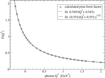
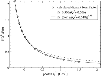
Figure 2: The pion (left) and $ud$ diquark (right) form factor, together with the fitted forms, for $\omega=0.42~{}{\rm GeV}$, $D=0.888~{}{\rm GeV}^{2}$. The analytic forms are fitted in the range $-0.3~{}{\rm GeV}^{2}<Q^{2}<1.5~{}{\rm GeV}^{2}$.

Indeed, all of the form factors do show a pole-like structure in the timelike region, see Fig. 2. For the pion, a monopole fit to the form factor

$$F(Q^{2}) = \frac{M^{2}}{Q^{2}+M^{2}}$$ (19)

using 27 calculated values of $F(Q^{2})$ with $Q^{2}$ in the range $-0.4~{}{\rm GeV}^{2}<Q^{2}<1.6~{}{\rm GeV}^{2}$ gives a mass-scale that is very close to the $\rho$ meson mass in this model, $m^{2}_{\rho}=0.55~{}{\rm GeV}^{2}$, with a $\chi^{2}$ of about 0.001. Again, these results are almost independent of the details of the interaction, as can be seen from Table 3.2.

For mesons (and diquarks) involving one strange quark and one up or down quark, one has to choose whether to attempt a monopole fit to the form factors corresponding to the individual diagrams of Fig. 1, or to the physical form factors. The neutral kaon form factor cannot be fitted by a simple monopole; however, it might be fit by a difference of two monopoles. Indeed, the vector meson dominance [VMD] mechanism suggests that one should fit the individual diagrams of Fig. 1: it is the vector meson pole in the quark-photon vertex that is at the origin of the success of VMD models. Thus, for the kaon, we have fitted $F_{u\bar{s};u}(Q^{2})$ and $F_{u\bar{s};\bar{s}}(Q^{2})$ over the same range, and the agreement with a monopole is reasonable, though not as good as for the pion; the $\chi^{2}$ value is about 0.01. Furthermore, the masses deviate somewhat more from the vector mesons $m^{2}_{\rho}=0.55~{}{\rm GeV}^{2}$ and $m^{2}_{\phi}=1.15$ GeV², see Table 3.2. As the pole positions are approached, these form factors become increasingly better represented as VMD monopoles with the $\rho$ and $\phi$ masses [16, 22].

input parameters		meson			diquark				$ud$ diquark best fit
$\omega$ $[{\rm GeV}]$	$D$ $[{\rm GeV}^{2}]$	pion	$q\bar{s};q$	$q\bar{s};q$		$ud$	$qs;q$	$qs;s$		mass	power
0.40	0.93	0.545	0.529	1.116		0.51	—	—		0.62	1.35
0.42	0.888	0.545	0.530	1.109		0.51	0.4	0.8		0.62	1.35
0.45	0.829	0.540	0.527	1.100		0.50	0.54	0.85		0.63	1.38
0.50	0.79	0.538	0.530	1.103		0.50	0.51	0.89		0.62	1.37

[] Estimates for monopole fit masses $M^{2}$ in GeV² (the flavour label $q$ stands for both $u$ and $d$ quarks).

For the diquarks, a monopole fit is not very good, as can be seen from the right panel of Fig. 2; the $\chi^{2}$ of the monopole fit is around 0.1 for the $ud$ diquark. A much better fit can be achieved by using the two-parameter fit form

$$F(Q^{2}) = \left(\frac{M^{2}}{Q^{2}+M^{2}}\right)^{a}$$ (20)

which gives a $\chi^{2}$ of 0.001. The preferred power appears to be $a=1.4$, independent of the details of the interaction. However, this does depend somewhat on the $Q^{2}$ range that is used in the fitting. Close to the $\rho$ pole in the timelike region, it does approach a pure VMD monopole form. A similar fit to the calculated pion form factor gives a power of $1.02$, which is hardly an improvement over the simple monopole fit. These fits with an arbitrary power can only be good for low and intermediate values of $Q^{2}$, since we know that asymptotically, the pseudoscalar meson and scalar diquark form factors vanish like $1/Q^{2}$.

For the $qs;q$ and $qs;s$ form factors, with $q$ standing for $u$ or $d$ quarks, the monopole masses in Table 3.2 are an estimate based on the low-$Q^{2}$ behaviour only, rather than a fit over the same range of $Q^{2}$. Complications with the analytic continuation of the quark propagator solution necessary for these calculations, and in particular the complex singularities in the quark propagator, prevent us from obtaining the form factor for these heavier states away from $Q^{2}\approx 0$.

In conclusion, we can say that simple VMD models work very well for the pion form factor, but they are less and less accurate for the heavier mesons. Nevertheless, the monopole forms for the diquarks are a reasonable approximation to these microscopic form factor calculations, and might be useful for applications in baryon calculations. An interesting consequence of these monopole fits is that the $us$ diquark form factor could potentially have a zero crossing in the spacelike region: if the mass-scale $M^{2}$ in the $F_{us;s}$ fit is more than twice as large as the mass scale $M^{2}$ in the $F_{us;u}$ fit, the “physical” form factor $\frac{2}{3}F_{us;u}(Q^{2})-\frac{1}{3}F_{us;s}(Q^{2})$ will approach zero from below for $Q^{2}\to\infty$. (In terms of VMD masses that means if $M_{\phi}^{2}>2M_{\rho}^{2}$.) However, both VMD and our current calculations indicate that this is not the case for realistic up, down, and strange quark masses.

4 Concluding remarks

The calculated charge radius of the $ud$ scalar diquark, $r_{ud}=0.71~{}{\rm fm}$, is 8% larger than the pion charge radius, $r_{\pi}=0.66~{}{\rm fm}$. This suggests that these diquarks are about 8% larger in size than pions, which agrees with the observation that the diquark BSA is about the same amount narrower in momentum space than the pion BSA [9]. These results appear to be insensitive to the details of the effective quark-quark interaction kernel, even though the actual diquark masses are sensitive to details of the interaction. Our results disagree with calculations within the Nambu–Jona-Lasinio [NJL] model [23], which suggested that the electromagnetic form factors of the pion and $ud$ scalar diquark are almost identical. Furthermore, the obtained charge radius in those NJL calculations is significantly smaller than the measured pion charge radius.

Our result for the $ud$ scalar diquark charge radius is about 20% smaller than the experimental proton charge radius, $r_{\hbox{\scriptsize proton}}=0.87~{}{\rm fm}$. If we take these radii as an indication of their physical size, it is indeed quite plausible to picture baryons as bound states of a quark and a diquark. For quantitatively reliable calculations of electromagnetic properties of nucleons however, we need not only the scalar diquark, but also the axial-vector diquark properties.

Recently, it has been suggested that pentaquarks might be composed of two diquarks (coupled together in a colour triplet) coupled to an antiquark [4]. Another possibility involving diquarks would be a (colour anti-triplet) diquark coupled to a triquark ($qq\bar{q}$) in a colour triplet state [5]. One would expect pentaquarks to be somewhat larger in size than the ordinary baryons. Based on the charge radius of the diquarks and that of the proton, we would estimate the radius of a pentaquark (in a diquark-diquark-antiquark configuration) to be $r_{\hbox{\scriptsize pentaquark}}\approx 1~{}{\rm fm}$, or about 15% larger than that of the proton.

In the timelike region, all form factors can be approximated quite well by a VMD like monopole. For increasing spacelike values of $Q^{2}$, a VMD monopole becomes less and less accurate, in particular for heavier mesons and diquarks. For moderate spacelike values of $Q^{2}$, the $ud$ diquark form factor may be interpolated by $[M^{2}/(Q^{2}+M^{2})]^{1.4}$, with a mass of about $M\approx 0.79~{}{\rm GeV}$. Asymptotically however, we expect this form factor to vanish like $1/Q^{2}$, just like the pion form factor.

I would like to thank Arne Hoell, Andreas Krassnigg, Craig Roberts, Eric Swanson, and Peter Tandy for useful discussions. Part of the computations were performed on the National Science Foundation Terascale Computing System at the Pittsburgh Supercomputing Center.

References

- [1] H. Asami, N. Ishii, W. Bentz and K. Yazaki, Phys. Rev. C 51, 3388 (1995); H. Mineo, W. Bentz and K. Yazaki, Phys. Rev. C 60, 065201 (1999) [arXiv:nucl-th/9907043]; H. Mineo, W. Bentz, N. Ishii and K. Yazaki, Nucl. Phys. A 703, 785 (2002) [arXiv:nucl-th/0201082].
- [2] M. Oettel, G. Hellstern, R. Alkofer and H. Reinhardt, Phys. Rev. C 58, 2459 (1998) [arXiv:nucl-th/9805054]; M. Oettel, L. Von Smekal and R. Alkofer, Comput. Phys. Commun. 144, 63 (2002) [arXiv:hep-ph/0109285]; R. Alkofer and M. Oettel, arXiv:hep-ph/0105320.
- [3] J. C. Bloch, C. D. Roberts, S. M. Schmidt, A. Bender and M. R. Frank, Phys. Rev. C 60, 062201 (1999) [arXiv:nucl-th/9907120]; J. C. Bloch, C. D. Roberts and S. M. Schmidt, Phys. Rev. C 61, 065207 (2000) [arXiv:nucl-th/9911068]; M. B. Hecht, M. Oettel, C. D. Roberts, S. M. Schmidt, P. C. Tandy and A. W. Thomas, Phys. Rev. C 65, 055204 (2002) [arXiv:nucl-th/0201084].
- [4] R. L. Jaffe and F. Wilczek, Phys. Rev. Lett. 91, 232003 (2003) [arXiv:hep-ph/0307341].
- [5] M. Karliner and H. J. Lipkin, Phys. Lett. B 575, 249 (2003) [arXiv:hep-ph/0402260].
- [6] M. Hess, F. Karsch, E. Laermann and I. Wetzorke, Phys. Rev. D 58, 111502 (1998) [arXiv:hep-lat/9804023].
- [7] R. T. Cahill, C. D. Roberts and J. Praschifka, Phys. Rev. D 36, 2804 (1987).
- [8] C. J. Burden, L. Qian, C. D. Roberts, P. C. Tandy and M. J. Thomson, Phys. Rev. C 55, 2649 (1997) [arXiv:nucl-th/9605027].
- [9] P. Maris, Few Body Syst. 32, 41 (2002) [arXiv:nucl-th/0204020].
- [10] C. D. Roberts and A. G. Williams, Prog. Part. Nucl. Phys. 33, 477 (1994) [arXiv:hep-ph/9403224].
- [11] C. D. Roberts and S. M. Schmidt, Prog. Part. Nucl. Phys. 45S1, 1 (2000) [arXiv:nucl-th/0005064].
- [12] R. Alkofer and L. von Smekal, Phys. Rept. 353, 281 (2001) [arXiv:hep-ph/0007355];
- [13] P. Maris and C. D. Roberts, Int. J. Mod. Phys. E 12, 297 (2003) [arXiv:nucl-th/0301049].
- [14] P. Maris and C. D. Roberts, Phys. Rev. C 56, 3369 (1997) [arXiv:nucl-th/9708029].
- [15] P. Maris and P. C. Tandy, Phys. Rev. C 60, 055214 (1999) [arXiv:nucl-th/9905056].
- [16] P. Maris and P. C. Tandy, Phys. Rev. C 61, 045202 (2000) [arXiv:nucl-th/9910033]; P. Maris and P. C. Tandy, Phys. Rev. C 62, 055204 (2000) [arXiv:nucl-th/0005015].
- [17] C. D. Roberts, Nucl. Phys. A 605, 475 (1996) [arXiv:hep-ph/9408233].
- [18] A. Holl, A. Krassnigg and C. D. Roberts, arXiv:nucl-th/0406030.
- [19] R. Fukuda and T. Kugo, Nucl. Phys. B 117, 250 (1976); D. Atkinson and D. W. Blatt, Nucl. Phys. B 151, 342 (1979); S. J. Stainsby and R. T. Cahill, Phys. Lett. A 146, 467 (1990); P. Maris and H. A. Holties, Int. J. Mod. Phys. A 7, 5369 (1992).
- [20] R. Alkofer, W. Detmold, C. S. Fischer and P. Maris, Phys. Rev. D 70, 014014 (2004) [arXiv:hep-ph/0309077].
- [21] A. Krassnigg, private communication, 2004.
- [22] D. Jarecke, P. Maris and P. C. Tandy, Phys. Rev. C 67, 035202 (2003) [arXiv:nucl-th/0208019].
- [23] C. Weiss, A. Buck, R. Alkofer and H. Reinhardt, Phys. Lett. B 312, 6 (1993) [arXiv:hep-ph/9305215].