Further explorations of Skyrme-Hartree-Fock-Bogoliubov mass formulas.
III: Role of particle-number projection

Abstract

Starting from HFB-6, we have constructed a new mass table, referred to as HFB-8, including all the 9200 nuclei lying between the two drip lines over the range of $Z$ and $N\geq 8$ and $Z\leq 120$. It differs from HFB-6 in that the wave function is projected on the exact particle number. Like HFB-6, the isoscalar effective mass $M_{s}^{*}$ is constrained to the value $0.80M$ and the pairing is density independent. The rms errors of the mass-data fit is 0.635 MeV, i.e. better than almost all our previous HFB mass formulas. The extrapolations of this new mass formula out to the drip lines do not differ significantly from the previous HFB-6 mass formula.

I Introduction

In the last few years we have been able to construct complete mass tables by the Hartree-Fock-Bogoliubov (HFB) method Samyn et al. (2002); Goriely et al. (2002); Samyn et al. (2003); Goriely et al. (2003), with the parameters of the underlying forces being fitted to essentially all of the available mass data. This paper is the third in a series of studies of possible refinements and modifications to our HFB-2 mass formula Goriely et al. (2002), the first of our models that was able to give a satisfactory fit to the new data that had accumulated since the 1995 Atomic Mass Evaluation Audi and Wapstra (1995). The most obvious reason for making such changes would be to improve the data fit, but there is also a considerable astrophysical interest in being able to generate different mass formulas even if no significant improvement in the data fit is obtained. The main point here is that the r-process of stellar nucleosynthesis proceeds through the formation of nuclei that are so highly neutron rich that their properties cannot be measured but must be inferred by extrapolating the properties of known nuclei, and there is no guarantee that mass formulas giving equivalent mass-data fits will still give the same masses out towards the neutron drip line. Moreover, even if they do, it is still possible that the underlying model (forces) will give different results for other properties relevant to the r-process (see Section 1 of the first paper of this series Samyn et al. (2003), referred to here as paper I). Predictions for the equation of state of neutron star matter could likewise differ.

In paper I Samyn et al. (2003) we discussed the role of a possible density dependence of the pairing interaction, while in paper II Goriely et al. (2003) we examined the question of the effective nucleon mass to be imposed on the Skyrme force. In the present paper we extend our HFB model by the restoration of the particle-number symmetry. In Section II we will recall the main features of the earlier HFB models relevant for the present study. In Sect. III we present our formalism for particle-number restoration. In Section IV we describe a new fit of the force parameters to the mass data, with the resulting parameter set being labelled BSk8, and discuss its ability to predict masses and radii. A complete new mass table, HFB-8, is constructed and compared with the earlier HFB-6 mass table in Sect. V. Conclusions are drawn in Sect. VI.

II Summary of the model

For convenience we recall some of the essential features of these HFB models. They are are based on conventional Skyrme forces of the form

$$v_{ij}^{ph} = t_{0}(1+x_{0}P_{\sigma})\delta({{\bf r}_{ij}})$$ (1)

$$+ t_{1}(1+x_{1}P_{\sigma})\frac{1}{2\hbar^{2}}\{p_{ij}^{2}\delta({{\bf r}_{ij}})+h.c.\}$$

$$+ t_{2}(1+x_{2}P_{\sigma})\frac{1}{\hbar^{2}}{\bf p}_{ij}.\delta({\bf r}_{ij}){\bf p}_{ij}$$

$$+ \frac{1}{6}t_{3}(1+x_{3}P_{\sigma})\rho^{\gamma}\delta({\bf r}_{ij})$$

$$+ \frac{i}{\hbar^{2}}W_{0}(\mbox{\boldmath$\sigma_{i}+\sigma_{j}$}){\bf.p}_{ij}\times\delta({\bf r}_{ij}){\bf p}_{ij}$$

in the particle-hole (ph) channel, and in the particle-particle (pp) channel a $\delta$-function pairing force acting between like nucleons treated in the full Bogoliubov framework

$$v_{ij}^{pp}=V_{\pi q}~{}\left[1-\eta\left(\frac{\rho}{\rho_{0}}\right)^{\alpha}\right]~{}\delta(\mbox{\boldmath$r$}_{ij})\ ,$$ (2)

where $\rho\equiv\rho({\bf r})$ is the local density, and $\rho_{0}$ is its equilibrium value in symmetric infinite nuclear matter (INM). Actually, it was only with models HFB-3 Samyn et al. (2003), HFB-5 Goriely et al. (2003), and HFB-7 Goriely et al. (2003) that the possibility of a density dependence in the pairing force was admitted; in all our other HFB models, HFB-1 Samyn et al. (2002), HFB-2 Goriely et al. (2002), HFB-4 Goriely et al. (2003), and HFB-6 Goriely et al. (2003) we had $\eta$ = 0, as will be the case in the present paper.

An important aspect relating to $\delta$-function pairing forces concerns the cutoff to be applied to the space of single-particle (s.p.) states over which the force is allowed to act: both BCS and Bogoliubov calculations diverge if this space is not truncated Bulgac (2002); Bulgac and Yu (2002). However, making such a cutoff is not simply a computational device but is rather a vital part of the physics, pairing being essentially a finite-range phenomenon. To represent such an interaction by a $\delta$-function force is thus legitimate only to the extent that all high-lying excitations are suppressed, although how exactly the truncation of the pairing space should be made will depend on the precise nature of the real, finite-range pairing force. It was precisely our ignorance on this latter point that allowed us in Ref. Goriely et al. (2002) to exploit the cutoff as a new degree of freedom: we found there an optimal mass fit with the spectrum of s.p. states $\varepsilon_{i}$ confined to lie in the range

$$E_{F}-\varepsilon_{\Lambda}\leq\varepsilon_{i}\leq E_{F}+\varepsilon_{\Lambda},$$ (3)

where $E_{F}$ is the Fermi energy of the nucleus in question, and $\varepsilon_{\Lambda}$ is a free parameter. We shall adopt the same parametrization in the present paper.

The mean-field states for even and odd particle number have different structure. While they are HFB states for even particle number, they are one-quasiparticle excitations for odd particle number

$$|\text{MF}\rangle = |\text{HFB}\rangle\qquad\text{even particle number,}$$ (4)

$$|\text{MF}\rangle = \hat{a}^{\dagger}_{b}|\text{HFB}\rangle\qquad\text{odd particle number.}$$ (5)

Throughout this paper, we use the canonical basis to represent the HFB states. The blocking of the unpaired particle is not calculated completely self-consistently. Doing so requires breaking the time-reversal and axial symmetries, and adding extra fields to the Hamiltonian. This is still too costly for a large-scale mass fit as performed here. Therefore we use an approximation, where the pairing correlations in odd nuclei are determined by removing the last nucleon Samyn et al. (2002). The occupation probability of the last occupied level is later corrected by adding the occupation contribution of the unpaired nucleon. The last nucleon therefore does not contribute to the pairing (it does through the pairing tensor in the spherical configuration), and the corresponding level should be treated accordingly. For the unprojected mean-field states, the occupation probability of the last occupied level $k$ is

$$w_{k}^{2}=\frac{(d(k)-2)v_{k}^{2}+1}{d(k)}\ ,$$ (6)

where the degeneracy $d(k)$ equals 2 for deformed nuclei and $2j+1$ for spherical ones ($j$ being the angular momentum quantum number); $v_{k}^{2}$ is the occupation probability obtained from the HFB equations for the level $k$ without the blocked nucleon. To compensate for the approximations done for odd particle number, we incorporate what is missing into the effective interaction and shall allow the pairing-strength parameter $V_{\pi q}$ to be different for an odd particle number ($V_{{\pi q}}^{-}$) than for an even particle number ($V_{{\pi q}}^{+}$). For example, the pairing force between neutrons depends on whether $N$ is even or odd. We also allow the pairing-strength $V_{\pi q}$ to be different for protons and neutrons, as in all our previous mass models. Another feature of the HFB-2 model Goriely et al. (2002) that we retain here is to add to the energy calculated by the HFB model a phenomenological Wigner term of the form

$$E_{W} = V_{W}\exp\Bigg{\{}-\lambda\Bigg{(}\frac{N-Z}{A}\Bigg{)}^{2}\Bigg{\}}$$ (7)

$$+ V_{W}^{\prime}|N-Z|\exp\Bigg{\{}-\Bigg{(}\frac{A}{A_{0}}\Bigg{)}^{2}\Bigg{\}}~{}.$$

The method used to solve the HFB equations for Skyrme interactions has been presented earlier in Ref. Samyn et al. (2002).

III Restoration of the particle-number symmetry

Mean-field approaches, such as the HFB used here, establish an intrinsic frame of the nucleus and consequently break several symmetries of the Hamiltonian and the wave function in the laboratory frame Ring and Schuck (1980); Bender et al. (2003). In particular, finite nuclei break translational invariance, deformed nuclei rotational invariance, reflection asymmetric shapes the parity symmetry, and the HFB framework the particle-number symmetry. These symmetry breakings are required to include the desired correlations to the modeling (as multi-particle-multi-hole states), but at the same time gives rise to an admixture of excited states to the calculated ground state. The broken symmetries can be restored rigorously by projecting the wave function on the exact quantum numbers. A simpler procedure aims at estimating the contribution to the binding energy in a suitable approximation, and to add the resulting correction to the binding energy. We adopted such a procedure in some of our previous mass formulas, in particular to estimate the center-of-mass (cm) correction from the recoil energy, and the rotational correction within the cranking model Tondeur et al. (2000). As far as the cm correction is concerned, the approximate prescription of Butler et al. Butler et al. (1984) was replaced in Goriely et al. (2003) by a more fundamental calculation of the the recoil energy. However, so far no attempt to restore the particle-number symmetry has been undertaken in any of our HFB calculations related to global mass fit. The present paper is devoted to the projection of the wave function on the exact number of particles after a variation that includes the approximate Lipkin-Nogami projection before variation (referred to as PLN), and its impact on the mass fit.

The pair correlations included in the mean-field HFB wave function $|\text{MF}\rangle$ are known to break the particle-number symmetry, as an HFB state is not an eigenstate of the particle-number operator. While the expectation value of the particle number $\langle\text{MF}|\hat{N}|\text{MF}\rangle$ is constrained to have the desired number $N$ of nucleons on the average via a Lagrange multiplier (the chemical potential), its dispersion

$$\langle\text{MF}|(\Delta\hat{N})^{2}|\text{MF}\rangle = \langle\text{MF}|\hat{N}^{2}|\text{MF}\rangle-\langle\text{MF}|\hat{N}|\text{MF}\rangle^{2}$$ (8)

$$= 2\sum_{k\lessgtr 0}u_{k}^{2}v_{k}^{2},$$

never vanishes in the presence of pairing. We use the standard notation, where $v_{k}^{2}=1-u_{k}^{2}$ is the occupation probability of the level $k$.

The particle-number symmetry is restored by applying a particle-number projection operator $\hat{P}^{N}$ on the mean-field state Ring and Schuck (1980); Heenen et al. (1993); Anguiano et al. (2001, 2002)

$$|\Phi\rangle=\frac{\hat{P}^{N}|\text{MF}\rangle}{\langle\text{MF}|\hat{P}^{N}|\text{MF}\rangle^{1/2}}$$ (9)

which eliminates all components of the HFB state with a particle number different from $N$. $|\Phi\rangle$ is a normalized eigenstate of the particle-number operator. The particle-number projector is given by

$$\hat{P}^{N}=\frac{1}{2\pi}\int_{0}^{2\pi}d\phi\ \,e^{i\phi(\hat{N}-N)}.$$ (10)

The integration interval of the gauge angle $\phi$ can be reduced to $[0,\pi]$ for intrinsic wave functions with a well-defined “number parity” quantum number, i.e.,  for even-even systems as well as odd systems if treated in the blocking approximation (see below). For practical applications, the integral over the gauge angle in the particle-number projection operator has to be discretized,

$$P_{n}(M_{g})=\frac{1}{M_{g}}\sum_{m=1}^{M_{g}}e^{i\phi_{m}(\hat{N}-n)}.$$ (11)

We use the Fomenko prescription Fomenko (1970), where $\phi_{m}=\pi(m-1)/M_{g}$ and $M_{g}$ is the number of angles in the interval $[0,\pi]$ used in the calculation. It can be shown that this particular choice of the projector removes all unwanted contaminations of the states up to $n\pm 2M_{g}$ Ring and Schuck (1980). In order to avoid certain numerical problems that arise at $\phi=\frac{\pi}{2}$ when $v^{2}_{k}$ has accidentally the value $0.5$ Anguiano et al. (2001) we restrict ourselves to odd values of $M_{g}$, choosing finally $M_{g}=11$ for both protons and neutrons in all calculations. The particle number dispersion is subsequently checked to verify that the projection actually worked.

The particle-number symmetry restoration is performed in two steps. First, an approximate projection before variation is performed within the Lipkin-Nogami prescription Nogami (1973); Pradhan et al. (1973); Reinhard et al. (1996); Flocard and Onishi (1997); Anguiano et al. (2001), where we take only the pairing part of the interaction into account when calculating $\lambda_{2}$. In a second step, the converged HFB states are then exactly projected as described by Eq. (10). As usually done, we constrain the HFB states to the same particle number that we project out exactly afterwards. In such a projection after variation approach, the main task for the Lipkin-Nogami scheme is to enforce the presence of pair correlations in the HFB states for all $N$ and $Z$ and all deformations to avoid the breakdown of pairing for small level densities. This two-step approach was shown to be an excellent approximation to the exact self-consistent particle-number projection before variation Anguiano et al. (2002).

The nuclear mass and all other observables are calculated from the projected state applying a generalized Wick’s theorem. The basic contractions needed for that are given by Anguiano et al. (2001)

$$\rho_{kk^{\prime}}(\phi) \equiv \frac{\langle\text{MF}|a^{{\dagger}}_{k}a_{k^{\prime}}e^{i\phi\hat{N}}|\text{MF}\rangle}{\langle\text{MF}|\text{MF}(\phi)\rangle}$$ (12)

$$= \frac{v^{2}_{k}e^{2i\phi}}{u^{2}_{k}+v^{2}_{k}e^{2i\phi}}\delta_{kk^{\prime}}=\rho_{\bar{k}\bar{k}^{\prime}}(\phi)\ ,$$

$$\kappa_{k\bar{k}^{\prime}}(\phi) \equiv \frac{\langle\text{MF}|a^{{\dagger}}_{k}a^{{\dagger}}_{\bar{k}^{\prime}}e^{i\phi\hat{N}}|\text{MF}\rangle}{\langle\text{MF}|\text{MF}(\phi)\rangle}$$ (13)

$$= \frac{-u_{k}v_{k}}{u^{2}_{k}+v^{2}_{k}e^{2i\phi}}\delta_{kk^{\prime}}=-\kappa_{\bar{k}k^{\prime}}(\phi)\ ,$$

$$\tilde{\kappa}_{k\bar{k}^{\prime}}(\phi) \equiv \frac{\langle\text{MF}|a_{k}a_{\bar{k}^{\prime}}e^{i\phi\hat{N}}|\text{MF}\rangle}{\langle\text{MF}|\text{MF}(\phi)\rangle}$$ (14)

$$= \frac{u_{k}v_{k}e^{2i\phi}}{u^{2}_{k}+v^{2}_{k}e^{2i\phi}}\delta_{kk^{\prime}}=-\tilde{\kappa}_{\bar{k}k^{\prime}}(\phi),$$

where we introduced the shorthand notation $|\text{MF}(\phi)\rangle\equiv e^{i\phi\hat{N}}|\text{MF}\rangle$ for a MF state rotated in gauge space. We employ the phase convention ($u_{\bar{k}},v_{\bar{k}})=(u_{k},-v_{k})$, where $k$ denotes single-particle states with positive angular momentum projection on the symmetry axis, and $\bar{k}$ the corresponding time-reversed states with negative angular momentum projection on the symmetry axis. For the blocked orbital in a mean-field state with odd particle number, the contractions of the level $k$ are determined by removing the blocked nucleon, since it should not enter the particle number projection. Of course, the contribution of this unpaired nucleon is added to Eq. (12) afterwards (see, for instance, Eq. (23)). In order to express the expectation value of observables in the projected state, it is useful to introduce normalized $\phi$-dependent overlaps

$$O(\phi,n)\equiv\frac{\langle\text{MF}|\text{MF}(\phi)\rangle\,e^{-in\phi}}{\sum_{m=1}^{M_{g}}\langle\text{MF}|\text{MF}(\phi_{m})\rangle\,e^{-in\phi_{m}}}\ .$$ (15)

Based on Eq. (12), the number of particles of the projected state can then be written as

$$\langle\Phi|\hat{N}|\Phi\rangle=\sum_{m=1}^{M_{g}}O(\phi_{m},n)\;{\rm Tr}[\rho(\phi_{m})]\ ,$$ (16)

which reduces to the familiar $\langle\hat{N}\rangle=2\sum_{k>0}v_{k}^{2}$ if $M_{g}=1$.

The particle-number projected energy depends on the $\phi$-dependent generalized densities and is calculated by an integration over the spatial coordinates ${\bf r}$ and the summation over the two sets of gauge angles $\phi^{q}_{m}$ ($q=n,p$). The total mean-field energy can therefore be expressed as

$$E_{\text{mf}} = \sum_{m_{n}=1}^{M_{g}}\sum_{m_{p}=1}^{M_{g}}O(\phi^{n}_{m_{n}},n)\,O(\phi^{p}_{m_{p}},p)$$ (17)

$$\times\int\mathrm{d}{\bf r}\;{\cal E}_{\text{mf}}({\bf r},\phi^{n}_{m_{n}},\phi^{p}_{m_{p}}),$$

where ${\cal E}_{\text{mf}}$ is the Skyrme energy density functional (obtained with Eq. (3a) of Tondeur et al. (2000) and the $\phi-$dependent densities). The pairing energy is calculated similarly:

$$E_{\text{pair},q} = \sum_{m_{n}=1}^{M_{g}}\sum_{m_{p}=1}^{M_{g}}O(\phi^{n}_{m_{n}},n)\,O(\phi^{p}_{m_{p}},p)$$ (18)

$$\times\int\mathrm{d}{\bf r}\;{\cal E}_{\text{pair},q}({\bf r},\phi^{n}_{m_{n}},\phi^{p}_{m_{p}}),$$

where

$${\cal E}_{\text{pair},q}({\bf r},\phi^{q}_{m_{q}},\phi^{q}_{m_{q}}) = V_{\pi q}{\rm Tr}[\kappa(\phi^{q})]{\rm Tr}[\tilde{\kappa}(\phi^{q})]$$ (19)

$$\times\left(1-\eta\bigg{[}\frac{(\rho({\bf r},\phi^{n}_{m_{n}},\phi^{p}_{m_{p}})}{\rho_{0}}\bigg{]}^{\alpha}\right).$$

For the density-dependence in $E_{\text{mf}}$ and $E_{\text{pair}}$ we choose the mixed density obtained from Eq. (12), as done in most applications involving the mixing of different mean-field states. This choice, however, is not unique, see the discusion in Refs. Anguiano et al. (2001); Rodriguez-Guzman et al. (2002) and references given therein.

III.0.1 Decomposition of mean-field states

The weight of the $n^{\prime}$-nucleon wave function in the decomposition of the unprojected $n$-particle HFB state $|\text{MF}_{n}\rangle$ in given by the overlap

$${\cal O}_{n^{\prime}} = \langle\text{MF}_{n}|\hat{P}^{n^{\prime}}|\text{MF}_{n}\rangle.$$ (20)

This quantity can be used to illustrate the particle number dispersion of the HFB states.

An example is given in Fig. 1 for ²⁴⁰Pu, where we compare the spherical configuration with the deformed equilibrium one, which has a quadrupole moment of $Q=2782$ fm². The decomposition is significantly different. In lowest order, the distribution of the weights has a Gaussian shape Flocard and Onishi (1997)

$${\cal O}_{n^{\prime}}\simeq\frac{2}{\sqrt{2\pi\sigma^{2}}}\exp\Big{(}-\frac{(\langle\text{MF}|\hat{N}|\text{MF}\rangle-n^{\prime})^{2}}{2\sigma^{2}}\Big{)},$$ (21)

where the width of the Gaussian $\sigma^{2}=\langle\text{MF}|(\Delta\hat{N})^{2}|\text{MF}\rangle$ is determined by the particle-number dispersion of the unprojected state, Eq. (8). In the specific case of ²⁴⁰Pu, the Gaussian is more spread for the spherical shape, where pairing is stronger due to the larger level density around the Fermi surface.

Figure 1: Proton (left) and neutron (right) overlaps between the unprojected HFB wave function of ²⁴⁰Pu and its state projected on $n^{\prime}$ ($N$ or $Z$) nucleons; diamonds refer to spherical overlaps, crosses to deformed ones; the full line corresponds to a Gaussian centered on $n=94$ (protons) or 146 (neutrons) and of standard deviation $\sigma^{2}$ equal to the particle-number dispersion.

The different blocking prescription in spherical and deformed configurations leads to significant variations in the weight of neighbouring nuclei in the wave function, as seen in Fig. 2 for the spherical ⁹⁹In and ¹⁰⁰In isotopes: the blocked nucleon in the spherical case is not removed from a doubly-degenerate level (to leave it empty) but removed from the $g_{9/2}$ level, which is equivalent to the removal of 20$\%$ of a nucleon on the last five doubly-degenerate levels of a deformed configuration. The weight of the wave functions of adjacent nuclei is therefore higher (in the $Z=49$ or $N=51$ In isotopes) if the spherical code is used. It is also observed that the deviation between Eq. (21) and Eq. (20) is more pronounced, due to a shell closure effect.

Figure 2: Same as Fig. 1 for the spherical ⁹⁹In and ¹⁰⁰In istopes. The Gaussian approximation, Eq. 21 (thin line with dots or dashes obtained from the spherical or deformed code) cannot describe the pronounced shell closure. For $Z=49$ or $N=51$, the overlaps obtained with the deformed code differ significantly from the overlaps calculated assuming spherical symmetry, due to a different implementation of the blocking approximation.

For consistency, the cm correction should be calculated from the particle-number projected state. Written concisely, the gauge angle-dependent cm energy of the particle-number projected state reads

$${\mathcal{E}}_{cm}(\phi) = -\frac{\hbar^{2}}{2M}\Big{[}2\sum_{k>0}\rho_{kk}\Delta_{kk}+2\sum_{k,l>0}(\rho_{kk}\rho_{ll}+\kappa_{k\bar{k}}\tilde{\kappa}_{l\bar{l}})$$ (22)

$$\qquad(\mbox{\boldmath$\nabla$}_{kl}\cdot\mbox{\boldmath$\nabla$}^{*}_{kl}+\mbox{\boldmath$\nabla$}_{k\bar{l}}\cdot\mbox{\boldmath$\nabla$}^{*}_{k\bar{l}})\Big{]}.$$

For odd nuclei, $(\rho_{kk}\rho_{ll}+\kappa_{k\bar{k}}\tilde{\kappa}_{l\bar{l}})$ becomes

$$\Big{[}\frac{(d(k)-2\delta_{b}(k))\rho_{kk}+\delta_{b}(k)}{d(k)}\$$ (23)

$$\frac{(d(l)-2\delta_{b}(l))\rho_{ll}+\delta_{b}(l)}{d(l)}+\kappa_{k\bar{k}}\tilde{\kappa}_{l\bar{l}}\Big{]}\quad,$$

with $\delta_{b}(k)=1$ if the blocked nucleon is on the level $k$ (0 otherwize). The cm energy (for one nucleon species $q$) is then

$$E_{cm,q}=\sum_{m=1}^{M_{g}}O(\phi_{m},q)\,{\mathcal{E}}_{cm,q}({\bf r},\phi_{m}).$$ (24)

Finally, note that as far as the rotational correction is concerned, we will restrict ourselves to the simplified cranking formula, although ideally the rotational symmetry should also be restored with projection techniques. So far, in all our global mass fits, we adopted the rotational correction calculated from the HFB states

$$E_{\text{rot}}=\frac{\langle\text{MF}|\hat{J}^{2}|\text{MF}\rangle}{2{\mathcal{I}}}\ ,$$ (25)

where $\hat{J}$ is the total angular momentum operator in the intrinsic frame and ${\mathcal{I}}$ the moment of inertia. The cranking model Inglis (1954, 1956); Belyaev (1961) gives this latter quantity as

$${\mathcal{I}}_{cr} = 2\sum_{k,k^{\prime}>0}\frac{|\langle k|J_{x}|k^{\prime}\rangle|^{2}}{E_{k}+E_{k^{\prime}}}(u_{k}v_{k^{\prime}}-u_{k^{\prime}}v_{k})^{2},$$ (26)

where the summation runs over quasi-particle s.p. states, the $E_{k}$ are the corresponding quasi-particle energies, the matrix elements are calculated in the canonical basis, and $v_{k}^{2}=1-u_{k}^{2}$ are the corresponding occupation probabilities.

While the cranking model is in general quite satisfactory, a major problem in our mass-model applications arises from the fact that a priori we do not know which nuclei will be spherical (or quasi-spherical), for which nuclei a numerical problem arises from the 0/0 indeterminacy in Eq. (25); $E_{rot}$ must vanish, of course, for spherical nuclei. A way around this problem, introduced in Ref. Pearson et al. (1991), is to take for the ${\mathcal{I}}$ the linear combination

$${\mathcal{I}}_{mix}=a{\mathcal{I}}_{cr}+(1-a){\mathcal{I}}_{rig}\quad,$$ (27)

where ${\mathcal{I}}_{rig}$ is the rigid-body moment of inertia

$${\mathcal{I}}_{rig} = \frac{M}{3}(2R^{2}A+\frac{1}{2}Q)\quad,$$ (28)

in which $R$ is the rms matter radius of the nucleus, $M$ the nucleon mass, and $Q$ the quadrupole moment. The value of $a$ was originally taken to be 0.8, but was reduced to 0.75 in Ref. Goriely et al. (2001) and kept unchanged in all subsequent mass formulas (HFB-1–HFB-7). However, we see from Table 1 that with this prescription the deformation energies ${\Delta}E_{iso}$ of highly deformed shape isomers, i.e., their energy relative to the ground state of the nucleus in question, are badly underestimated, and can even be negative. For this reason we adopt for the rotational energy the phenomenological prescription

$$E_{rot}=bE_{rot}^{crank}~{}\tanh(c|\beta_{2}|)\ ,$$ (29)

or equivalently introduce a new prescription based on the cranking value of the moment of inertia modified as follows:

$${\mathcal{I}}_{crth} = \frac{1}{b}{\mathcal{I}}_{cr}\coth(c|\beta_{2}|).$$ (30)

Here, the dimensionless quadrupole moment $\beta_{2}$ is defined as a function of the quadrupole moment $Q_{2}$ and the reduced radius $R_{0}$ by $\beta_{2}=\sqrt{5\pi}Q_{2}/(3AR_{0}^{2})$. Experimental information on the mass of well deformed nuclei, but also the energy of the shape isomers in the actinide region is used to determine the free parameters $(b,c)$. Values of $(b,c)$ range from (0.6,5.5) to (0.7,3.5). For HFB-8, we adopt $b=0.65$ and $c=4.5$. We find that this prescription not only is equivalent to the “mixed” prescription (27) for ground states, i.e., for masses, and likewise avoids any problems in the spherical limit, but also leads to considerable improvements in the estimates for the shape isomers, as can be seen from the penultimate column of Table 1.

Table 1: Comparison between experimental Bjørnholm and Lynn (1980); Blons et al. (1988); jae (1996); Hunyadi et al. (2001) and theoretical (reflection symmetric assumed) energies of shape isomers obtained with the HFB+PLN(BSk8) model using three different rotational correction prescriptions: Eq. (30) (modified cranking), Eq. (27) (mix with $a=0.87$), and Eq. (28) (rigid). The last two lines show the rms and mean deviations, respectively, compared to experiment. All quantities in MeV.

Z	N	A	exp	crth	mix	rig
90	140	230	2.25	2.6	1.6	2.2
	141	231	2.3	2.4	1.3	2.1
	143	233	2.3	2.5	1.5	2.3
92	143	235	2.5	2.3	1.2	1.9
	144	236	2.3	2.3	1.2	1.8
	145	237	2.2	2.2	0.9	1.9
	146	238	2.6	2.4	1.4	2.0
	147	239	1.9	1.9	0.6	1.5
93	144	237	2.7	1.7	0.7	1.3
	145	238	2.3	1.6	0.6	1.4
94	141	235	2.6	1.5	0.4	1.1
	143	237	2.3	1.9	0.8	1.4
	144	238	2.4	1.8	0.7	1.3
	145	239	2.2	1.8	0.6	1.3
	146	240	2.25	1.9	0.8	1.5
	147	241	1.9	1.3	0.1	0.9
	149	243	1.7	2.0	0.8	1.6
	150	244	2.0	2.2	1.0	1.7
95	144	239	2.4	1.4	0.4	1.0
	145	240	2.6	1.4	0.4	1.1
	146	241	2.2	1.7	0.6	1.3
	147	242	2.3	1.0	-0.2	0.6
	148	243	2.0	1.7	0.6	1.3
	149	244	1.6	1.6	0.5	1.3
96	145	241	2.0	1.1	0.0	0.7
	146	242	1.8	1.3	0.2	0.8
	147	243	1.5	1.1	-0.2	0.6
	148	244	1.04	1.5	0.3	1.0
	149	245	1.7	1.3	0.0	0.9
97	147	244	2.0	0.6	-1.0	0.1
$\sigma$				0.64	1.62	0.95
$\epsilon$				0.40	1.54	0.80

The rotational correction should be accompanied by corrections for vibrational zero-point motion. To the best of our knowledge, there exists no strategy to estimate them properly and at the same time include them in a global mass fit as ours with current computing resources. Common strategies are to calculate RPA correlations Stetcu and Johnson (2002); Baroni et al. , usually restricted to spherical nuclei, or to use the generator coordinate method Bender et al. (2004). More research in this direction is necessary in the future.

IV The mass fit

To study the impact of the PLN framework, we start from the BSk6 force Goriely et al. (2003), keeping some of its characteristics: an isoscalar effective mass $M^{*}_{s}/M$ constrained to 0.8, the symmetry energy $J$ to 28 MeV, the $\gamma$ exponent in the $t_{3}$ term of Eq.( 1) to 1/4, and a density-independent pairing interaction (i.e., $\eta=0$). The results of the HFB-8 mass fit of the new HFB+PLN model are presented in Table  2, where for comparison we also show the results of the HFB-6 model. Since the latter was fitted to the 2135 nuclei with $Z,N\geq 8$ whose masses had been measured and compiled in the unpublished 2001 Atomic Mass Evaluation (AME) of Audi and Wapstra Audi and Wapstra (2001) we show results for both this data set and the 2149 measured masses of the updated AME that was released and published at the end of 2003 Audi et al. (2003). Experimental and calculated mass excesses are compared in Fig. 3.

Table 2: Rms ($\sigma$) and mean ($\bar{\epsilon}$) errors (in MeV) in the predictions of masses $M$ obtained with the BSk6 and BSk8 forces with respect to the 2135 nuclei in the 2001 AME Audi and Wapstra (2001) and the 2149 nuclei in the 2003 AME Audi et al. (2003). The last two lines correspond to the rms and mean errors (in fm) in the predictions of the 523 measured charge radii ($r_{c}$).

	BSk6	BSk8
$\sigma(M)$ (2135 nuclei)	0.684	0.659
$\bar{\epsilon}(M)$ (2135 nuclei)	0.021	0.005
$\sigma(M)$ (2149 nuclei)	0.666	0.635
$\bar{\epsilon}(M)$ (2149 nuclei)	0.014	0.009
$\sigma(r_{c})$ (523 nuc)	0.0262	0.0250
$\bar{\epsilon}(r_{c})$ (523 nuc)	-0.0028	0.0047

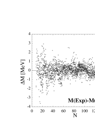
Figure 3: differences between experimental and calculated mass excesses as a function of the neutron number $N$ for the HFB-8 mass tables

The parameters of the force BSk6 and BSk8 are compared in Table 3, while the macroscopic parameters, i.e., the parameters relating to (semi-) infinite nuclear matter calculated for these forces, are shown in Table 4. These include, in addition to the previously defined parameters, $a_{v}$, the energy per nucleon at equilibrium in symmetric infinite nuclear matter, $M^{*}_{v}/M$ the ratio of the isovector effective nucleon mass at density $\rho_{0}$ to the real nucleon mass $M$, $K_{v}$, the incompressibility, $G_{0}$ and $G_{0}^{\prime}$ the Landau parameters as defined in Ref. Nguyen Van Giai and Sagawa (1981), $\rho_{frmg}$, the density at which neutron matter flips over into a ferromagnetic state that has no energy minimum and would collapse indefinitely Kutschera and Wójcik (1994), $a_{sf}$, the surface coefficient, and $Q$, the surface-stiffness coefficient Myers and Swiatecki (1969) (the meaning of $G_{0}$, $G_{0}^{\prime}$, and $\rho_{frmg}$ is critically discussed in Bender et al. (2003, 2002)).

Table 3: Skyrme-force and pairing-force parameters of BSk6 and BSk8

	BSk6	BSk8
$t_{0}$ [MeV fm3]	-2043.317	-2035.525
$t_{1}$ [MeV fm5]	382.127	398.8208
$t_{2}$ [MeV fm5]	-173.879	-196.0032
$t_{3}$ [MeV fm3+3γ]	12511.7	12433.36
$x_{0}$	0.735859	0.773828
$x_{1}$	-0.799153	-0.822006
$x_{2}$	-0.358983	-0.389640
$x_{3}$	1.234779	1.309331
$W_{0}$ [MeV fm5]	142.4	147.8
$\gamma$	1/4	1/4
$V^{+}_{n}$ [MeV fm3]	-321.2	-314.0
$V^{-}_{n}$ [MeV fm3]	-337.9	-329.8
$V^{+}_{p}$ [MeV fm3]	-324.5	-293.0
$V^{-}_{p}$ [MeV fm3]	-342.4	-309.9
$\eta$	0	0
$\alpha$	0	0
$\varepsilon_{\Lambda}$ [MeV]	17	17
$V_{W}$ [MeV]	1.76	1.85
$\lambda$	700	780
$V_{W}^{\prime}$ [MeV]	0.58	0.66
$A_{0}$	28	26
$a$ (Eq.(27))	0.75	-
$b,c$ (Eq.(29))	-	0.65,4.5

Table 4: Macroscopic parameters of the forces BSk6 and BSk8

	BSk6	BSk8
$a_{v}$ [MeV]	-15.749	-15.824
$\rho_{0}$ [fm-3]	0.1575	0.1589
$J$ [MeV]	28.0	28.0
$M^{*}_{s}/M$	0.80	0.80
$M^{*}_{v}/M$	0.86	0.87
$K_{v}$ [MeV]	229	230
$G_{0}$	0.066	0.042
$G_{0}^{{}^{\prime}}$	0.312	0.261
$\rho_{frmg}/\rho_{0}$	1.82	1.70
$a_{sf}$ [MeV]	17.18	17.64
$Q$ [MeV]	53.4	53.9

The Skyrme parameters have changed little from the original BSk6 Skyrme force; the pairing strengths have instead decreased significantly, by 2$\%$ for $V_{\pi n}$ and 11$\%$ for $V_{\pi p}$. For the first time we obtain $V_{\pi p}<V_{\pi n}$, which is what one expects when the zero-range pairing force with different coupling constants for protons and neutrons, Eq. (2), shall simulate an attractive isospin-invariant isovector pairing force and a repulsive isospin symmetry-breaking pairing force originating from the Coulomb interaction. The new Skyrme parametrization globally improves the prediction of experimental masses, as shown in Table 2. The comparison between the HFB-6 and HFB-8 mass tables, in particular towards the neutron dripline is further discussed in Sect. V.

Figure 4: Comparison of the theoretical and experimental charge radii for the 523 nuclei listed in the 1994 compilation of Nadjakov et al. (1994)

Figure 5: Comparison of the theoretical (full line) and experimental (crosses with error bars) charge densities for for ³²S and ²⁰⁸Pb. Experimental data are from Fricke et al. (1995).

Table 2 also shows the rms and mean deviations between theoretical and experimental charge radii for the 523 nuclei listed in the 1994 compilation Nadjakov et al. (1994) (for more details on the HFB derivation of the charge radii, see Buchinger et al. (2001)). The comparison is given in Fig. 4. The overall agreement with experiment is seen to be excellent, although some fine structure related to local anomalies is not reproduced in all details. Similarly, the radial charge density distribution of spherical nuclei as obtained from the charge form factor is found to be well reproduced even down to the centre of the nucleus, see the examples of ³²S and ²⁰⁸Pb given in Fig. 5. Such a good agreement between theoretical and experimental densities and radii is strongly related to the adopted value of the saturation density $\rho_{0}$ (Table III) or equivalently the Fermi momentum $k_{F}=1.33$ fm^-1 given by $(3\pi^{2}\rho_{0}/2)^{1/3}$. However, in the case of densities, the excellent agreement with experiment both in the surface and inside the nucleus must be regarded as fortuitous, being completely beyond our control in mass fits of the kind described here.

V Extrapolations

With the BSk8 Skyrme force determined as described we constructed a complete mass table, labeled HFB-8, for the same nuclei as were included in the HFB-6 tables, i.e., all the nuclei lying between the two drip lines over the range of $Z$ and $N\geq 8$ and $Z\leq 120$.

The HFB-8 masses are compared in Figs. 6-7 with the HFB-6 masses.

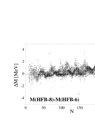
Figure 6: Differences between the HFB-8 and the HFB-6 masses as a function of the neutron number $N$ for all nuclei with $8\leq Z\leq 120$ lying between the two drip lines.

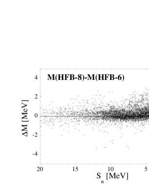
Figure 7: Differences between the HFB-8 and the HFB-6 masses as a function of the neutron separation energy $S_{n}$ for all nuclei with $8\leq Z\leq 120$ lying between the two drip lines.

Differences seldom exceed some 2 MeV, even close to the neutron dripline; the largest deviations are found for open shell nuclei. Shell effects far away from stability are found to be very similar for the two mass tables. Moreover, the HFB-8 shell gaps are very similar to the shell gaps obtained with the HFB-6 mass formula so that they are not shown here. These results once again confirm the relative stability of the HFB mass predictions with respect to different parametrizations or frameworks, as already emphasized in Goriely et al. (2003).

VI Conclusions

The pairing correlations included in the HFB wave function are known to break the particle-number symmetry. The restoration of the exact particle number is done on the basis of the projection technique, i.e by projecting the wave function on the exact number of particles after a variation that includes the approximate LN projection before variation. Doing so, we have constructed a new Skyrme force, labelled BSk8, the parameters of which reproduce the 2149 measured masses with an rms error of 0.635 MeV. The final table, referred to as HFB-8, includes all the 9200 nuclei lying between the two drip lines over the range of $Z$ and $N\geq 8$ and $Z\leq 120$. The extrapolations of this new mass formula out to the drip lines do not differ significantly from the previous HFB-6 mass formula obtained without the restoration of the particle-number symmetry.
Acknowledgements. M.S. and S.G. are FNRS Research Fellow and Associate, respectively. J.M.P. acknowledges financial support from NSERC (Canada). This work has been partly supported by Grant No. PAI-P5-07 of the Belgian Office for Scientific Policy. M.B. acknowledges financial support from the European Community.

References

- Samyn et al. (2002) M. Samyn, S. Goriely, P.-H. Heenen, J. M. Pearson, and F. Tondeur, Nucl. Phys. A700, 142 (2002).
- Goriely et al. (2002) S. Goriely, M. Samyn, P.-H. Heenen, J. M. Pearson, and F. Tondeur, Phys. Rev. C 66, 024326 (2002).
- Samyn et al. (2003) M. Samyn, S. Goriely, and J. M. Pearson, Nucl. Phys. A725, 69 (2003).
- Goriely et al. (2003) S. Goriely, M. Samyn, M. Bender, and J. M. Pearson, Phys. Rev. C 68, 054325 (2003).
- Audi and Wapstra (1995) G. Audi and A. Wapstra, Nucl. Phys. A595, 409 (1995), www-csnsm.in2p3.fr/AMDC/.
- Bulgac (2002) A. Bulgac, Phys. Rev. C 65, 051305 (2002).
- Bulgac and Yu (2002) A. Bulgac and Y. Yu, Phys. Rev. Lett. 88, 042504 (2002).
- Ring and Schuck (1980) P. Ring and P. Schuck, The Nuclear Many-Body Problem (Springer, Berlin, 1980).
- Bender et al. (2003) M. Bender, P.-H. Heenen, and P.-G. Reinhard, Rev. Mod. Phys. 75, 121 (2003).
- Tondeur et al. (2000) F. Tondeur, S. Goriely, J. M. Pearson, and M. Onsi, Phys. Rev. C 62, 024308 (2000).
- Butler et al. (1984) M. Butler, D. Sprung, and J. Martorell, Nucl. Phys. A422, 157 (1984).
- Heenen et al. (1993) P.-H. Heenen, P. Bonche, J. Dobaczewski, and H. Flocard, Nucl. Phys. A561, 367 (1993).
- Anguiano et al. (2001) M. Anguiano, J. Egido, and L. Robledo, Nucl. Phys. A696, 467 (2001).
- Anguiano et al. (2002) M. Anguiano, J. Egido, and L. Robledo, Phys. Lett. B 545, 62 (2002).
- Fomenko (1970) V. N. Fomenko, J. Phys. (London) A3, 8 (1970).
- Nogami (1973) Y. Nogami, Phys. Rev. 134, B313 (1973).
- Pradhan et al. (1973) H. Pradhan, Y. Nogami, and J. Law, nucl. Phys. A 201, 357 (1973).
- Reinhard et al. (1996) P.-G. Reinhard, W. Nazarewicz, M. Bender, and J. A. Maruhn, Phys. Rev. C 53, 2776 (1996).
- Flocard and Onishi (1997) H. Flocard and N. Onishi, Ann. Phys. 254, 275 (1997).
- Rodriguez-Guzman et al. (2002) R. Rodriguez-Guzman, J. L. Egido, and L. M. Robledo, Nucl. Phys. A709, 201 (2002).
- Inglis (1954) D. Inglis, Phys. Rev. 96, 1059 (1954).
- Inglis (1956) D. Inglis, Phys. Rev. 103, 1786 (1956).
- Belyaev (1961) S. Belyaev, Nucl. Phys. 24, 322 (1961).
- Pearson et al. (1991) J. M. Pearson, Y. Aboussir, A. K. Dutta, R. C. Nayak, M. Farine, and F. Tondeur, Nucl. Phys. A528, 1 (1991).
- Goriely et al. (2001) S. Goriely, F. Tondeur, and J. M. Pearson, At. Data Nucl. Data Tables 77, 311 (2001).
- Bjørnholm and Lynn (1980) S. Bjørnholm and J. Lynn, Rev. Mod. Phys. 52, 725 (1980).
- Blons et al. (1988) J. Blons, B. Fabbro, C. Mazur, D. Paya, and M. Ribrag, Nucl. Phys. A477, 231 (1988).
- jae (1996) Experimental total half-lifes, Japan Atomic Energy Research Institute (1996).
- Hunyadi et al. (2001) M. Hunyadi, D. Gassmann, A. Krasznahorkay, D. Habs, P. Thirolf, M. Csatlós, Y. Eisermann, T. Faestermann, G. Graw, J. Gulyás, et al., Phys. Lett. B 505, 27 (2001).
- Stetcu and Johnson (2002) I. Stetcu and C. W. Johnson, Phys. Rev. C 66, 034301 (2002).
- (31) S. Baroni, M. Armati, F. Barranco, R. A. Broglia, G. Colo’, G. Gori, and E. Vigezzi, nucl-th/0404019.
- Bender et al. (2004) M. Bender, G. Bertsch, and P.-H. Heenen, Phys. Rev. C 69, 034340 (2004).
- Audi and Wapstra (2001) G. Audi and A. Wapstra (2001), private communication.
- Audi et al. (2003) G. Audi, A. Wapstra, and C. Thibault, Nucl. Phys. A729, 3 (2003), www-csnsm.in2p3.fr/AMDC.
- Nguyen Van Giai and Sagawa (1981) Nguyen Van Giai and H. Sagawa, Phys. Lett. B 106, 379 (1981).
- Kutschera and Wójcik (1994) M. Kutschera and W. Wójcik, Phys. Lett. B 325, 271 (1994).
- Myers and Swiatecki (1969) W. D. Myers and W. J. Swiatecki, Ann. Phys. 55, 395 (1969).
- Bender et al. (2002) M. Bender, J. Dobaczewski, J. Engel, and W. Nazarewicz, Phys. Rev. C 65, 054322 (2002).
- Nadjakov et al. (1994) E. Nadjakov, K. Marinova, and Y. Gangrsky, At Data Nucl. Data Tables 56, 133 (1994).
- Fricke et al. (1995) G. Fricke, C. Bernhardt, K. Heilig, L. Schaller, L. Shellenberger, E. Shera, and C. de Jager, At. Data Nucl. Data Tables 60, 177 (1995).
- Buchinger et al. (2001) F. Buchinger, J. M. Pearson, and S. Goriely, Phys. Rev. C 64, 067303 (2001).