Relativistic Hartree approach with exact treatment of vacuum polarization for finite nuclei

Abstract

We study the relativistic Hartree approach with the exact treatment of the vacuum polarization in the Walecka ($\sigma-\omega$) model. The contribution from the vacuum polarization of nucleon-antinucleon field to the source term of the meson fields is evaluated by performing the energy integrals of the Dirac Green function along the imaginary axis. With the present method of the vacuum polarization in finite system, the total binding energies and charge radii of ¹⁶O and ⁴⁰Ca can be reproduced. On the other hand, the level-splittings in the single-particle level, in particular the spin-orbit splittings, are not described nicely because the inclusion of vacuum effect provides a large effective mass with small meson fields. We also show that the derivative expansion of the effective action which has been used to calculate the vacuum contribution for finite nuclei gives a fairly good approximation.

PACS number(s): 21.10.-k,21.60.-n, 13.75.Cs

I Introduction

It is well known that the relativistic field theory based on the hadrons referred to as quantum hadrodynamics (QHD) has been of great success in describing the ground states of finite nucleiWA74 . When the energy functional of the relativistic mean field (RMF) is fitted to nuclear saturation, the RMF model automatically produces an appropriate order of the spin-orbit splitting of nuclei, the spin-observables of the proton-nucleus scattering and energy dependence of the proton-nucleus optical potential. In RMF, however, only positive-energy nucleons are taken into account in the calculation in spite of the existence of solutions with negative energy, which is one of the interesting characters of the relativistic picture. The negative-energy states are observables in antinucleonic atom. The bound levels of antinucleonic atom are predicted to be much deeper than those of ordinary nucleon since the magnitudes of nucleon-scalar and -vector self energies, which are very large, cancel each other to provide the usual binding energy in the nucleon sector, while they add each other in the antinucleon sector (see Ref. KL02 and references therein). It is important to study if this feature remains to be the case, when we treat the negative-energy states explicitly in the QHD framework. In particular, to know how deep the antinucleons are bound in the nucleus provides valuable information for the search of the exotic collective antimatter production proposed by GreinerGR95 .

Recently, the gauge invariant nuclear-polarization calculation was carried out in the relativistic random-phase approximation (RRPA) based on the RMF theory. It was found that the RRPA eigenstates with negative energy have a significant role because the transverse form factors to these states become considerably largeHA04 . If antinucleons are deeply bound, the transverse response function has a contribution from the antinucleon states with lower energy than twice the nucleon mass. Then, electron-scattering or photo-absorption may confirm the large binding of antinucleon. In order to investigate the antinucleon state in the QHD model, however, it is required to take into account the effect of vacuum polarization of nucleon-antinucleon field to the mean field because of consistency. Namely, the RMF model without the vacuum contribution has to be extended to the full one-nucleon-loop approximation, which we refer to as the relativistic Hartree approximation (RHA).

The vacuum contributions and their effects on the bound states of positive energy were investigated by several authors within the local-density approximation and the derivative-expansion method HO84 ; PE86 ; IC88 ; WA88 ; FO89 ; FU89 ; MA99 ; MA03 . After refitting the parameters of the model to the properties of spherical nuclei, it was found that the RHA calculation can reproduce the experimental data of the binding energies and the rms radii of nuclei as well as the RMF can. On the other hand, due to the decrease of the scalar and vector potentials by the feedback from the vacuum in the RHA calculation, the effective mass of nucleon becomes large and the binding energy of antinucleon becomes small compared with the RMF.

Despite the finding of the importance of the vacuum effect, however, the exact evaluation of one-loop corrections in a finite nuclear system has never been performed. This is an exceedingly difficult task, since the exact treatment of vacuum polarization in finite nuclei requires the computation of not only the valence nucleon with positive energy but also infinite number of the negative-energy states. In this context, there is an excellent method developed in the quantum electrodynamics (QED) GY72 ; SO88 ; the summation of the eigenstates is replaced by the energy integral of the Dirac Green function along the imaginary axis in which the Green functions do not oscillate and therefore, it is possible to calculate it much faster. Blunden carried out the exact RHA calculation of QHD with 1+1 dimensions and the calculation of quantum solitons model with 3+1 dimensionsBL90 ; ST97 . In the present paper we will apply this method developed in atomic physics to the RHA calculation of QHD.

This paper is organized as follows. In Sec. II.A we introduce the effective Lagrangian density used in this work and give the outline of the renormalization in the source term of meson fields. The method to obtain the renormalized vacuum densities is given in Sec. II.B for baryon density, and in Sec. II.C for scalar density. The detail of the computational procedure in the calculation of vacuum correction are described in Sec. III. In Sec. IV, the numerical results of the RHA calculation including vacuum corrections for baryon and scalar densities are presented for ¹⁶O and ⁴⁰Ca and the role of vacuum in the properties of nucleus is discussed. In Sec. V, we will also compare our rigorous method with the local-density approximation and the derivative expansion. Finally we give summary of the present calculation in Sec. VI.

II Relativistic Hartree Approach in Finite Nucleus

II.1 Lagrangian density

The nucleus is described as a system of Dirac nucleons which interact in a relativistic covariant manner through the exchange of several mesons; scalar meson ($\sigma$) produces a strong attraction while isoscalar vector meson ($\omega$) produces a strong repulsion for the nucleon sector. In the present work, we employ the Lagrangian density including photon ($A$) as well as $\sigma$ and $\omega$ mesons as

$${\cal L}_{N} = \bar{\psi}_{N}(i\gamma^{\mu}\partial_{\mu}-m_{N}){\psi}_{N}+\frac{1}{2}\partial_{\mu}\sigma\partial^{\mu}\sigma-\frac{1}{2}m_{\sigma}^{2}\sigma^{2}-\frac{1}{3}g_{2}\sigma^{3}-\frac{1}{4}g_{3}\sigma^{4}$$ (1)

$$-\frac{1}{4}(\partial_{\mu}\omega_{\nu}-\partial_{\nu}\omega_{\mu})^{2}+\frac{1}{2}m_{\omega}^{2}\omega_{\mu}\omega^{\mu}$$

$$-\frac{1}{4}(\partial_{\mu}A_{\nu}-\partial_{\nu}A_{\mu})^{2}$$

$$-g_{\sigma}\bar{\psi}_{N}\sigma{\psi}_{N}-g_{\omega}\bar{\psi}_{N}\gamma_{\mu}\omega^{\mu}{\psi}_{N}-\frac{1}{2}e\bar{\psi}_{N}(1+\tau_{3})\gamma_{\mu}A^{\mu}{\psi}_{N}-\delta{\cal L},$$

where

$$\delta{\cal L}=-\frac{1}{4}\zeta_{\omega}(\partial_{\mu}\omega_{\nu}-\partial_{\nu}\omega_{\mu})^{2}+\frac{1}{2}\zeta_{\sigma}\partial_{\mu}\sigma\partial^{\mu}\sigma+\alpha_{1}\sigma+\frac{1}{2}\alpha_{2}\sigma^{2}+\frac{1}{3}\alpha_{3}\sigma^{3}+\frac{1}{4}\alpha_{4}\sigma^{4}$$ (2)

denotes counterterms to renormalize the nucleon density which has the divergence from the vacuum. Since this Lagrangian density includes the nonlinear coupling terms for $\sigma$ meson, the one-$\sigma$-meson loop also can contribute to the nucleon densityFO89 ; MA99 . In the present paper, however, we neglect this contribution for simplification. Assuming that the nuclear ground state is spherically symmetric, the Hartree basis consists of eigenfunctions of the following Dirac equation;

$$\left[\gamma^{0}(\epsilon_{N}-g_{\omega}\omega_{0}(\mathchoice{\mbox{\boldmath$\displaystyle r$}}{\mbox{\boldmath$\textstyle r$}}{\mbox{\boldmath$\scriptstyle r$}}{\mbox{\boldmath$\scriptstyle r$}})-\frac{1}{2}e(1+\tau_{3})A_{0}(\mathchoice{\mbox{\boldmath$\displaystyle r$}}{\mbox{\boldmath$\textstyle r$}}{\mbox{\boldmath$\scriptstyle r$}}{\mbox{\boldmath$\scriptstyle r$}}))+i\mathchoice{\mbox{\boldmath$\displaystyle\gamma$}}{\mbox{\boldmath$\textstyle\gamma$}}{\mbox{\boldmath$\scriptstyle\gamma$}}{\mbox{\boldmath$\scriptstyle\gamma$}}\cdot\mathchoice{\mbox{\boldmath$\displaystyle\nabla$}}{\mbox{\boldmath$\textstyle\nabla$}}{\mbox{\boldmath$\scriptstyle\nabla$}}{\mbox{\boldmath$\scriptstyle\nabla$}}-(m_{N}+g_{\sigma}\sigma(\mathchoice{\mbox{\boldmath$\displaystyle r$}}{\mbox{\boldmath$\textstyle r$}}{\mbox{\boldmath$\scriptstyle r$}}{\mbox{\boldmath$\scriptstyle r$}}))\right]\psi_{N}(\mathchoice{\mbox{\boldmath$\displaystyle r$}}{\mbox{\boldmath$\textstyle r$}}{\mbox{\boldmath$\scriptstyle r$}}{\mbox{\boldmath$\scriptstyle r$}})=0.$$ (3)

The meson fields $\omega_{0}(\mathchoice{\mbox{\boldmath$\displaystyle r$}}{\mbox{\boldmath$\textstyle r$}}{\mbox{\boldmath$\scriptstyle r$}}{\mbox{\boldmath$\scriptstyle r$}})$ and $\sigma(\mathchoice{\mbox{\boldmath$\displaystyle r$}}{\mbox{\boldmath$\textstyle r$}}{\mbox{\boldmath$\scriptstyle r$}}{\mbox{\boldmath$\scriptstyle r$}})$ satisfy the Klein-Gordon equations,

$$(-\nabla^{2}+m_{\omega}^{2})\omega_{0}(\mathchoice{\mbox{\boldmath$\displaystyle r$}}{\mbox{\boldmath$\textstyle r$}}{\mbox{\boldmath$\scriptstyle r$}}{\mbox{\boldmath$\scriptstyle r$}}) = g_{\omega}\rho_{\omega\hskip 2.84526pt{\rm ren}}(\mathchoice{\mbox{\boldmath$\displaystyle r$}}{\mbox{\boldmath$\textstyle r$}}{\mbox{\boldmath$\scriptstyle r$}}{\mbox{\boldmath$\scriptstyle r$}}),$$ (4)

$$(-\nabla^{2}+m_{\sigma}^{2})\sigma(\mathchoice{\mbox{\boldmath$\displaystyle r$}}{\mbox{\boldmath$\textstyle r$}}{\mbox{\boldmath$\scriptstyle r$}}{\mbox{\boldmath$\scriptstyle r$}}) = -g_{s}\rho_{\sigma\hskip 2.84526pt{\rm ren}}(\mathchoice{\mbox{\boldmath$\displaystyle r$}}{\mbox{\boldmath$\textstyle r$}}{\mbox{\boldmath$\scriptstyle r$}}{\mbox{\boldmath$\scriptstyle r$}})-g_{2}\sigma^{2}(\mathchoice{\mbox{\boldmath$\displaystyle r$}}{\mbox{\boldmath$\textstyle r$}}{\mbox{\boldmath$\scriptstyle r$}}{\mbox{\boldmath$\scriptstyle r$}})-g_{3}\sigma^{3}(\mathchoice{\mbox{\boldmath$\displaystyle r$}}{\mbox{\boldmath$\textstyle r$}}{\mbox{\boldmath$\scriptstyle r$}}{\mbox{\boldmath$\scriptstyle r$}}),$$ (5)

respectively. The renormalized baryon ($\rho_{\omega\hskip 2.84526pt{\rm ren}}(\mathchoice{\mbox{\boldmath$\displaystyle r$}}{\mbox{\boldmath$\textstyle r$}}{\mbox{\boldmath$\scriptstyle r$}}{\mbox{\boldmath$\scriptstyle r$}})$) and scalar ($\rho_{\sigma\hskip 2.84526pt{\rm ren}}(\mathchoice{\mbox{\boldmath$\displaystyle r$}}{\mbox{\boldmath$\textstyle r$}}{\mbox{\boldmath$\scriptstyle r$}}{\mbox{\boldmath$\scriptstyle r$}})$) densities are given by

$$\rho_{\omega\hskip 2.84526pt{\rm ren}}(\mathchoice{\mbox{\boldmath$\displaystyle r$}}{\mbox{\boldmath$\textstyle r$}}{\mbox{\boldmath$\scriptstyle r$}}{\mbox{\boldmath$\scriptstyle r$}}) = \int_{C}\frac{dz}{2\pi i}{\rm Tr}[\gamma_{0}G^{H}(\mathchoice{\mbox{\boldmath$\displaystyle r$}}{\mbox{\boldmath$\textstyle r$}}{\mbox{\boldmath$\scriptstyle r$}}{\mbox{\boldmath$\scriptstyle r$}},\mathchoice{\mbox{\boldmath$\displaystyle r$}}{\mbox{\boldmath$\textstyle r$}}{\mbox{\boldmath$\scriptstyle r$}}{\mbox{\boldmath$\scriptstyle r$}};z)]+({\rm CT})$$ (6)

$$\rho_{\sigma\hskip 2.84526pt{\rm ren}}(\mathchoice{\mbox{\boldmath$\displaystyle r$}}{\mbox{\boldmath$\textstyle r$}}{\mbox{\boldmath$\scriptstyle r$}}{\mbox{\boldmath$\scriptstyle r$}}) = \int_{C}\frac{dz}{2\pi i}{\rm Tr}[G^{H}(\mathchoice{\mbox{\boldmath$\displaystyle r$}}{\mbox{\boldmath$\textstyle r$}}{\mbox{\boldmath$\scriptstyle r$}}{\mbox{\boldmath$\scriptstyle r$}},\mathchoice{\mbox{\boldmath$\displaystyle r$}}{\mbox{\boldmath$\textstyle r$}}{\mbox{\boldmath$\scriptstyle r$}}{\mbox{\boldmath$\scriptstyle r$}};z)]+({\rm CT}),$$ (7)

where $G^{H}(\mathchoice{\mbox{\boldmath$\displaystyle r$}}{\mbox{\boldmath$\textstyle r$}}{\mbox{\boldmath$\scriptstyle r$}}{\mbox{\boldmath$\scriptstyle r$}},\mathchoice{\mbox{\boldmath$\displaystyle r$}}{\mbox{\boldmath$\textstyle r$}}{\mbox{\boldmath$\scriptstyle r$}}{\mbox{\boldmath$\scriptstyle r$}};z)$ is single-particle Green function of the Hartree approximation with the potential terms for the Dirac equation (3). The $z$ integrations are carried out along the modified Feynman contour which is below the real axis up to nuclear Fermi energyGY72 ; SO88 . The divergences arising from these integrals are removed by the contributions from the counterterms denoted by CT. This procedure will be discussed in detail in subsection II.B and II.C. The integral along the Feynman contour can be changed to the integral over the imaginary $z$ axis with the additional pole contribution of the positive-energy states up to Fermi level. Thus, we may write unrenormalized baryon and scalar densities as

$$\int_{C}\frac{dz}{2\pi i}{\rm Tr}[\gamma^{0}G^{H}(\mathchoice{\mbox{\boldmath$\displaystyle r$}}{\mbox{\boldmath$\textstyle r$}}{\mbox{\boldmath$\scriptstyle r$}}{\mbox{\boldmath$\scriptstyle r$}},\mathchoice{\mbox{\boldmath$\displaystyle r$}}{\mbox{\boldmath$\textstyle r$}}{\mbox{\boldmath$\scriptstyle r$}}{\mbox{\boldmath$\scriptstyle r$}};z)] = \sum_{\epsilon_{i}>0}^{F}\psi_{i}^{\dagger}(\mathchoice{\mbox{\boldmath$\displaystyle r$}}{\mbox{\boldmath$\textstyle r$}}{\mbox{\boldmath$\scriptstyle r$}}{\mbox{\boldmath$\scriptstyle r$}})\psi_{i}(\mathchoice{\mbox{\boldmath$\displaystyle r$}}{\mbox{\boldmath$\textstyle r$}}{\mbox{\boldmath$\scriptstyle r$}}{\mbox{\boldmath$\scriptstyle r$}})-\int_{-i\infty}^{+i\infty}\frac{dz}{2\pi i}{\rm Tr}[\gamma^{0}G^{H}_{V}(\mathchoice{\mbox{\boldmath$\displaystyle r$}}{\mbox{\boldmath$\textstyle r$}}{\mbox{\boldmath$\scriptstyle r$}}{\mbox{\boldmath$\scriptstyle r$}},\mathchoice{\mbox{\boldmath$\displaystyle r$}}{\mbox{\boldmath$\textstyle r$}}{\mbox{\boldmath$\scriptstyle r$}}{\mbox{\boldmath$\scriptstyle r$}};z)]$$ (8)

$$\int_{C}\frac{dz}{2\pi i}{\rm Tr}[G^{H}(\mathchoice{\mbox{\boldmath$\displaystyle r$}}{\mbox{\boldmath$\textstyle r$}}{\mbox{\boldmath$\scriptstyle r$}}{\mbox{\boldmath$\scriptstyle r$}},\mathchoice{\mbox{\boldmath$\displaystyle r$}}{\mbox{\boldmath$\textstyle r$}}{\mbox{\boldmath$\scriptstyle r$}}{\mbox{\boldmath$\scriptstyle r$}};z)] = \sum_{\epsilon_{i}>0}^{F}\bar{\psi}_{i}(\mathchoice{\mbox{\boldmath$\displaystyle r$}}{\mbox{\boldmath$\textstyle r$}}{\mbox{\boldmath$\scriptstyle r$}}{\mbox{\boldmath$\scriptstyle r$}})\psi_{i}(\mathchoice{\mbox{\boldmath$\displaystyle r$}}{\mbox{\boldmath$\textstyle r$}}{\mbox{\boldmath$\scriptstyle r$}}{\mbox{\boldmath$\scriptstyle r$}})+\int_{-i\infty}^{+i\infty}\frac{dz}{2\pi i}{\rm Tr}[G^{H}_{V}(\mathchoice{\mbox{\boldmath$\displaystyle r$}}{\mbox{\boldmath$\textstyle r$}}{\mbox{\boldmath$\scriptstyle r$}}{\mbox{\boldmath$\scriptstyle r$}},\mathchoice{\mbox{\boldmath$\displaystyle r$}}{\mbox{\boldmath$\textstyle r$}}{\mbox{\boldmath$\scriptstyle r$}}{\mbox{\boldmath$\scriptstyle r$}};z)],$$ (9)

respectively. Here, $G^{H}_{V}$ is the vacuum part of the single-particle Green function of the relativistic Hartree approximation:

$$G^{H}(\mathchoice{\mbox{\boldmath$\displaystyle r$}}{\mbox{\boldmath$\textstyle r$}}{\mbox{\boldmath$\scriptstyle r$}}{\mbox{\boldmath$\scriptstyle r$}}_{1},\mathchoice{\mbox{\boldmath$\displaystyle r$}}{\mbox{\boldmath$\textstyle r$}}{\mbox{\boldmath$\scriptstyle r$}}{\mbox{\boldmath$\scriptstyle r$}}_{2};z) = G^{H}_{D}(\mathchoice{\mbox{\boldmath$\displaystyle r$}}{\mbox{\boldmath$\textstyle r$}}{\mbox{\boldmath$\scriptstyle r$}}{\mbox{\boldmath$\scriptstyle r$}}_{1},\mathchoice{\mbox{\boldmath$\displaystyle r$}}{\mbox{\boldmath$\textstyle r$}}{\mbox{\boldmath$\scriptstyle r$}}{\mbox{\boldmath$\scriptstyle r$}}_{2};z)+G^{H}_{V}(\mathchoice{\mbox{\boldmath$\displaystyle r$}}{\mbox{\boldmath$\textstyle r$}}{\mbox{\boldmath$\scriptstyle r$}}{\mbox{\boldmath$\scriptstyle r$}}_{1},\mathchoice{\mbox{\boldmath$\displaystyle r$}}{\mbox{\boldmath$\textstyle r$}}{\mbox{\boldmath$\scriptstyle r$}}{\mbox{\boldmath$\scriptstyle r$}}_{2};z)$$ (10)

$$G^{H}_{D}(\mathchoice{\mbox{\boldmath$\displaystyle r$}}{\mbox{\boldmath$\textstyle r$}}{\mbox{\boldmath$\scriptstyle r$}}{\mbox{\boldmath$\scriptstyle r$}}_{1},\mathchoice{\mbox{\boldmath$\displaystyle r$}}{\mbox{\boldmath$\textstyle r$}}{\mbox{\boldmath$\scriptstyle r$}}{\mbox{\boldmath$\scriptstyle r$}}_{2};z) = 2\pi i\sum_{\epsilon_{i}>0}^{F}\delta(z-\epsilon_{i})\psi_{i}(\mathchoice{\mbox{\boldmath$\displaystyle r_{1}$}}{\mbox{\boldmath$\textstyle r_{1}$}}{\mbox{\boldmath$\scriptstyle r_{1}$}}{\mbox{\boldmath$\scriptstyle r_{1}$}})\bar{\psi}_{i}(\mathchoice{\mbox{\boldmath$\displaystyle r_{2}$}}{\mbox{\boldmath$\textstyle r_{2}$}}{\mbox{\boldmath$\scriptstyle r_{2}$}}{\mbox{\boldmath$\scriptstyle r_{2}$}})$$ (11)

$$G^{H}_{V}(\mathchoice{\mbox{\boldmath$\displaystyle r$}}{\mbox{\boldmath$\textstyle r$}}{\mbox{\boldmath$\scriptstyle r$}}{\mbox{\boldmath$\scriptstyle r$}}_{1},\mathchoice{\mbox{\boldmath$\displaystyle r$}}{\mbox{\boldmath$\textstyle r$}}{\mbox{\boldmath$\scriptstyle r$}}{\mbox{\boldmath$\scriptstyle r$}}_{2};z) = \sum_{\epsilon_{i}>0}\frac{\psi_{i}(\mathchoice{\mbox{\boldmath$\displaystyle r_{1}$}}{\mbox{\boldmath$\textstyle r_{1}$}}{\mbox{\boldmath$\scriptstyle r_{1}$}}{\mbox{\boldmath$\scriptstyle r_{1}$}})\bar{\psi}_{i}(\mathchoice{\mbox{\boldmath$\displaystyle r_{2}$}}{\mbox{\boldmath$\textstyle r_{2}$}}{\mbox{\boldmath$\scriptstyle r_{2}$}}{\mbox{\boldmath$\scriptstyle r_{2}$}})}{z-\epsilon_{i}+i\eta}+\sum_{\epsilon_{i}<0}\frac{\psi_{i}(\mathchoice{\mbox{\boldmath$\displaystyle r_{1}$}}{\mbox{\boldmath$\textstyle r_{1}$}}{\mbox{\boldmath$\scriptstyle r_{1}$}}{\mbox{\boldmath$\scriptstyle r_{1}$}})\bar{\psi}_{i}(\mathchoice{\mbox{\boldmath$\displaystyle r_{2}$}}{\mbox{\boldmath$\textstyle r_{2}$}}{\mbox{\boldmath$\scriptstyle r_{2}$}}{\mbox{\boldmath$\scriptstyle r_{2}$}})}{z-\epsilon_{i}-i\eta}$$ (12)

The numerical integration for $G^{H}_{V}$ along the imaginary $z$ axis can be carried out straightforwardly because there are no poles in the integrand. Although the second terms of right-hand side of (8) and (9) have divergence, an expansion of the total vacuum correction in the coupling constants $g_{\omega}$ and $g_{\sigma}$ of meson fields verifies that all divergences are contained in the first order of $g_{\omega}$ for baryon density, and are contained up to the third order of $g_{\sigma}$ for scalar density. In the following subsections, we show that these divergences are removed by taking the proper counterterms (2) into account.

II.2 Vacuum Correction for Baryon Density

In this subsection, we consider the vacuum correction for baryon density. For the estimation of vacuum correction, we will treat proton and neutron on the equal footing to save numerical effort. In order to deal with the unrenormalized density containing the divergence, we start with the perturbative expansion by $\omega$ and $\sigma$ fields;

$$\int_{-i\infty}^{+i\infty}\frac{dz}{2\pi i}{\rm Tr}[\gamma^{0}G^{H}_{V}(\mathchoice{\mbox{\boldmath$\displaystyle r$}}{\mbox{\boldmath$\textstyle r$}}{\mbox{\boldmath$\scriptstyle r$}}{\mbox{\boldmath$\scriptstyle r$}},\mathchoice{\mbox{\boldmath$\displaystyle r$}}{\mbox{\boldmath$\textstyle r$}}{\mbox{\boldmath$\scriptstyle r$}}{\mbox{\boldmath$\scriptstyle r$}};z)] = \int_{-i\infty}^{+i\infty}\frac{dz}{2\pi i}{\rm Tr}[\gamma^{0}G^{0}(\mathchoice{\mbox{\boldmath$\displaystyle r$}}{\mbox{\boldmath$\textstyle r$}}{\mbox{\boldmath$\scriptstyle r$}}{\mbox{\boldmath$\scriptstyle r$}},\mathchoice{\mbox{\boldmath$\displaystyle r$}}{\mbox{\boldmath$\textstyle r$}}{\mbox{\boldmath$\scriptstyle r$}}{\mbox{\boldmath$\scriptstyle r$}};z)]$$

$$+\int_{-i\infty}^{+i\infty}\frac{dz}{2\pi i}{\rm Tr}[\int d\mathchoice{\mbox{\boldmath$\displaystyle x$}}{\mbox{\boldmath$\textstyle x$}}{\mbox{\boldmath$\scriptstyle x$}}{\mbox{\boldmath$\scriptstyle x$}}\gamma^{0}G^{0}(\mathchoice{\mbox{\boldmath$\displaystyle r$}}{\mbox{\boldmath$\textstyle r$}}{\mbox{\boldmath$\scriptstyle r$}}{\mbox{\boldmath$\scriptstyle r$}},\mathchoice{\mbox{\boldmath$\displaystyle x$}}{\mbox{\boldmath$\textstyle x$}}{\mbox{\boldmath$\scriptstyle x$}}{\mbox{\boldmath$\scriptstyle x$}};z)g_{\omega}\gamma^{0}\omega(\mathchoice{\mbox{\boldmath$\displaystyle x$}}{\mbox{\boldmath$\textstyle x$}}{\mbox{\boldmath$\scriptstyle x$}}{\mbox{\boldmath$\scriptstyle x$}})G^{0}(\mathchoice{\mbox{\boldmath$\displaystyle x$}}{\mbox{\boldmath$\textstyle x$}}{\mbox{\boldmath$\scriptstyle x$}}{\mbox{\boldmath$\scriptstyle x$}},\mathchoice{\mbox{\boldmath$\displaystyle r$}}{\mbox{\boldmath$\textstyle r$}}{\mbox{\boldmath$\scriptstyle r$}}{\mbox{\boldmath$\scriptstyle r$}};z)]$$

$$+\int_{-i\infty}^{+i\infty}\frac{dz}{2\pi i}{\rm Tr}[\int d\mathchoice{\mbox{\boldmath$\displaystyle x$}}{\mbox{\boldmath$\textstyle x$}}{\mbox{\boldmath$\scriptstyle x$}}{\mbox{\boldmath$\scriptstyle x$}}\gamma^{0}G^{0}(\mathchoice{\mbox{\boldmath$\displaystyle r$}}{\mbox{\boldmath$\textstyle r$}}{\mbox{\boldmath$\scriptstyle r$}}{\mbox{\boldmath$\scriptstyle r$}},\mathchoice{\mbox{\boldmath$\displaystyle x$}}{\mbox{\boldmath$\textstyle x$}}{\mbox{\boldmath$\scriptstyle x$}}{\mbox{\boldmath$\scriptstyle x$}};z)g_{\sigma}\sigma(\mathchoice{\mbox{\boldmath$\displaystyle x$}}{\mbox{\boldmath$\textstyle x$}}{\mbox{\boldmath$\scriptstyle x$}}{\mbox{\boldmath$\scriptstyle x$}})G^{0}(\mathchoice{\mbox{\boldmath$\displaystyle x$}}{\mbox{\boldmath$\textstyle x$}}{\mbox{\boldmath$\scriptstyle x$}}{\mbox{\boldmath$\scriptstyle x$}},\mathchoice{\mbox{\boldmath$\displaystyle r$}}{\mbox{\boldmath$\textstyle r$}}{\mbox{\boldmath$\scriptstyle r$}}{\mbox{\boldmath$\scriptstyle r$}};z)]$$

$$+{\rm higher}\hskip 2.84526pt{\rm order}$$

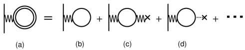
Figure 1: Graphical representation of the baryon density in the self-consistent relativistic Hartree approximation. The double and single lines denote the Hartree propagator and the free propagator of nucleon, respectively. The wavy and dotted lines with cross represnt the vector and scalar potentials given by the previous step of Hartree iteration respectively. The divergence contained in (a) is caused by the contribution from (c).

where $G^{0}$ denotes the Green function for the free Dirac equation. This expansion allows us to write the vacuum polarization as a sum of infinite terms as shown in Fig. 1.

We note that only the second term in the expansion, whose Feynman diagram is depicted in Fig. 1(c), contains an essential divergence of the $\omega$ meson self-energy type. This situation is the same as the vacuum polarization for electron-positron field in QED except for propagating particle is massive and the diagrams including not only vector mesons but also scalar mesons contribute to the correction for baryon density. According to Wichmann and KrollWI56 , the one-loop vacuum correction may be obtained by the sum of the finite part of Fig. 1(c) and Fig. 1(a) subtracted by Fig. 1(c). Thus, the renormalized baryon density from vacuum, $\rho^{VP}_{\omega\hskip 1.42262pt{\rm ren}}(\mathchoice{\mbox{\boldmath$\displaystyle r$}}{\mbox{\boldmath$\textstyle r$}}{\mbox{\boldmath$\scriptstyle r$}}{\mbox{\boldmath$\scriptstyle r$}})$, is written as

$$\rho^{VP}_{\omega\hskip 2.84526pt{\rm ren}}(\mathchoice{\mbox{\boldmath$\displaystyle r$}}{\mbox{\boldmath$\textstyle r$}}{\mbox{\boldmath$\scriptstyle r$}}{\mbox{\boldmath$\scriptstyle r$}})=\rho^{(1)}_{\omega\hskip 2.84526pt{\rm ren}}(\mathchoice{\mbox{\boldmath$\displaystyle r$}}{\mbox{\boldmath$\textstyle r$}}{\mbox{\boldmath$\scriptstyle r$}}{\mbox{\boldmath$\scriptstyle r$}})+\rho^{(R)}_{\omega}(\mathchoice{\mbox{\boldmath$\displaystyle r$}}{\mbox{\boldmath$\textstyle r$}}{\mbox{\boldmath$\scriptstyle r$}}{\mbox{\boldmath$\scriptstyle r$}}),$$ (14)

where $\rho^{(1)}_{\omega\hskip 2.84526pt{\rm ren}}(\mathchoice{\mbox{\boldmath$\displaystyle r$}}{\mbox{\boldmath$\textstyle r$}}{\mbox{\boldmath$\scriptstyle r$}}{\mbox{\boldmath$\scriptstyle r$}})$, which corresponds to the Uehling termUE35 in QED, denotes the finite contribution from Fig. 1(c) and can be calculated from the renormalized result in the momentum representation. Choosing the renormalization point at $q^{2}=0$, only a wave function conterterm $\zeta_{\omega}$ is needed to obtain the finite result:

$$\rho^{(1)}_{\omega\hskip 2.84526pt{\rm ren}}(\mathchoice{\mbox{\boldmath$\displaystyle r$}}{\mbox{\boldmath$\textstyle r$}}{\mbox{\boldmath$\scriptstyle r$}}{\mbox{\boldmath$\scriptstyle r$}})=\int\frac{d\mathchoice{\mbox{\boldmath$\displaystyle p$}}{\mbox{\boldmath$\textstyle p$}}{\mbox{\boldmath$\scriptstyle p$}}{\mbox{\boldmath$\scriptstyle p$}}}{(2\pi)^{3}}e^{i\mathchoice{\mbox{\boldmath$\displaystyle p$}}{\mbox{\boldmath$\textstyle p$}}{\mbox{\boldmath$\scriptstyle p$}}{\mbox{\boldmath$\scriptstyle p$}}\cdot\mathchoice{\mbox{\boldmath$\displaystyle r$}}{\mbox{\boldmath$\textstyle r$}}{\mbox{\boldmath$\scriptstyle r$}}{\mbox{\boldmath$\scriptstyle r$}}}\omega_{0}(\mathchoice{\mbox{\boldmath$\displaystyle p$}}{\mbox{\boldmath$\textstyle p$}}{\mbox{\boldmath$\scriptstyle p$}}{\mbox{\boldmath$\scriptstyle p$}})\frac{g_{\omega}}{\pi^{2}}|\mathchoice{\mbox{\boldmath$\displaystyle p$}}{\mbox{\boldmath$\textstyle p$}}{\mbox{\boldmath$\scriptstyle p$}}{\mbox{\boldmath$\scriptstyle p$}}|^{2}\int_{0}^{1}dxx(1-x)\ln\left(1+\frac{|\mathchoice{\mbox{\boldmath$\displaystyle p$}}{\mbox{\boldmath$\textstyle p$}}{\mbox{\boldmath$\scriptstyle p$}}{\mbox{\boldmath$\scriptstyle p$}}|^{2}x(1-x)}{m_{N}^{2}}\right),$$ (15)

where $\omega_{0}(\mathchoice{\mbox{\boldmath$\displaystyle p$}}{\mbox{\boldmath$\textstyle p$}}{\mbox{\boldmath$\scriptstyle p$}}{\mbox{\boldmath$\scriptstyle p$}})$ is the Fourier transform of $\omega$ meson field $\omega_{0}(\mathchoice{\mbox{\boldmath$\displaystyle r$}}{\mbox{\boldmath$\textstyle r$}}{\mbox{\boldmath$\scriptstyle r$}}{\mbox{\boldmath$\scriptstyle r$}})$. We estimate the contribution from the lowest order of $g_{\omega}^{2}$ by this explicit expression numerically. The second term of Eq. (14), which corresponds to the Wichmann-Kroll termWI56 in QED is the residual finite density expressed by

$$\rho^{(R)}_{\omega}(\mathchoice{\mbox{\boldmath$\displaystyle r$}}{\mbox{\boldmath$\textstyle r$}}{\mbox{\boldmath$\scriptstyle r$}}{\mbox{\boldmath$\scriptstyle r$}}) = \rho^{VP}_{\omega}(\mathchoice{\mbox{\boldmath$\displaystyle r$}}{\mbox{\boldmath$\textstyle r$}}{\mbox{\boldmath$\scriptstyle r$}}{\mbox{\boldmath$\scriptstyle r$}})-\rho^{(1)}_{\omega}(\mathchoice{\mbox{\boldmath$\displaystyle r$}}{\mbox{\boldmath$\textstyle r$}}{\mbox{\boldmath$\scriptstyle r$}}{\mbox{\boldmath$\scriptstyle r$}})$$ (16)

$$= \int_{-i\infty}^{+i\infty}\frac{dz}{2\pi i}{\rm Tr}[\gamma^{0}G^{H}_{V}(\mathchoice{\mbox{\boldmath$\displaystyle r$}}{\mbox{\boldmath$\textstyle r$}}{\mbox{\boldmath$\scriptstyle r$}}{\mbox{\boldmath$\scriptstyle r$}},\mathchoice{\mbox{\boldmath$\displaystyle r$}}{\mbox{\boldmath$\textstyle r$}}{\mbox{\boldmath$\scriptstyle r$}}{\mbox{\boldmath$\scriptstyle r$}};z)]-\int_{-i\infty}^{+i\infty}\frac{dz}{2\pi i}{\rm Tr}[\int d\mathchoice{\mbox{\boldmath$\displaystyle x$}}{\mbox{\boldmath$\textstyle x$}}{\mbox{\boldmath$\scriptstyle x$}}{\mbox{\boldmath$\scriptstyle x$}}\gamma^{0}G^{0}(\mathchoice{\mbox{\boldmath$\displaystyle r$}}{\mbox{\boldmath$\textstyle r$}}{\mbox{\boldmath$\scriptstyle r$}}{\mbox{\boldmath$\scriptstyle r$}},\mathchoice{\mbox{\boldmath$\displaystyle x$}}{\mbox{\boldmath$\textstyle x$}}{\mbox{\boldmath$\scriptstyle x$}}{\mbox{\boldmath$\scriptstyle x$}};z)g_{\omega}\gamma^{0}\omega(\mathchoice{\mbox{\boldmath$\displaystyle x$}}{\mbox{\boldmath$\textstyle x$}}{\mbox{\boldmath$\scriptstyle x$}}{\mbox{\boldmath$\scriptstyle x$}})G^{0}(\mathchoice{\mbox{\boldmath$\displaystyle x$}}{\mbox{\boldmath$\textstyle x$}}{\mbox{\boldmath$\scriptstyle x$}}{\mbox{\boldmath$\scriptstyle x$}},\mathchoice{\mbox{\boldmath$\displaystyle r$}}{\mbox{\boldmath$\textstyle r$}}{\mbox{\boldmath$\scriptstyle r$}}{\mbox{\boldmath$\scriptstyle r$}};z)].$$

In the present work, we evaluate the vacuum correction for baryon density by using this expression directly. After the partial-wave expansion by the Dirac angular-momentum quantum number $\kappa$, each $|\kappa|$ contribution of Eq. (16) is still finite. The partial-wave Green function of RHA calculated numerically on the imaginary axis is used in the first term, while the analytical form of the partial-wave Green function of the free Dirac equation is used in the second term.

There are several advantages to the method solving the Green function on imaginary axis. For example, we can carry out the $z$ integration without taking care of the poles. In addition, we can employ Gaussian quadrature for the radial integral in the second term of right-hand side of Eq. (16) as well as $z$ integration because the Green function on imaginary axis behaves like the modified Bessel function which is not an oscillating function. As a result, the vacuum correction can be obtained very fast with high precision and it is possible to perform the RHA calculation with practical computational time.

It should be noted that $\rho^{(R)}_{\omega}(\mathchoice{\mbox{\boldmath$\displaystyle r$}}{\mbox{\boldmath$\textstyle r$}}{\mbox{\boldmath$\scriptstyle r$}}{\mbox{\boldmath$\scriptstyle r$}})$ contain superficially divergent contribution with the three $\omega$ mesons attached to the baryon loop according to naive power counting, which actually vanishes as a result of current conservation. In QED, how to calculate this term has been discussed by many authors WI56 ; GY72 ; RI75 and it is well known that this contribution vanishes if the summation over $\kappa$ is restricted to a finite number of terms. Then, the $\kappa$ tail contribution is given by the extrapolation. This conclusion is valid for the present case since the neutral $\omega$ meson couples to the conserved baryon current. Hence Eq. (14) together with (15) and (16) can be used to calculate the vacuum correction for the baryon density numerically.

II.3 Vacuum Correction for Scalar Density

Next, we consider the vacuum correction for scalar density. The regularization procedure of scalar density is performed under the same concept as in the baryon density. One can easily see that the perturbative expansion of the Hartree vacuum correction for scalar density corresponding to Eq. (II.2) gives the Feynman diagrams depicted in Fig. 2, where four diagrams from Fig. 2(b) to Fig. 2(e) contain divergent contributions.

The scalar density is renormalized by the counterterms $\alpha_{1}\sigma(\mathchoice{\mbox{\boldmath$\displaystyle r$}}{\mbox{\boldmath$\textstyle r$}}{\mbox{\boldmath$\scriptstyle r$}}{\mbox{\boldmath$\scriptstyle r$}})+1/2\alpha_{2}\sigma^{2}(\mathchoice{\mbox{\boldmath$\displaystyle r$}}{\mbox{\boldmath$\textstyle r$}}{\mbox{\boldmath$\scriptstyle r$}}{\mbox{\boldmath$\scriptstyle r$}})+1/3\alpha_{3}\sigma^{3}(\mathchoice{\mbox{\boldmath$\displaystyle r$}}{\mbox{\boldmath$\textstyle r$}}{\mbox{\boldmath$\scriptstyle r$}}{\mbox{\boldmath$\scriptstyle r$}})+1/4\alpha_{4}\sigma^{4}(\mathchoice{\mbox{\boldmath$\displaystyle r$}}{\mbox{\boldmath$\textstyle r$}}{\mbox{\boldmath$\scriptstyle r$}}{\mbox{\boldmath$\scriptstyle r$}})+1/2\zeta_{\sigma}\partial_{\mu}\sigma(\mathchoice{\mbox{\boldmath$\displaystyle r$}}{\mbox{\boldmath$\textstyle r$}}{\mbox{\boldmath$\scriptstyle r$}}{\mbox{\boldmath$\scriptstyle r$}})\partial^{\mu}\sigma(\mathchoice{\mbox{\boldmath$\displaystyle r$}}{\mbox{\boldmath$\textstyle r$}}{\mbox{\boldmath$\scriptstyle r$}}{\mbox{\boldmath$\scriptstyle r$}})$ in $\delta{\cal L}$. The finite part of Fig. 2(c) is calculated from the renormalized result in the vacuum. The mass ($\alpha_{2}$) and wave function ($\zeta_{\sigma}$) counterterms are required to make the contribution finite. The result is given by

$$\rho^{(1)}_{\sigma\hskip 2.84526pt{\rm ren}}(\mathchoice{\mbox{\boldmath$\displaystyle r$}}{\mbox{\boldmath$\textstyle r$}}{\mbox{\boldmath$\scriptstyle r$}}{\mbox{\boldmath$\scriptstyle r$}})=\int\frac{d\mathchoice{\mbox{\boldmath$\displaystyle p$}}{\mbox{\boldmath$\textstyle p$}}{\mbox{\boldmath$\scriptstyle p$}}{\mbox{\boldmath$\scriptstyle p$}}}{(2\pi)^{3}}e^{i\mathchoice{\mbox{\boldmath$\displaystyle p$}}{\mbox{\boldmath$\textstyle p$}}{\mbox{\boldmath$\scriptstyle p$}}{\mbox{\boldmath$\scriptstyle p$}}\cdot\mathchoice{\mbox{\boldmath$\displaystyle r$}}{\mbox{\boldmath$\textstyle r$}}{\mbox{\boldmath$\scriptstyle r$}}{\mbox{\boldmath$\scriptstyle r$}}}\sigma(\mathchoice{\mbox{\boldmath$\displaystyle p$}}{\mbox{\boldmath$\textstyle p$}}{\mbox{\boldmath$\scriptstyle p$}}{\mbox{\boldmath$\scriptstyle p$}})\frac{3g^{2}_{\sigma}}{2\pi^{2}}\left[\frac{1}{6}|\mathchoice{\mbox{\boldmath$\displaystyle p$}}{\mbox{\boldmath$\textstyle p$}}{\mbox{\boldmath$\scriptstyle p$}}{\mbox{\boldmath$\scriptstyle p$}}|^{2}-\int_{0}^{1}dx(m_{N}^{2}+|\mathchoice{\mbox{\boldmath$\displaystyle p$}}{\mbox{\boldmath$\textstyle p$}}{\mbox{\boldmath$\scriptstyle p$}}{\mbox{\boldmath$\scriptstyle p$}}|^{2}x(1-x))\ln\left(1+\frac{|\mathchoice{\mbox{\boldmath$\displaystyle p$}}{\mbox{\boldmath$\textstyle p$}}{\mbox{\boldmath$\scriptstyle p$}}{\mbox{\boldmath$\scriptstyle p$}}|^{2}x(1-x)}{m_{N}^{2}}\right)\right],$$ (17)

where $\sigma(\mathchoice{\mbox{\boldmath$\displaystyle p$}}{\mbox{\boldmath$\textstyle p$}}{\mbox{\boldmath$\scriptstyle p$}}{\mbox{\boldmath$\scriptstyle p$}})$ is the Fourier transform of $\sigma(\mathchoice{\mbox{\boldmath$\displaystyle r$}}{\mbox{\boldmath$\textstyle r$}}{\mbox{\boldmath$\scriptstyle r$}}{\mbox{\boldmath$\scriptstyle r$}})$ and we have chosen $q^{2}=0$ for the renormalization point. The physical vacuum contribution for scalar density is given by the sum of $\rho^{(1)}_{\sigma\hskip 2.84526pt{\rm ren}}(\mathchoice{\mbox{\boldmath$\displaystyle r$}}{\mbox{\boldmath$\textstyle r$}}{\mbox{\boldmath$\scriptstyle r$}}{\mbox{\boldmath$\scriptstyle r$}})$ and the residual finite density denoted by $\rho^{(R)}_{\sigma}(\mathchoice{\mbox{\boldmath$\displaystyle r$}}{\mbox{\boldmath$\textstyle r$}}{\mbox{\boldmath$\scriptstyle r$}}{\mbox{\boldmath$\scriptstyle r$}})$:

$$\rho^{VP}_{\sigma\hskip 2.84526pt{\rm ren}}(\mathchoice{\mbox{\boldmath$\displaystyle r$}}{\mbox{\boldmath$\textstyle r$}}{\mbox{\boldmath$\scriptstyle r$}}{\mbox{\boldmath$\scriptstyle r$}})=\rho^{(1)}_{\sigma\hskip 2.84526pt{\rm ren}}(\mathchoice{\mbox{\boldmath$\displaystyle r$}}{\mbox{\boldmath$\textstyle r$}}{\mbox{\boldmath$\scriptstyle r$}}{\mbox{\boldmath$\scriptstyle r$}})+\rho^{(R)}_{\sigma}(\mathchoice{\mbox{\boldmath$\displaystyle r$}}{\mbox{\boldmath$\textstyle r$}}{\mbox{\boldmath$\scriptstyle r$}}{\mbox{\boldmath$\scriptstyle r$}}).$$ (18)

where the residual finite density $\rho^{(R)}_{\sigma}(\mathchoice{\mbox{\boldmath$\displaystyle r$}}{\mbox{\boldmath$\textstyle r$}}{\mbox{\boldmath$\scriptstyle r$}}{\mbox{\boldmath$\scriptstyle r$}})$ includes the finite contributions arising from Figs. 2(b), 2(d), and 2(e). The finite residual vacuum density $\rho^{(R)}_{\sigma}(\mathchoice{\mbox{\boldmath$\displaystyle r$}}{\mbox{\boldmath$\textstyle r$}}{\mbox{\boldmath$\scriptstyle r$}}{\mbox{\boldmath$\scriptstyle r$}})$ is evaluated by subtracting the contribution of Fig. 2(c) and the counterterms from the unrenormalized divergent scalar density:

$$\rho^{(R)}_{\sigma}(\mathchoice{\mbox{\boldmath$\displaystyle r$}}{\mbox{\boldmath$\textstyle r$}}{\mbox{\boldmath$\scriptstyle r$}}{\mbox{\boldmath$\scriptstyle r$}}) = \int_{-i\infty}^{+i\infty}\frac{dz}{2\pi i}{\rm Tr}[G^{H}_{V}(\mathchoice{\mbox{\boldmath$\displaystyle r$}}{\mbox{\boldmath$\textstyle r$}}{\mbox{\boldmath$\scriptstyle r$}}{\mbox{\boldmath$\scriptstyle r$}},\mathchoice{\mbox{\boldmath$\displaystyle r$}}{\mbox{\boldmath$\textstyle r$}}{\mbox{\boldmath$\scriptstyle r$}}{\mbox{\boldmath$\scriptstyle r$}};z)]$$ (19)

$$-\int_{-i\infty}^{+i\infty}\frac{dz}{2\pi i}{\rm Tr}[\int d\mathchoice{\mbox{\boldmath$\displaystyle x$}}{\mbox{\boldmath$\textstyle x$}}{\mbox{\boldmath$\scriptstyle x$}}{\mbox{\boldmath$\scriptstyle x$}}G^{0}(\mathchoice{\mbox{\boldmath$\displaystyle r$}}{\mbox{\boldmath$\textstyle r$}}{\mbox{\boldmath$\scriptstyle r$}}{\mbox{\boldmath$\scriptstyle r$}},\mathchoice{\mbox{\boldmath$\displaystyle x$}}{\mbox{\boldmath$\textstyle x$}}{\mbox{\boldmath$\scriptstyle x$}}{\mbox{\boldmath$\scriptstyle x$}};z)g_{\sigma}\sigma(\mathchoice{\mbox{\boldmath$\displaystyle x$}}{\mbox{\boldmath$\textstyle x$}}{\mbox{\boldmath$\scriptstyle x$}}{\mbox{\boldmath$\scriptstyle x$}})G^{0}(\mathchoice{\mbox{\boldmath$\displaystyle x$}}{\mbox{\boldmath$\textstyle x$}}{\mbox{\boldmath$\scriptstyle x$}}{\mbox{\boldmath$\scriptstyle x$}},\mathchoice{\mbox{\boldmath$\displaystyle r$}}{\mbox{\boldmath$\textstyle r$}}{\mbox{\boldmath$\scriptstyle r$}}{\mbox{\boldmath$\scriptstyle r$}};z)]$$

$$-(\alpha_{1}+\alpha_{3}\sigma^{2}(\mathchoice{\mbox{\boldmath$\displaystyle r$}}{\mbox{\boldmath$\textstyle r$}}{\mbox{\boldmath$\scriptstyle r$}}{\mbox{\boldmath$\scriptstyle r$}})+\alpha_{4}\sigma^{3}(\mathchoice{\mbox{\boldmath$\displaystyle r$}}{\mbox{\boldmath$\textstyle r$}}{\mbox{\boldmath$\scriptstyle r$}}{\mbox{\boldmath$\scriptstyle r$}}))/g_{\sigma},$$

where the coefficients $\alpha_{1},\alpha_{3}$, and $\alpha_{4}$ of the counterterms are given by

$$\alpha_{1} = g_{\sigma}\int_{-i\infty}^{+i\infty}\frac{dz}{2\pi i}{\rm Tr}[G^{0}(\mathchoice{\mbox{\boldmath$\displaystyle r$}}{\mbox{\boldmath$\textstyle r$}}{\mbox{\boldmath$\scriptstyle r$}}{\mbox{\boldmath$\scriptstyle r$}},\mathchoice{\mbox{\boldmath$\displaystyle r$}}{\mbox{\boldmath$\textstyle r$}}{\mbox{\boldmath$\scriptstyle r$}}{\mbox{\boldmath$\scriptstyle r$}};z)]$$ (20)

$$\alpha_{3} = g_{\sigma}^{3}\int_{-i\infty}^{+i\infty}\frac{dz}{2\pi i}{\rm Tr}[\int d\mathchoice{\mbox{\boldmath$\displaystyle x_{1}$}}{\mbox{\boldmath$\textstyle x_{1}$}}{\mbox{\boldmath$\scriptstyle x_{1}$}}{\mbox{\boldmath$\scriptstyle x_{1}$}}d\mathchoice{\mbox{\boldmath$\displaystyle x_{2}$}}{\mbox{\boldmath$\textstyle x_{2}$}}{\mbox{\boldmath$\scriptstyle x_{2}$}}{\mbox{\boldmath$\scriptstyle x_{2}$}}G^{0}(\mathchoice{\mbox{\boldmath$\displaystyle r$}}{\mbox{\boldmath$\textstyle r$}}{\mbox{\boldmath$\scriptstyle r$}}{\mbox{\boldmath$\scriptstyle r$}},\mathchoice{\mbox{\boldmath$\displaystyle x_{1}$}}{\mbox{\boldmath$\textstyle x_{1}$}}{\mbox{\boldmath$\scriptstyle x_{1}$}}{\mbox{\boldmath$\scriptstyle x_{1}$}};z)G^{0}(\mathchoice{\mbox{\boldmath$\displaystyle x_{1}$}}{\mbox{\boldmath$\textstyle x_{1}$}}{\mbox{\boldmath$\scriptstyle x_{1}$}}{\mbox{\boldmath$\scriptstyle x_{1}$}},\mathchoice{\mbox{\boldmath$\displaystyle x_{2}$}}{\mbox{\boldmath$\textstyle x_{2}$}}{\mbox{\boldmath$\scriptstyle x_{2}$}}{\mbox{\boldmath$\scriptstyle x_{2}$}};z)G^{0}(\mathchoice{\mbox{\boldmath$\displaystyle x_{2}$}}{\mbox{\boldmath$\textstyle x_{2}$}}{\mbox{\boldmath$\scriptstyle x_{2}$}}{\mbox{\boldmath$\scriptstyle x_{2}$}},\mathchoice{\mbox{\boldmath$\displaystyle r$}}{\mbox{\boldmath$\textstyle r$}}{\mbox{\boldmath$\scriptstyle r$}}{\mbox{\boldmath$\scriptstyle r$}};z)]$$ (21)

$$\alpha_{4} = g_{\sigma}^{4}\int_{-i\infty}^{+i\infty}\frac{dz}{2\pi i}{\rm Tr}[\int d\mathchoice{\mbox{\boldmath$\displaystyle x_{1}$}}{\mbox{\boldmath$\textstyle x_{1}$}}{\mbox{\boldmath$\scriptstyle x_{1}$}}{\mbox{\boldmath$\scriptstyle x_{1}$}}d\mathchoice{\mbox{\boldmath$\displaystyle x_{2}$}}{\mbox{\boldmath$\textstyle x_{2}$}}{\mbox{\boldmath$\scriptstyle x_{2}$}}{\mbox{\boldmath$\scriptstyle x_{2}$}}d\mathchoice{\mbox{\boldmath$\displaystyle x_{3}$}}{\mbox{\boldmath$\textstyle x_{3}$}}{\mbox{\boldmath$\scriptstyle x_{3}$}}{\mbox{\boldmath$\scriptstyle x_{3}$}}G^{0}(\mathchoice{\mbox{\boldmath$\displaystyle r$}}{\mbox{\boldmath$\textstyle r$}}{\mbox{\boldmath$\scriptstyle r$}}{\mbox{\boldmath$\scriptstyle r$}},\mathchoice{\mbox{\boldmath$\displaystyle x_{1}$}}{\mbox{\boldmath$\textstyle x_{1}$}}{\mbox{\boldmath$\scriptstyle x_{1}$}}{\mbox{\boldmath$\scriptstyle x_{1}$}};z)G^{0}(\mathchoice{\mbox{\boldmath$\displaystyle x_{1}$}}{\mbox{\boldmath$\textstyle x_{1}$}}{\mbox{\boldmath$\scriptstyle x_{1}$}}{\mbox{\boldmath$\scriptstyle x_{1}$}},\mathchoice{\mbox{\boldmath$\displaystyle x_{2}$}}{\mbox{\boldmath$\textstyle x_{2}$}}{\mbox{\boldmath$\scriptstyle x_{2}$}}{\mbox{\boldmath$\scriptstyle x_{2}$}};z)G^{0}(\mathchoice{\mbox{\boldmath$\displaystyle x_{2}$}}{\mbox{\boldmath$\textstyle x_{2}$}}{\mbox{\boldmath$\scriptstyle x_{2}$}}{\mbox{\boldmath$\scriptstyle x_{2}$}},\mathchoice{\mbox{\boldmath$\displaystyle x_{3}$}}{\mbox{\boldmath$\textstyle x_{3}$}}{\mbox{\boldmath$\scriptstyle x_{3}$}}{\mbox{\boldmath$\scriptstyle x_{3}$}};z)G^{0}(\mathchoice{\mbox{\boldmath$\displaystyle x_{3}$}}{\mbox{\boldmath$\textstyle x_{3}$}}{\mbox{\boldmath$\scriptstyle x_{3}$}}{\mbox{\boldmath$\scriptstyle x_{3}$}},\mathchoice{\mbox{\boldmath$\displaystyle r$}}{\mbox{\boldmath$\textstyle r$}}{\mbox{\boldmath$\scriptstyle r$}}{\mbox{\boldmath$\scriptstyle r$}};z)].$$ (22)

We note that $\alpha_{1}$, $\alpha_{3}$, and $\alpha_{4}$ are independent of $\textstyle r$ though it remains in the right-hand side of these expressions. Performing the partial-wave expansion of free Green functions, however, each $|\kappa|$ contribution to the coefficients depends on the radial part $r$. With these partial-wave subtraction terms, the scalar density is calculated for each $|\kappa|$. The net effect of scalar density generated from the vacuum polarization are obtained by taking the extrapolation $|\kappa_{max}|\rightarrow\infty$.

III Computational detail for vacuum correction

As has been explained in the previous section, $\rho^{(1)}_{\omega\hskip 2.84526pt{\rm ren}}$ and $\rho^{(1)}_{\sigma\hskip 2.84526pt{\rm ren}}$ contributions are calculated from the explicit forms (15) and (17). They contribute by a small amount as discussed below. Therefore, here we explain mainly the estimation of the residual contributions defined by Eqs. (16) and (19). We write the radial part of the residual baryon and scalar densities as

$$\rho^{R}_{\omega\hskip 2.84526pt{\rm ren}}({r})=\sum_{|\kappa|=1}^{|\kappa_{max}|}\rho^{R}_{\omega\hskip 1.42262pt{\rm ren},|\kappa|}({r})$$ (23)

and

$$\rho^{R}_{\sigma\hskip 2.84526pt{\rm ren}}({r})=\sum_{|\kappa|=1}^{|\kappa_{max}|}\rho^{R}_{\sigma\hskip 1.42262pt{\rm ren},|\kappa|}({r}),$$ (24)

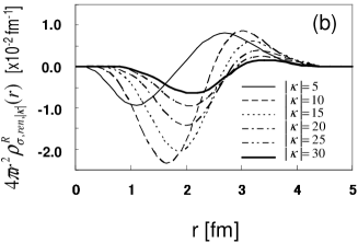
Figure 3: The contributions from $|\kappa|=$5, 10, 15, 20, 25, and 30 to (a) the baryon density $\rho^{R}_{\omega\hskip 1.42262pt{\rm ren},|\kappa|}({r})$ and (b) the scalar density $\rho^{R}_{\sigma\hskip 1.42262pt{\rm ren},|\kappa|}({r})$.

respectively. Here, $\rho^{R}_{\omega\hskip 1.42262pt{\rm ren},|\kappa|}$ ($\rho^{R}_{\sigma\hskip 1.42262pt{\rm ren},|\kappa|}$) represents the contribution from $|\kappa|=\pm\kappa$ to net residual baryon (scalar) density. We compute $\rho^{R}_{\omega\hskip 1.42262pt{\rm ren},|\kappa|}$ and $\rho^{R}_{\sigma\hskip 1.42262pt{\rm ren},|\kappa|}$ using the angular momentum decomposed expression of Eqs. (16) and (19). The detail of our calculation is the following. For the respective contributions of $|\kappa|$ in Eqs. (16) and (19), we carry out the integral over $iz$ using Gaussian quadrature. The radial Green functions with the imaginary energy are given in terms of the two solutions of the Dirac equation; the solution regular at $r=0$ and the solution regular at $r=\infty$. Several values of the upper and lower limits of the integral over $z$ are selected depending on the radius parameter $r$ around $20i\sim 50i$ GeV. The vacuum densities $\rho^{R}_{\omega\hskip 1.42262pt{\rm ren},|\kappa|}({r})$ and $\rho^{R}_{\sigma\hskip 1.42262pt{\rm ren},|\kappa|}({r})$ for $z_{max}\rightarrow\infty$ are extrapolated from the resulting integrated values. Then, the sum over $|\kappa|$ is performed until the cutoff $|\kappa_{max}|$. The sum over $|\kappa|$ does not converge so rapidly. In the present work, $|\kappa_{max}|$ in baryon density is 33 for both of ¹⁶O and ⁴⁰Ca, while $|\kappa_{max}|$ in scalar density is 36 for ¹⁶O and 48 for ⁴⁰Ca. Finally, we have extrapolated $|\kappa|$ contribution to larger values to obtain the convergent vacuum densities. As an example, the contributions from $|\kappa|=$5, 10, 15, 20, 25, and 30 for in ¹⁶O are shown in Fig. 3.

An accuracy test for the computed vacuum correction of the baryon density $\rho^{R}_{\omega\hskip 1.42262pt{\rm ren}}({r})$ is provided by the requirement that for the total induced vacuum correction should vanish due to the conservation of baryon density,

$$\Delta B=4\pi\int_{0}^{\infty}drr^{2}\rho^{R}_{\omega\hskip 1.42262pt{\rm ren}}({r})=0.$$ (25)

In the present calculation with various QHD parameters, we found $\Delta B\sim 10^{-3}$ as a typical values both for ¹⁶O and ⁴⁰Ca. For the scalar density, on the other hand, we have no requirement of conservation laws. However, it would be reasonable to expect the numerical error in scalar density is of the same order of magnitude as the one in the baryon density.

In Sec. II.B, we mentioned that the divergence of unrenormalized baryon density in the present model has the same structure as unrenormalized vacuum charge density of electron-positron field in the QED correction. However, the dependence on the partial-wave contribution is largely different from the QED case: a large $|\kappa_{max}|$ is required to achieve the convergence as seen in Fig. 3, while for the renormalized charge density in QED only the term with $|\kappa_{max}|=1$ is a good approximationGY72 . In addition, it should be pointed out that Eqs. (15) and (17) are negligible in the present calculation, namely, $\rho^{(1)}_{\omega\hskip 2.84526pt{\rm ren}}$ and $\rho^{(1)}_{\sigma\hskip 2.84526pt{\rm ren}}$ are an order of magnitude smaller than the residual densities in contrast with the QED calculation, in which the corresponding contribution known as the Uehling effect has a dominant contributionRI75 . These differences from QED seem to be caused by the $\omega-\sigma$ couplings as well as the large coupling constant of the nuclear force. In particular, the baryon density, the source of the $\omega$ meson, is strongly influenced by the $\sigma$ meson. This is shown in Fig. 4 where the baryon densities $\rho^{(1)}_{\omega\hskip 2.84526pt{\rm ren}}(r)$ with and without $\sigma$ meson are compared. We can see there that the vacuum correction for baryon density is negligibly small if the $\omega$ meson only is taken into account. We found that the baryon density induced by the vacuum polarization comes from the diagrams with $\sigma$ meson self-energy insertions mainly.

IV Results and Discussion

Here we show the results of the relativistic Hartree calculation with a rigorous treatment of renormalized densities in ¹⁶O and ⁴⁰Ca based on the Lagrangian density of Eq. (1). The numerical procedure of the present RHA calculation is similar to that used in the conventional RMF calculation: first, the Dirac equation (3) for only the valence nucleons is solved under the external $\omega$ and $\sigma$ fields. Second, using the same potential, we calculate vacuum densities by means of the Green function described in the previous section. Third, the equations of motion of mesons, (6) and (7), are solved with the source terms due to the valence nucleons and vacuum contributions. Substituting these results in the Dirac equation, we complete one iteration step. Using the same method as indicated in the previous section, the energy shift due to the vacuum polarization is estimated by

$$E_{VP} = \int d\mathchoice{\mbox{\boldmath$\displaystyle r$}}{\mbox{\boldmath$\textstyle r$}}{\mbox{\boldmath$\scriptstyle r$}}{\mbox{\boldmath$\scriptstyle r$}}\left[\int_{-i\infty}^{+i\infty}\frac{dz}{2\pi i}{\rm Tr}[\gamma^{0}\left(G^{H}_{V}(\mathchoice{\mbox{\boldmath$\displaystyle r$}}{\mbox{\boldmath$\textstyle r$}}{\mbox{\boldmath$\scriptstyle r$}}{\mbox{\boldmath$\scriptstyle r$}},\mathchoice{\mbox{\boldmath$\displaystyle r$}}{\mbox{\boldmath$\textstyle r$}}{\mbox{\boldmath$\scriptstyle r$}}{\mbox{\boldmath$\scriptstyle r$}};z)-G^{0}(\mathchoice{\mbox{\boldmath$\displaystyle r$}}{\mbox{\boldmath$\textstyle r$}}{\mbox{\boldmath$\scriptstyle r$}}{\mbox{\boldmath$\scriptstyle r$}},\mathchoice{\mbox{\boldmath$\displaystyle r$}}{\mbox{\boldmath$\textstyle r$}}{\mbox{\boldmath$\scriptstyle r$}}{\mbox{\boldmath$\scriptstyle r$}};z)\right)]z+(CT)\right],$$ (27)

$$CT=-1/4\zeta_{\omega}(\mathchoice{\mbox{\boldmath$\displaystyle\nabla$}}{\mbox{\boldmath$\textstyle\nabla$}}{\mbox{\boldmath$\scriptstyle\nabla$}}{\mbox{\boldmath$\scriptstyle\nabla$}}\omega_{0})^{2}+1/2\zeta_{\sigma}(\mathchoice{\mbox{\boldmath$\displaystyle\nabla$}}{\mbox{\boldmath$\textstyle\nabla$}}{\mbox{\boldmath$\scriptstyle\nabla$}}{\mbox{\boldmath$\scriptstyle\nabla$}}\sigma)^{2}+\alpha_{1}\sigma+1/2\alpha_{2}\sigma^{2}+1/3\alpha_{3}\sigma^{3}+1/4\alpha_{4}\sigma^{4},$$

is calculated at each step of iteration. The iteration is continued until the total binding energy of the nucleus $E_{\rm{total}}=E_{\rm{meson}}+E_{\rm{valence}}+E_{VP}$ converges showing self consistency.

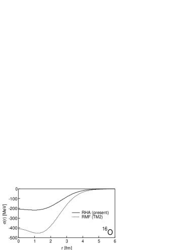
Figure 5: The scalar potentials for ¹⁶O in the left panel and for ⁴⁰Ca in the right panel. The scalar potential with the vacuum polarization is shown by solid curve, while the one without it by dashed curve.

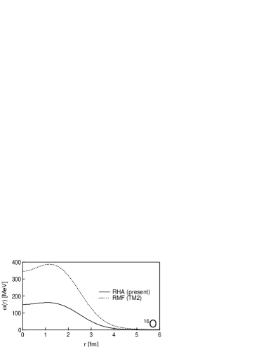
Figure 6: The vector potentials for ¹⁶O in the left panel and for ⁴⁰Ca in the right panel. The scalar potential with the vacuum polarization is shown by solid curve, while the one without it by dashed curve.

The QHD parameter set is chosen so as to reproduce reasonably well the experimental values of the total binding energies, the rms radii, and the single-particle energies for both of ¹⁶O and ⁴⁰Ca. In the second column of Table I, we give the results with the coupling constants and masses $g_{\sigma}=7.38$, $g_{2}=7.90$, $g_{3}=3.20$, and $m_{\sigma}=458.0$ MeV for $\sigma$ meson, and $g_{\omega}=9.18$ and $m_{\omega}=783.0$ MeV for $\omega$ meson. The results of the RMF calculation with the parameter set TM2SU94 and experimental data taken from Ref. DATA are also shown in the third and last columns, respectively. We see that our total binding energies including the vacuum correction and rms radii are similar to those of RMF and agree with the experimental data well. However, it should be noted that the present result is produced by using smaller coupling constants than those of RMF. Hence, the scalar and vector potentials in the present RHA differ considerably from those of RMF. The results of the present RHA in ¹⁶O and ⁴⁰Ca are compared with the results of RMF in Figs. 5 and 6 for scalar and vector potentials, respectively. One can see that the fields in the RHA are considerably small compared with those in the RMF.

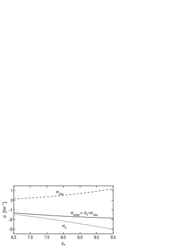
Figure 7: The scalar potential in nuclear matter. $\sigma$ meson mass $m_{\sigma}=458.0$ and Fermi momentum $k_{F}=1.42$ are employed. $\sigma_{0}$ denotes the ordinary $\sigma$ meson field generated from the valence nucleons while $\sigma_{Vac}$ denotes the contribution from the vacuum. Due to the cancellation between them, the net $\sigma$ meson field does not increase smoothly with the coupling constant, $g_{\sigma}$.

The vacuum contribution plays a crucial role for the generation of the weak meson fields. In order to see this, we plot $\sigma$-meson field in nuclear matter as a function of the coupling constant $g_{\sigma}$ while keeping the other parameters fixed in Fig. 7. The figure shows that the vacuum correction contributes destructively to the valence contribution and it is impossible to obtain a strong meson field unless a very large coupling constant is used. Of course, we could choose a parameter set with large coupling constants. However, such a parameter set would have produced an unstable solution in the RHA calculation, because if the deeply-bound antinucleon states are produced by the strong $\omega$ and $\sigma$ fields with large coupling constants, then the vacuum effect, which works in the opposite direction, also becomes large to suppress the strong fields. Such a RHA solution is not realistic because it is unstable even for the trivial fluctuation of the density. Thus, we have to choose a parameter set which produces a weak field in the self consistent iteration.

The RMF reproduces reasonably well the observed tendency of the single-particle spectra due to the small effective mass of the nucleon, $m^{*}_{N}(r)=m_{N}+g_{\sigma}\sigma(r)$. The fact that the scalar field is suppressed in RHA results in the large effective mass. As a result, it raises a problem in fitting the single-particle energies. As seen in Table I, the energy splittings in the single-particle states of the present RHA are very small and they are unlikely to agree with the experimental values. This problem has been already known by RHA calculation using the local-density approximation and the derivative expansion to estimate the vacuum correctionWA88 ; MA99 . It is difficult to resolve this problem by RHA with ordinary QHD models used up to now.

Thus, the QHD models require a mechanism for the spin-orbit splittings other than the small effective mass. One suggestion is made in Refs. MA03 ; SU942 , where a tensor-coupling of $\omega$ meson is introduced in order to provide the spin-orbit splittings. However, the omega meson coupling with the nucleon is known to be dominated by the vector coupling in the nucleon-nucleon potential. Another candidate to solve this problem may be the possibility of the finite pion mean field in the relativistic Hartree framework, which was suggested to provide the spin up and spin down partners to have large energy separationsOG04 . It is interesting to extend the present RHA calculation with these effects taken into account. This is certainly a subject to be worked out in future study.

V Comparison with the previous method for vacuum polarization

The effect of the negative-energy nucleons for finite nuclei was first estimated by the local-density approximationHO84 ; IC88 ; FO89 . It was developed further by applying the derivative-expansion method PE86 ; WA88 ; MA99 ; MA03 . In this section, we compare our results densities induced by the vacuum polarization with those of the local-density approximation and the derivative-expansion method. The local-density approximation uses as input the result of the infinite nuclear matter. In this approximation, the vacuum correction is given by

$$\rho_{\sigma,ren}^{VP(LDA)}(r)=-\frac{1}{\pi^{2}}\left[m^{*3}_{N}\ln(m^{*}_{N}/m_{N})+1/3m_{N}^{3}-3/2m_{N}^{2}m^{*}_{N}+3m_{N}m^{*2}_{N}-11/6m^{*3}_{N}\right],$$ (28)

and decreases the scalar density in nuclear interior. The vacuum does not change the baryon density because of the conservation of the baryon number. In the derivative-expansion method, on the other hand, the presence of the derivative term allows non-vanishing correction for baryon density as well as for scalar density:

$$\rho_{\omega,ren}^{VP(DE)}(r) = -\frac{g_{\omega}}{3\pi^{2}}\mathchoice{\mbox{\boldmath$\displaystyle\nabla$}}{\mbox{\boldmath$\textstyle\nabla$}}{\mbox{\boldmath$\scriptstyle\nabla$}}{\mbox{\boldmath$\scriptstyle\nabla$}}\cdot\ln\left(\frac{m_{N}^{*}(r)}{m_{N}}\right)\mathchoice{\mbox{\boldmath$\displaystyle\nabla$}}{\mbox{\boldmath$\textstyle\nabla$}}{\mbox{\boldmath$\scriptstyle\nabla$}}{\mbox{\boldmath$\scriptstyle\nabla$}}\omega_{0}(r),$$ (29)

$$\rho_{\sigma,ren}^{VP(DE)}(r) = \rho_{\sigma,ren}^{VP(LDA)}(r)-\frac{g_{\sigma}}{2\pi^{2}}\mathchoice{\mbox{\boldmath$\displaystyle\nabla$}}{\mbox{\boldmath$\textstyle\nabla$}}{\mbox{\boldmath$\scriptstyle\nabla$}}{\mbox{\boldmath$\scriptstyle\nabla$}}\cdot\ln\left(\frac{m_{N}^{*}(r)}{m_{N}}\right)\mathchoice{\mbox{\boldmath$\displaystyle\nabla$}}{\mbox{\boldmath$\textstyle\nabla$}}{\mbox{\boldmath$\scriptstyle\nabla$}}{\mbox{\boldmath$\scriptstyle\nabla$}}\sigma(r)$$ (30)

$$-\frac{g_{\sigma}^{2}}{4\pi^{2}m_{N}^{*}(r)}(\mathchoice{\mbox{\boldmath$\displaystyle\nabla$}}{\mbox{\boldmath$\textstyle\nabla$}}{\mbox{\boldmath$\scriptstyle\nabla$}}{\mbox{\boldmath$\scriptstyle\nabla$}}\sigma(r))^{2}+\frac{g_{\omega}^{2}}{6\pi^{2}m_{N}^{*}(r)}(\mathchoice{\mbox{\boldmath$\displaystyle\nabla$}}{\mbox{\boldmath$\textstyle\nabla$}}{\mbox{\boldmath$\scriptstyle\nabla$}}{\mbox{\boldmath$\scriptstyle\nabla$}}\omega(r))^{2},$$

where the leading order of the derivative terms is taken into account. The baryon and scalar densities induced by the vacuum polarization are given in Fig. 8, together with those from the local-density approximation and the derivative expansion. For purpose of comparison, we assume there the same potential in evaluating the vacuum polarization. We can see that the densities obtained by the local-density approximation are corrected significantly not only for baryon density, which vanishes in this approximation, but also for scalar density. The both of scalar and baryon density-profiles obtained by the present calculation are in a surprisingly good agreement with those of the derivative expansion.

However, this cannot be always the caseST97 and it is possible to attribute the excellent agreement between our method and the leading-order derivative expansion to the character of $\sigma-\omega$ model. Consider, for example, the vacuum correction in the baryon density without $\sigma$ meson. In this situation, the vacuum correction using the present method can be significant with large coupling constant of $\omega$ meson. As found in Eq. (29), on the other hand, the vacuum correction from the derivative expansion vanishes exactly for $m_{N}^{*}(r)\rightarrow m_{N}$. Hence, we find that $\sigma$ meson plays important role in the agreement between our method and the leading-order derivative expansion. Thus, the present calculation supports that leading-order derivative expansion is greatly useful for the estimation of the vacuum correction in RHA.

In the present calculation of the full RHA for finite nuclei, the vacuum-polarization corrections (15) and (17) to the meson propagators are implicitly taken into account to all orders through iteration to achieve the self-consistency in the relativistic Hartree approximation. There the unphysical pole in the meson propagator at finite momentum transfer, known as Landau ghost, may affect the present numerical resultsIC88 ; KT91 through integration over the momentum transfer. However, this unphysical effect is not significant in the RHA of finite nuclei, because even if the (15) and (17) terms are totally ignored in the calculation, the final results of scalar and vector densities do not change appreciably. The good agreement with the results of the derivative expansion, where the Landau ghost plays no role, also implies that the unphysical effect is negligible.

VI Summary

We have developed a rigorous method to calculate vacuum-polarization effects in relativistic Hartree approach. The renormalized baryon and scalar densities have been evaluated within a practical computational time replacing the summation of the Hartree basis by the numerical integral of the Dirac Green function over the imaginary energy. We have obtained numerical results that the vacuum corrections for baryon and scalar densities are non-negligible in the RHA calculation. In particular, we have seen that the vector and scalar potentials in the RHA are largely suppressed by the feedback of the vacuum polarization to the mean fields. Such suppressed potentials of the $\omega$ and $\sigma$ fields affect the theoretical calculations for binding energies of antinucleon and the various sum rules.

Our results with the Walecka model have reproduced the experimental binding energies and rms radii of ¹⁶O and ⁴⁰Ca nicely after adjusting the parameters. However, it was impossible to find a QHD parameter set to reproduce spin-orbit splittings in accordance with the observed data and required by nuclear shell model. In the $\sigma-\omega$ model, the main attraction is caused by the large $\sigma$ mean field, which provides small nucleon effective mass in the finite nuclei. However, the negative-energy nucleons do not like to change its mass from the free value. Hence, the negative-energy nucleons try to keep the nucleon mass at the free value. For the net effect, the effective nucleon mass remains to be quite large. Once the effective nucleon mass becomes large, the spin-orbit splittings in the single particle spectra come out to be very small. The QHD type effective theory based on the $\sigma-\omega$ mesons need to include new type of interaction terms and/or to go beyond the RHA approximation to solve this problem.

We have found that our result of RHA calculation is very similar to that in Refs. PE86 ; MA99 where the derivative-expansion method was used to estimate the vacuum polarization. In particular, it has been shown that the agreement of density-profiles of the vacuum correction is quite good. Thus, the validity of this approximation has been confirmed by the present calculation.

This work has been supported by MATSUO FOUNDATION, Suginami, Tokyo. A.H. would like to thank Prof. S. Kita and Prof. Y. Tanaka for giving him the opportunity to do this work and useful discussion. Y.H. acknowledges Dr. K. Tanaka for useful discussion.

TABLE I. The total binding energies, the rms charge radii, and the single-particle energies in ¹⁶O and ⁴⁰Ca.
$\begin{array}[]{lcccc}\hline\cr\hline\cr&\hskip 28.45274pt{\rm Present\hskip 2.84526ptRHA}&\hskip 28.45274pt{\rm TM2}&\hskip 28.45274pt{\rm Experiment}&\\ \hline\cr{}^{16}{\rm O}\\ E_{\rm total}/A(E_{VP}/A)\hskip 2.84526pt{\rm[MeV]}&8.05(1.69)&7.93(-)&7.98(-)\\ r_{ch}\hskip 2.84526pt{\rm[fm]}&2.65&2.67&2.74\\ {\rm Single\hskip 2.84526ptparticle\hskip 2.84526ptstate\hskip 2.84526ptof\hskip 2.84526ptproton}\\ 1s_{1/2}{\rm[MeV]}&31.0&38.2&40\pm 8\\ 1p_{3/2}{\rm[MeV]}&15.6&18.6&18.4\\ 1p_{1/2}{\rm[MeV]}&13.3&11.1&12.1\\ {\rm Single\hskip 2.84526ptparticle\hskip 2.84526ptstate\hskip 2.84526ptof\hskip 2.84526ptneutron}\\ 1s_{1/2}{\rm[MeV]}&35.6&42.3&45.7\\ 1p_{3/2}{\rm[MeV]}&19.7&22.4&21.8\\ 1p_{1/2}{\rm[MeV]}&17.4&14.8&15.7\\ \hline\cr{}^{40}{\rm Ca}\\ E_{\rm total}/A(E_{VP}/A)\hskip 2.84526pt{\rm[MeV]}&8.47(2.23)&8.48(-)&8.55(-)\\ r_{ch}\hskip 2.84526pt{\rm[fm]}&3.42&3.50&3.45\\ {\rm Single\hskip 2.84526ptparticle\hskip 2.84526ptstate\hskip 2.84526ptof\hskip 2.84526ptproton}\\ 1s_{1/2}{\rm[MeV]}&36.5&45.2&50\pm 11\\ 1p_{3/2}{\rm[MeV]}&25.5&30.7&\\ 1p_{1/2}{\rm[MeV]}&24.0&36.2&34\pm 6\\ 1d_{5/2}{\rm[MeV]}&13.5&16.1&\\ 1d_{3/2}{\rm[MeV]}&11.0&8.7&8.3\\ 2s_{1/2}{\rm[MeV]}&9.1&8.5&10.9\\ {\rm Single\hskip 2.84526ptparticle\hskip 2.84526ptstate\hskip 2.84526ptof\hskip 2.84526ptneutron}\\ 1s_{1/2}{\rm[MeV]}&45.5&53.1&\\ 1p_{3/2}{\rm[MeV]}&33.8&38.3&\\ 1p_{1/2}{\rm[MeV]}&32.3&33.8&\\ 1d_{5/2}{\rm[MeV]}&21.2&23.4&\\ 1d_{3/2}{\rm[MeV]}&18.7&15.9&15.6\\ 2s_{1/2}{\rm[MeV]}&16.9&15.6&18.1\\ \hline\cr\hline\cr\\ \end{array}$

Figure 2: Graphical representation of the scalar density in the self-consistent relativistic Hartree approximation. Same notations as in Fig. 1 are used. The divergence contained in (a) is caused by the contributions from (b) to (e).

Figure 4: Comparison between the baryon densities with and without $\sigma$ meson contribution. The latter is given by solving the Dirac Green function with the $\omega$ meson field only.

Figure 8: Vacuum correction for (a) baryon and (b) scalar densities.

References

- (1)
- (2) J. D. Walecka, Ann. Phys. (N.Y.) 83, 491 (1974); B. D. Serot and J. D. Walecka, Adv. Nucl. Phys. 16, 1 (1986); B. D. Serot and J. D. Walecka, J. Mod. Phys. E6, 515 (1997).
- (3) E. Klempt, F. Bradamante, A. Martin, and J. Richard, Phys. Rep. 368, 119 (2002).
- (4) W. Greiner, Heavy Ion Physics 2, 23 (1995).
- (5) A. Haga, Y. Horikawa, Y. Tanaka, and H. Toki, Phys. Rev. C69, 044308 (2004).
- (6) C. J. Horowitz and B. D. Serot, Phys. Lett. B 140, 181 (1984).
- (7) R. J. Perry, Phys. Lett. B 182, 269 (1986).
- (8) S. Ichii, W. Bentz, A. Arima, and T. Suzuki, Nucl. Phys. A487, 493 (1988).
- (9) D. A. Wasson, Phys. Lett. B 210, 41 (1988).
- (10) W. R. Fox, Nucl. Phys. A495, 463 (1989).
- (11) R. J. Furnstahl and C. E. Price, Phys. Rev. C40, 1398 (1989); Phys. Rev. C41, 1792 (1990).
- (12) G. Mao, H. Stöcker, and W. Greiner, Int. J. Mod. Phys. E8, 389 (1999).
- (13) G. Mao, Phys. Rev. C67, 044318 (2003).
- (14) M. Gyulassy, Phys. Rev. Lett. 33, 921 (1974); Phys. Rev. Lett. 32, 1393 (1974); Nucl. Phys. A244, 497 (1975).
- (15) G. Soff and P. J. Mohr, Phys. Rev. A38, 5066 (1988).
- (16) P. G. Blunden, Phys. Rev. C41, 1851 (1990).
- (17) I. W. Stewart and P. G. Blunden, Phys. Rev. D55, 3742 (1997).
- (18) E. H. Wichmann and N. M. Kroll, Phys. Rev. 101, 843 (1956).
- (19) E. A. Uehling, Phys. Rev. 48, 55 (1935).
- (20) G. A. Rinker, Jr. and L. Wilets, Phys. Rev. A12, 748 (1975).
- (21) Y. Sugahara and H. Toki, Nucl. Phys. A579, 557 (1994).
- (22) J. H. E. Mattauch, W. Thiele, and A. H. Wapstra, Nucl. Phys. 67, 1 (1965); J. W. Negele, Phys. Rev. C1, 1260 (1970); D. Vautherin and D. M. Brink, Phys. Rev. C5, 626 (1972); H. de Vries, C. W. de Jager, and C. de Vries, At. Data Nucl. Data Tables 36, 495 (1987).
- (23) Y. Ogawa, H. Toki, S. Tamenaga, H. Shen, A. Hosaka, S. Sugimoto, and K. Ikeda, Prog. Theore. Phys. 111, 75 (2004).
- (24) Y. Sugahara and H. Toki, Prog. Theor. Phys. 92, 803 (1994).
- (25) K. Tanaka, W. Bentz, A. Arima, and F. Beck, Nucl. Phys. A528, 676 (1991).