$P$- and $T$-odd two-nucleon interaction and the deuteron electric dipole moment

Abstract

The nuclear physics relevant to the electric dipole moment (EDM) of the deuteron is addressed. The general operator structure of the $P$- and $T$-odd nucleon-nucleon interaction is discussed and applied to the two-body contributions of the deuteron EDM, which can be calculated in terms of $P$- and $T$-odd meson-nucleon coupling constants with only small model dependence. The one-body contributions, the EDMs of the proton and the neutron, are evaluated within the same framework. Although the total theoretical uncertainties are sizable, we conclude that, compared to the neutron, the deuteron EDM is competitive in terms of sensitivity to $C\!P$ violation, and complementary with respect to the microscopic sources of $C\!P$ violation that can be probed.

I Introduction

In the field of particle physics an atomic physics quantity plays a privileged role: the electric dipole moment (EDM), which violates parity ($P$) conservation and time reversal ($T$, or equivalently $C\!P$) invariance. The Standard Model predicts values for EDMs that are much too small to be detected in the foreseeable future, and hence a nonzero EDM is an unambiguous signal of a new source of $C\!P$ violation Barr (1993); Khriplovich and Lamoreaux (1997).

Over the years, many experiments have searched with increasing precision for a nonzero EDM. The most sensitive experiments measure the precession frequency of the spin for neutral systems, such as the neutron or an atom, in a strong electric field. The limit on the EDM of the neutron, in particular, has been improved spectacularly over the years Ramsey (1990). The most precise value obtained so far is $d_{n}=(-1.0\pm 3.6)\times 10^{-26}$ $e$–cm Harris et al. (1999). New experiments using high-density ultracold neutron sources are being set up to target the precision level of $10^{-27}$ to $10^{-28}$ $e$–cm at LANL (LANSCE), PSI, ILL, and Munich (FRM-II).

Limits on the EDMs of charged particles Sandars (2001), such as the electron and the proton, has so far been derived from experiments with selected neutral atoms (and molecules). The best limit for an EDM has been obtained for the ¹⁹⁹Hg mercury atom Romalis et al. (2001), for which $d_{\textrm{Hg}}=(-1.06\pm 0.49\pm 0.40)\times 10^{-28}$ $e$–cm was measured. In such a closed-shell atom with paired electron spins, the EDM of the atom arises mainly from the EDM of unpaired nucleons and from $T$-odd interactions within the nucleus. For this type of experiments with neutral atoms, the EDM signal is severely suppressed due to the screening of the applied external electric field by the atomic electrons, a general result known in the literature as Schiff’s theorem Purcell and Ramsey (1950); Schiff (1963); Engel et al. (2000).

Recently, a new highly sensitive method has been proposed to directly measure the EDMs of charged particles, such as the muon or ions, in a magnetic storage ring Semertzidis et al. (2004); Farley et al. (2003). The method evades the suppression of the EDM signal due to Schiff’s theorem, and works for systems with a small magnetic anomaly. An experiment using this method has been proposed to measure the EDM of the deuteron at the $10^{-27}$ $e$–cm level Onderwater and Semertzidis (private communication). From a theoretical point of view, the deuteron is especially attractive, because it is the simplest system in which the $P$-odd, $T$-odd ($\not{P}\not{T}$) nucleon-nucleon ($N\!N$) interaction contributes to the EDM. Moreover, the deuteron properties are well understood de Swart et al. (1995), so reliable and precise calculations are possible.

It is our goal in this paper to address the nuclear physics part of the deuteron EDM calculation, and to compare the result to the EDM of the neutron (and proton) evaluated within the same framework. The framework is designed so that our results for the nucleon EDM and the $\not{P}\not{T}$ $N\!N$ interaction would be suitable, when combined with a realistic strong $N\!N$ interaction, as a starting point for a microscopic calculation of the EDM of more complex systems, such as the mercury atom.

This paper is organized as follows. In Section II we construct the general operator structure of the $P$- and $T$-odd $N\!N$ interaction and from it derive the potential in terms of strong and $\not{P}\not{T}$ meson-nucleon coupling constants. In Section III, we used this $\not{P}\not{T}$ potential in combination with modern $N\!N$ potential models to evaluate the two-body (polarization and exchange) contributions to the deuteron EDM. The one-body contributions, i.e. the EDMs of the proton and the neutron, are calculated within the same framework. Finally, the results are discussed and conclusions are drawn in Section IV. In the Appendix we discuss and evaluate the, also $P$- and $T$-odd, magnetic quadrupole moment (MQM) of the deuteron.

II P- and T-odd Two-Nucleon Interaction

By contracting two Dirac bilinear covariants containing at most one derivative, the $P$-odd, $T$-odd, and $C$-even (hence still $C\!PT$-even) contact $N\!N$ interaction can be constructed from ($i$) the scalar-pseudoscalar (S–PS) combination, $\bar{N}\!N\times\bar{N}i\gamma_{5}N$, and ($ii$) the vector–pseudovector (V–PV) combination, $\bar{N}\gamma^{\mu}N\times\bar{N}\tensor{\partial}_{\mu}\gamma_{5}N$ Fischler et al. (1992). The tensor–pseudotensor (T–PT) combination, $\bar{N}\sigma^{\mu\nu}N\times\bar{N}\sigma_{\mu\nu}\gamma_{5}N$, also qualifies these symmetry considerations, however, it is equivalent to the S–PS one by a Fierz transformation.

Using the nonrelativistic (NR) reduction and writing out the isospin structure explicitly, the most general form of the low-energy, $P$- and $T$-odd ($\not{P}\not{T}$), zero-range (ZR) $N\!N$ interaction, $H_{\scriptscriptstyle{\not{P}\not{T}}}^{\scriptscriptstyle{\mathrm{{(ZR)}}}}$, can be expressed, in configuration space, as

$$H_{\scriptscriptstyle{\not{P}\not{T}}}^{\scriptscriptstyle{\mathrm{{(ZR)}}}} = \frac{1}{2m_{\scriptscriptstyle{N}}}\bigg{\{}\big{(}c_{1}+d_{1})\,\bm{\sigma}_{-}+(c_{2}+d_{2})\,\bm{\tau}_{1}\cdot\bm{\tau}_{2}\,\bm{\sigma}_{-}+(c_{3}+d_{3})\,\tau_{+}^{z}\,\bm{\sigma}_{-}+(c_{4}+d_{4})\,\tau_{-}^{z}\,\bm{\sigma}_{+}$$ (1)

$$+(c_{5}+d_{5})\,(3\,\tau_{1}^{z}\,\tau_{2}^{z}-\bm{\tau}_{1}\cdot\bm{\tau}_{2})\,\bm{\sigma}_{-}\bigg{\}}\cdot\bm{\nabla}\,\delta^{(3)}(\bm{r})\,,$$

where $\bm{\sigma}_{\pm}\equiv\bm{\sigma}_{1}\pm\bm{\sigma}_{2}$ and $\bm{\tau}_{\pm}\equiv\bm{\tau}_{1}\pm\bm{\tau}_{2}$. Terms involving the isospin operator $i\,(\bm{\tau}_{1}\times\bm{\tau}_{2})^{z}$, even though they conserve charge, are ruled out since they are $C$-odd. The dimensionful coupling constants $c_{i}$ and $d_{i}$ ($i=1,...,5$) each correspond to a unique isospin-spin-spatial operator in the S–PS and V–PV parts, respectively. These constants are the quantities that experiments such as nuclear EDM measurements can hopefully constrain, and thus predictions from different models of $C\!P$ violation could be tested against with.

At first sight, it seems that the introduction of the $d_{i}$’s is redundant because the V–PV form has exactly the same NR limit as its S–PS counterpart, a point which has been made in Ref. Fischler et al. (1992). Therefore, as long as one works strictly in the context of contact interactions, e.g. “pionless” effective field theory, only five coupling constants are needed to fit to experiments. However, there are several reasons to justify this larger set, especially when one goes beyond the ZR limit with several energy scales involved.

First, when one tries to connect the experimental constraints to underlying theoretical models, it is still necessary to make the distinction between the S–PS and V–PV sectors. Because of different nucleon dynamics involved, the separation and comparison of these two sectors are of interest.

Second, if one wants to keep the pions, as the lightest mesons, explicitly and model the long-range (LR) interaction through one-pion exchange (see e.g. Refs. Barton (1961); Haxton and Henley (1983); Herczeg (1987)), a scale separation defined by the pion mass naturally occurs. In this case, one has in total eight independent coupling constants: five in the ZR potential which is a result of integrating out all degrees of freedom except the pions, and three $\not{P}\not{T}$ pion-nucleon coupling constants (see below, Eq. (4)) which describe the LR potential. This possible scale difference between the S–PS and V–PV sectors is not manifest in the ZR limit.

The third and more practical reason is that we are going to adopt a “hybrid” approach for the $N\!N$ dynamics which takes advantage of existing high-quality strong $N\!N$ potentials and use perturbation theory based on operators constructed in the spirit of effective field theory (EFT). In such a framework, it is necessary to smear out the contact interactions. The physical guideline is to take the delta function as a limit of the mass²-weighted Yukawa function, $m_{x}^{2}\,\mathcal{Y}_{x}(r)=m_{x}^{2}\,e^{-m_{x}r}/(4\pi r)$, when the exchanged boson is taken to be extremely massive:

$$\lim_{m_{x}\rightarrow\infty}m_{x}^{2}\,\frac{e^{-m_{x}\,r}}{4\pi r}=\lim_{m_{x}\rightarrow\infty}\textrm{{F.T.}}\left[\frac{m_{x}^{2}}{\bm{q}^{2}+m_{x}^{2}}\right]=\delta^{(3)}(\bm{r})\,,$$ (2)

where “F.T.” stands for Fourier transform. As suggested above, allowing different mass scales for the S–PS and V–PV sectors then leads to the most general $H_{\scriptscriptstyle{\not{P}\not{T}}}$ in terms of ten independent operators.

Although the choices of the mass parameters for the Yukawa functions are arbitrary in the sense of fitting the coupling constants, the mass spectrum of low-lying mesons provides an intuitive choice and suggests a connection between $H_{\scriptscriptstyle{\not{P}\not{T}}}$ thus constructed and the one-meson exchange scheme. Besides the one-pion exchange ($J^{P}=0^{-}$, $m_{\pi}=140$ MeV) often adopted in the literature, the contribution from $\eta$ ($J^{P}=0^{-}$, $m_{\eta}=550$ MeV) Gudkov et al. (1993), and from $\rho$ and $\omega$ ($J^{P}=1^{-}$, $m_{\rho,\omega}=770,780$ MeV) Towner and Hayes (1994) have also been considered in various works. We will show that a one-meson exchange scheme containing $\pi$, $\eta$, $\rho$, and $\omega$ produces the same general operator structure as the ZR scheme. (The isoscalar-scalar meson $\varepsilon$ or “$\sigma$”, with a $\not{P}\not{T}$ coupling of type $\bar{N}i\gamma_{5}\sigma N$, leads to the same operator structure as the $\eta$ meson, and its contribution would be effectively subsumed in the coupling $\bar{G}_{\eta}^{(0)}$.)

The strong and $\not{P}\not{T}$ meson-nucleon interaction Lagrangian densities, $\mathcal{L}_{\scriptscriptstyle{S}}$ and $\mathcal{L}_{\scriptscriptstyle{\not{P}\not{T}}}$, are

$$\mathcal{L}_{\scriptscriptstyle{S}} = g_{\pi\scriptscriptstyle{NN}}\bar{N}i\gamma_{5}\bm{\tau}\cdot\bm{\pi}N$$ (3)

$$+g_{\eta\scriptscriptstyle{NN}}\bar{N}i\gamma_{5}\eta N$$

$$-g_{\rho\scriptscriptstyle{NN}}\bar{N}\Big{(}\gamma^{\mu}-i\frac{\chi_{\scriptscriptstyle{V}}}{2m_{\scriptscriptstyle{N}}}\sigma^{\mu\nu}q_{\nu}\Big{)}\,\bm{\tau}\cdot\bm{\rho}_{\mu}N$$

$$-g_{\omega\scriptscriptstyle{NN}}\bar{N}\Big{(}\gamma_{\mu}-i\frac{\chi_{\scriptscriptstyle{S}}}{2m_{\scriptscriptstyle{N}}}\sigma^{\mu\nu}q_{\nu}\Big{)}\omega_{\mu}N\,,$$

and

$$\mathcal{L}_{\scriptscriptstyle{\not{P}\not{T}}} = \bar{N}\big{(}\bar{g}_{\pi}^{(0)}\bm{\tau}\cdot\bm{\pi}+\bar{g}_{\pi}^{(1)}\pi^{0}+\bar{g}_{\pi}^{(2)}(3\tau^{z}\pi^{0}-\bm{\tau}\cdot\bm{\pi})\big{)}N$$ (4)

$$+\bar{N}\big{(}\bar{g}_{\eta}^{(0)}\eta+\bar{g}_{\eta}^{(1)}\tau^{z}\eta\big{)}N$$

$$+\bar{N}\frac{1}{2m_{\scriptscriptstyle{N}}}\big{(}\bar{g}_{\rho}^{(0)}\bm{\tau}\cdot\bm{\rho}_{\mu}+\bar{g}_{\rho}^{(1)}\rho_{\mu}^{0}+\bar{g}_{\rho}^{(2)}(3\tau^{z}\rho_{\mu}^{0}-\bm{\tau}\cdot\bm{\rho}_{\mu})\big{)}\sigma^{\mu\nu}q_{\nu}\gamma_{5}N$$

$$+\bar{N}\frac{1}{2m_{\scriptscriptstyle{N}}}\big{(}\bar{g}_{\omega}^{(0)}\omega_{\mu}+\bar{g}_{\omega}^{(1)}\tau^{z}\omega_{\mu})\sigma^{\mu\nu}q_{\nu}\gamma_{5}N\,.$$

The $g_{\scriptscriptstyle{XNN}}$’s are the strong $X\!N\!N$ coupling constants for which we will adopt the values: $g_{\pi\scriptscriptstyle{NN}}=13.07$ Stoks et al. (1993); Rentmeester et al. (1999), $g_{\eta\scriptscriptstyle{NN}}=2.24$ Tiator et al. (1994), $g_{\rho\scriptscriptstyle{NN}}=2.75$ Höhler and Pietarinen (1975) and $g_{\omega\scriptscriptstyle{NN}}=8.25$. The $g_{\scriptscriptstyle{X}}^{(i)}$’s are the $\not{P}\not{T}$ ones with the superscript $i=0,1,2$ denoting the corresponding isospin content. $\chi_{\scriptscriptstyle{V}}$ and $\chi_{\scriptscriptstyle{S}}$ are the ratios of the tensor to vector coupling constant for $\rho$ and $\omega$ respectively; when vector-meson dominance (VMD) Sakurai (1969) is assumed, they are equal to the electromagnetic counterparts, i.e. $\kappa_{\scriptscriptstyle{V}}=3.70$ and $\kappa_{\scriptscriptstyle{S}}=-0.12$. The tensor structure $\bar{N}\sigma^{\mu\nu}q_{\nu}\gamma_{5}N$ in Eq. (4), where $q_{\nu}=p_{\nu}-p^{\prime}_{\nu}$, is equivalent to the PV structure $\bar{N}\tensor{\partial}_{\mu}\gamma_{5}N$ by a Gordon decomposition.

Evaluating all one-meson exchange diagrams with one strong and one $\not{P}\not{T}$ vertex, the NR potential, $H_{\scriptscriptstyle{\not{P}\not{T}}}$, is found to be

$$H_{\scriptscriptstyle{\not{P}\not{T}}} = \frac{1}{2m_{\scriptscriptstyle{N}}}\bigg{\{}\bm{\sigma}_{-}\cdot\bm{\nabla}(\bar{G}_{\eta}^{(0)}\,\mathcal{Y}_{\eta}(r)-\bar{G}_{\omega}^{(0)}\,\mathcal{Y}_{\omega}(r))$$ (5)

$$+\bm{\tau}_{1}\cdot\bm{\tau}_{2}\,\bm{\sigma}_{-}\cdot\bm{\nabla}(\bar{G}_{\pi}^{(0)}\,\mathcal{Y}_{\pi}(r)-\bar{G}_{\rho}^{(0)}\,\mathcal{Y}_{\rho}(r))$$

$$+\tau_{+}^{z}\,\bm{\sigma}_{-}\cdot\bm{\nabla}[\frac{1}{2}(\bar{G}_{\pi}^{(1)}\,\mathcal{Y}_{\pi}(r)-\bar{G}_{\eta}^{(1)}\,\mathcal{Y}_{\eta}(r))-\frac{1}{2}(\bar{G}_{\rho}^{(1)}\,\mathcal{Y}_{\rho}(r)+\bar{G}_{\omega}^{(1)}\,\mathcal{Y}_{\omega}(r))]$$

$$+\tau_{-}^{z}\,\bm{\sigma}_{+}\cdot\bm{\nabla}[\frac{1}{2}(\bar{G}_{\pi}^{(1)}\,\mathcal{Y}_{\pi}(r)+\bar{G}_{\eta}^{(1)}\,\mathcal{Y}_{\eta}(r))-\frac{1}{2}(-\bar{G}_{\rho}^{(1)}\,\mathcal{Y}_{\rho}(r)+\bar{G}_{\omega}^{(1)}\,\mathcal{Y}_{\omega}(r))]$$

$$+(3\tau_{1}^{z}\tau_{2}^{z}-\bm{\tau}_{1}\cdot\bm{\tau}_{2})\,\bm{\sigma}_{-}\cdot\bm{\nabla}(\bar{G}_{\pi}^{(2)}\,\mathcal{Y}_{\pi}(r)-\bar{G}_{\rho}^{(2)}\,\mathcal{Y}_{\rho}(r))\bigg{\}}\,,$$

where $\bar{G}_{\scriptscriptstyle{X}}^{(i)}$ is defined as the product of a strong coupling constant $g_{\scriptscriptstyle{XNN}}$ and its associated $\not{P}\not{T}$ one $\bar{g}_{\scriptscriptstyle{X}}^{(i)}$; for instance, $\bar{G}_{\pi}^{(0)}=g_{\pi\scriptscriptstyle{NN}}\,\bar{g}_{\pi}^{(0)}$.

One sees that the general operator structure in Eq. (1), based only on symmetry considerations, is fully reproduced by the one-meson exchange scheme containing the lowest-lying pseudoscalar and vector mesons in both isovector ($\pi$ and $\rho$) and isoscalar ($\eta$ and $\omega$) sectors. The ten coupling constants in Eq. (1) find their counterparts in the ten $\not{P}\not{T}$ meson-nucleon coupling constants. Eq. (5) has the advantage that it not only has the most general operator structure, but it also provides a link to the meson-exchange picture which provides some insight. We finally note that one-kaon exchange does not contribute to the strangeness-conserving $N\!N$ interaction.

III Deuteron EDM

Because the $\not{P}\not{T}$ interaction induces a small $P$-wave admixture to the deuteron wave function, it leads to a nonvanishing matrix element of the charge dipole operator. In addition, since the proton and the neutron also have an EDM, a disentanglement of one- and two-body contributions,

$$d_{\mathcal{D}}=d_{\mathcal{D}}^{(1)}+d_{\mathcal{D}}^{(2)}\,\,,$$ (6)

is necessary to make contact to the underlying $\not{P}\not{T}$ physics. In the following, we shall use the $\not{P}\not{T}$ $N\!N$ interaction $H_{\scriptscriptstyle{\not{P}\not{T}}}$ constructed in the previous section to calculate $d_{\mathcal{D}}^{(2)}$. We will use the same meson-exchange picture as a guideline to give an estimate of $d_{\mathcal{D}}^{(1)}$. The final result for $d_{\mathcal{D}}$ can then be expressed in terms of the $\not{P}\not{T}$ meson-nucleon coupling constants. EDMs are expressed in units of $e$–fm for the remainder of the paper.

III.1 Two-Body Contributions

For the two-body part, the dominant contribution comes from the polarization effect: In leading order in the perturbation, it is the matrix element of the charge dipole operator evaluated between the unperturbed deuteron state $|\mathcal{D}\rangle$ (mainly ${}^{3}S_{1}$-wave with some $6\%$ ${}^{3}D_{1}$-wave) and the admixed $P$-wave component $|\widetilde{{\mathcal{D}}}\rangle$, viz.

$$d_{\mathcal{D}}^{(pol)}=\sqrt{\frac{1}{6}}\,\langle\mathcal{D}||\tau_{-}^{z}\,e\,\bm{r}||\widetilde{\mathcal{D}}\rangle\,,$$ (7)

where $\bm{r}=\bm{r}_{1}-\bm{r}_{2}$ and “||” denotes the reduced matrix element. Because the charge dipole operator conserves the total spin, $|\widetilde{{\mathcal{D}}}\rangle$ has to be the ${}^{3}P_{1}$ state. The isospin and spin selection rules then dictate that only the operator $\tau_{-}^{z}\,\bm{\sigma}_{+}$ in $H_{\scriptscriptstyle{\not{P}\not{T}}}$ can induce such an admixture to the deuteron.

In order to examine the model dependence of the matrix element, the numerical calculation is performed with three high-quality local potential models: Argonne $v_{18}$ (A$v_{18}$) Wiringa et al. (1995), and the Nijmegen models Reid93 and Nijm II Stoks et al. (1994). The results

$$d_{\mathcal{D}}^{(pol)} = 1.43\times 10^{-2}\,\bar{G}_{\pi}^{(1)}+1.59\times 10^{-3}\,\bar{G}_{\eta}^{(1)}+6.25\times 10^{-4}\,\bar{G}_{\rho}^{(1)}-5.96\times 10^{-4}\,\bar{G}_{\omega}^{(1)}\,,$$ (8a)

$$= 1.45\times 10^{-2}\,\bar{G}_{\pi}^{(1)}+1.68\times 10^{-3}\,\bar{G}_{\eta}^{(1)}+6.83\times 10^{-4}\,\bar{G}_{\rho}^{(1)}-6.53\times 10^{-4}\,\bar{G}_{\omega}^{(1)}\,,$$ (8b)

$$= 1.47\times 10^{-2}\,\bar{G}_{\pi}^{(1)}+1.72\times 10^{-3}\,\bar{G}_{\eta}^{(1)}+7.50\times 10^{-4}\,\bar{G}_{\rho}^{(1)}-7.19\times 10^{-4}\,\bar{G}_{\omega}^{(1)}\,,$$ (8c)

for A$v_{18}$, Reid93, and Nijm II, respectively, show a relatively model-independent pattern. Judging from the coefficients for the different mesons, pion exchange dominates the result. The much smaller sensitivity of $d_{\mathcal{D}}^{(2)}\simeq d_{\mathcal{D}}^{(pol)}$ to heavy-meson exchanges guarantees that pion-exchange is a good approximation here (this may not be true for $d_{\mathcal{D}}^{(1)}$, a point we address below).

The slight difference in the results for these models can be attributed to their softness at the intermediate range where the deuteron wave function (which agrees well for these potential models) has most of the overlap with the Yukawa functions. Fig. 1 compares the effective potential $V_{eff}(r)=V_{\scriptscriptstyle{\mathrm{{S}}}}(r)+L(L+1)/(m_{\scriptscriptstyle{N}}r^{2})$ of these models in the ${}^{3}P_{1}$ channel ($L=1$), which determines the radial behavior of the $\not{P}\not{T}$ admixture in the inhomogeneous Schrödinger equation

$$(T+V_{eff}^{(3P1)})|\widetilde{\mathcal{D}}\rangle=H_{\scriptscriptstyle{\not{P}\not{T}}}|\mathcal{D}\rangle\,.$$ (9)

Among these three models, Nijm II is the softest one within the range of about $0.3\sim 1.0$ fm, so it gives the largest result, while A$v_{18}$, the hardest one, gives the smallest result. As the heavy-meson exchange is very sensitive to the wave function at short range, its model dependence is more apparent compared to the pion-exchange case. Our result for the coefficient of $\bar{G}_{\pi}^{1}$ is consistent with two earlier predictions: 0.010–0.026 obtained by Avishai Avishai (1985), who used strong potential models from before the 70s, and $0.019$ obtained by Khriplovich and Korkin Khriplovich and Korkin (2000), who assumed the zero-range approximation for the deuteron and a free ${}^{3}P_{1}$ wave function. Their number can be considered as an upper bound.

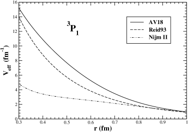
Figure 1: The comparison of three different effective strong potentials in the ${}^{3}P_{1}$ channel.

The meson-exchange effects, in the form of two-body exchange charges, give contributions of the form

$$d_{\mathcal{D}}^{(ex)}=\sqrt{\frac{1}{6}}\,\left(\langle\mathcal{D}||\int d^{3}x\,\rho^{(2)}(x)\,\bm{x}||\widetilde{\mathcal{D}}\rangle+\langle\mathcal{D}||\int d^{3}x\,\tilde{\rho}^{(2)}(x)\,\bm{x}||\mathcal{D}\rangle\right)\,,$$ (10)

where the first term corresponds to adding the normal ($P$- and $T$-even) exchange charge $\rho^{(2)}$ to Eq. (7), and the $\not{P}\not{T}$ exchange $\tilde{\rho}^{(2)}$, induced by $H_{\scriptscriptstyle{\not{P}\not{T}}}$, is included via the second term. Compared with the one-body charge, which is $\mathcal{O}(1)$, $\rho^{(2)}$ can be ignored since it gives a correction of $\mathcal{O}(1/m_{\scriptscriptstyle{N}})^{3}$ (see e.g. Ref. Riska (1989)). On the other hand, since $\tilde{\rho}^{(2)}$ can be as large as $\mathcal{O}(1/m_{\scriptscriptstyle{N}}^{2})$, and its contribution is evaluated within unperturbed deuteron wave functions, its significance should be investigated.

As indicated by the dominance of pion exchange observed above, and also in view of the suppression of heavy-meson exchange currents found in the study of the ($P$-odd, $T$-even) deuteron anapole moment Liu et al. (2003), the consideration of the pion sector is sufficient for the two-body exchange effects. Attaching a photon to every possible line in the one-pion exchange diagram which leads to $H_{\scriptscriptstyle{\not{P}\not{T}}}^{(\pi)}$, the exchange charge can then to $\mathcal{O}(1/m_{\scriptscriptstyle{N}}^{2})$ be identified, in configuration space, as

$$\tilde{\rho}_{pair}^{(\pi)}(\bm{x};\bm{r}_{1},\bm{r}_{2}) = \frac{e}{4\,m_{\scriptscriptstyle{N}}^{2}}\Big{(}(1+\kappa_{\scriptscriptstyle{S}})\,\big{(}\bar{G}_{\pi}^{(0)}\,\bm{\tau}_{1}\cdot\bm{\tau}_{2}+\bar{G}_{\pi}^{(1)}\,\tau_{1}^{z}+\bar{G}_{\pi}^{(2)}\,(3\,\tau_{1}^{z}\,\tau_{2}^{z}-\bm{\tau}_{1}\cdot\bm{\tau}_{2})\big{)}$$ (11)

$$+(1+\kappa_{\scriptscriptstyle{V}})\,(\bar{G}_{\pi}^{(0)}\,\tau_{2}^{z}+\bar{G}_{\pi}^{(1)}+2\,\bar{G}_{\pi}^{(2)}\,\tau_{2}^{z})\Big{)}\,\bm{\sigma}_{1}\cdot\bm{\nabla}_{x}\,\delta^{(3)}(\bm{x}-\bm{r}_{1})\,\mathcal{Y}_{\pi}(r)$$

$$+(1\leftrightarrow 2)\,,$$

$$\tilde{\rho}_{mesonic}^{(\pi)}(\bm{x};\bm{r}_{1},\bm{r}_{2}) = -\frac{e}{4\,m_{\scriptscriptstyle{N}}^{2}}\,i\,(\bm{\tau}_{1}\times\bm{\tau}_{2})^{z}\,(\bar{G}_{\pi}^{(0)}-\bar{G}_{\pi}^{(2)})\,(\bm{\sigma}_{1}\cdot\bm{\nabla}_{1}+\bm{\sigma}_{2}\cdot\bm{\nabla}_{2})$$ (12)

$$\times\big{[}\nabla_{1}^{2}-\nabla_{2}^{2}\,,\,\mathcal{Y}_{\pi}(r_{x1})\,\mathcal{Y}_{\pi}(r_{x2})\big{]}\,,$$

where the pair term refers to the diagram in which the photon couples to an intermediate nucleon-antinucleon pair and the mesonic term refers to the diagram in which the photon couples to the meson in flight; $r=|\bm{r}_{1}-\bm{r}_{2}|$, $r_{x1(2)}=|\bm{x}-\bm{r}_{1(2)}|$. Numerically, the contribution of these diagrams to the deuteron EDM is found to be

$$d_{\mathcal{D}}^{(ex)}\simeq 9.40\times 10^{-4}\,\bar{G}_{\pi}^{(1)}-5.28\times 10^{-4}\,\bar{G}_{\pi}^{(0)}\,.$$ (13)

Compared with $d_{\mathcal{D}}^{(pol)}$, this constitutes only a few-percent correction.

Combining the results for $d_{\mathcal{D}}^{(pol)}$ and $d_{\mathcal{D}}^{(ex)}$, we obtain for the two-body contribution to the deuteron EDM, in terms of $\not{P}\not{T}$ couplings,

$$d_{\mathcal{D}}^{(2)}=d_{\mathcal{D}}^{(pol)}+d_{\mathcal{D}}^{(ex)}\simeq 0.20\,\bar{g}_{\pi}^{(1)}+\mathcal{O}(\bar{g}_{\pi}^{(0)},\,\bar{g}_{\eta,\,\rho,\,\omega}^{(1)})\,,$$ (14)

with an error estimated as less than $5\%$.

Besides the usual exchange effects in which one of the meson-nucleon couplings is $P$- and $T$-odd, another class of diagrams involving a $\not{P}\not{T}$ photon coupling to the exchanged mesons can also contribute. Since pseudoscalar mesons cannot have such a $\not{P}\not{T}$ coupling to photons, the candidates in our current framework are $\not{P}\not{T}$ $\rho\pi\gamma$, $\omega\pi\gamma$, and $\rho\rho\gamma$ vertices. Assuming these $\not{P}\not{T}$ couplings are of the same order of magnitude, one can expect a smaller contribution from the $\rho\rho\gamma$ vertex, because the $\rho$ meson is much more massive and has a smaller strong coupling to nucleons than the pion. Therefore, in order to estimate the size of this type of contributions we evaluate the diagrams based on $\not{P}\not{T}$ $\rho\pi\gamma$ and $\omega\pi\gamma$ vertices shown in Fig. 2.

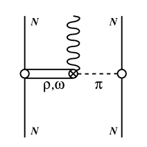
Figure 2: The two-body contribution to $d_{\mathcal{D}}$ arising from the first-order $\not{P}\not{T}$ $\rho$- and $\omega$-$\pi\gamma$ couplings.

Expressing the $\not{P}\not{T}$ $\rho\pi\gamma$ and $\omega\pi\gamma$ Lagrangian densities as

$$\mathcal{L}_{\scriptscriptstyle{\not{P}\not{T}}}^{(\rho\pi\gamma)} = \frac{e\,\bar{g}_{\rho\pi\gamma}}{2m_{\rho}}\,F^{\alpha\beta}\,\bm{\rho}_{\alpha}\cdot\partial_{\beta}\bm{\pi}\,,$$ (15)

$$\mathcal{L}_{\scriptscriptstyle{\not{P}\not{T}}}^{(\omega\pi\gamma)} = \frac{e\,\bar{g}_{\omega\pi\gamma}}{2m_{\omega}}\,F^{\alpha\beta}\,\omega_{\alpha}\,\partial_{\beta}\pi^{0}\,,$$ (16)

where two new $\not{P}\not{T}$ coupling constants $\bar{g}_{\rho\pi\gamma}$ and $\bar{g}_{\omega\pi\gamma}$ are introduced, the associated exchange charges are, in configuration space,

$$\tilde{\rho}_{mesonic}^{(\rho\pi\gamma^{\prime})}(\bm{x};\bm{r}_{1},\bm{r}_{2}) = \frac{eg_{\rho\scriptscriptstyle{NN}}g_{\pi\scriptscriptstyle{NN}}\bar{g}_{\rho\pi\gamma}}{4m_{\rho}m_{\scriptscriptstyle{N}}}\,\bm{\tau}_{1}\cdot\bm{\tau}_{2}\,(\bm{\nabla}\cdot\bm{\nabla}_{2})(\bm{\sigma}_{2}\cdot\bm{\nabla}_{2})\,\mathcal{Y}_{\rho}(r_{x1})\mathcal{Y}_{\pi}(r_{x2})+(1\leftrightarrow 2)\,,$$ (17)

$$\tilde{\rho}_{mesonic}^{(\omega\pi\gamma^{\prime})}(\bm{x};\bm{r}_{1},\bm{r}_{2}) = \frac{eg_{\omega\scriptscriptstyle{NN}}g_{\pi\scriptscriptstyle{NN}}\bar{g}_{\omega\pi\gamma}}{4m_{\omega}m_{\scriptscriptstyle{N}}}\,(\bm{\nabla}\cdot\bm{\nabla}_{2})(\bm{\sigma}_{2}\cdot\bm{\nabla}_{2})\,\mathcal{Y}_{\omega}(r_{x1})\mathcal{Y}_{\pi}(r_{x2})+(1\leftrightarrow 2)\,.$$ (18)

The numerical calculation, using the A$v_{18}$ potential, gives an EDM contribution of about $2.3\times 10^{-3}\,(\bar{g}_{\rho\pi\gamma}-\bar{g}_{\omega\pi\gamma})$. Since the coefficient is two orders of magnitude smaller than the leading coefficient of $\bar{g}_{\pi}^{(1)}$ in Eq. (14), we shall ignore these mesonic $\not{P}\not{T}$ effects for the rest of this work.

III.2 One-Body Contributions

The total one-body contribution to the deuteron EDM is simply the sum of the proton and neutron EDMs, i.e.

$$d_{\mathcal{D}}^{(1)}=d_{p}+d_{n}\,.$$ (19)

Our goal in this section is to evaluate $d_{p}$ and $d_{n}$ in a manner consistent with the framework used for the $\not{P}\not{T}$ $N\!N$ interaction.

The nucleon EDM has a wide variety of sources such as the QCD $\bar{\theta}$ term, quark EDMs and chromo-EDMs (CEDMs), Weinberg three-gluon operator, and four-quark contact interactions, therefore, its evaluation requires good knowledge of nonperturbative dynamics of confined quarks, which is still not available. A commonly used method of estimate is to evaluate the hadronic loop diagrams, in which meson and baryon degrees of freedom are used to describe the dynamics and the dependence on the $\not{P}\not{T}$ mechanisms at the quark-gluon level is subsumed in the $\not{P}\not{T}$ meson-nucleon coupling constants. This approach has been applied extensively to the neutron EDM in various contexts (see, for example, Refs. Barton and White (1969); Crewther et al. (1979); McKellar et al. (1987); He et al. (1989); Valencia (1990); Pich and de Rafael (1991); Khatsymovsky and Khriplovich (1992); Khriplovich and Zyablyuk (1996); Borasoy (2000)). Here we apply it to both the proton and the neutron EDM, with the inclusion of vector mesons.

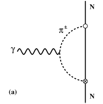
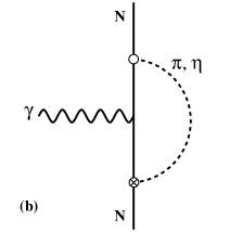
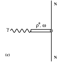
Figure 3: Hadronic loop diagrams which contribute to the nucleon EDM.

The loop diagrams containing a virtual pseudoscalar meson are classified as in Fig. 3(a) and Fig. 3(b), where the photon couples to the charged pseudoscalar meson in the former and to the intermediate nucleon in the latter case. Defining the hadronic loop contribution to the nucleon EDM as

$$d_{\scriptscriptstyle{N}}^{(had)}\equiv\frac{e}{4\pi^{2}m_{\scriptscriptstyle{N}}}\left(\delta_{\scriptscriptstyle{S}}\,\frac{1}{2}+\delta_{\scriptscriptstyle{V}}\,\frac{\tau^{z}}{2}\right)\,,$$ (20)

the results for the corresponding diagrams are

$$\delta_{\scriptscriptstyle{S}}^{(a)} = 0\,,$$ (21)

$$\delta_{\scriptscriptstyle{V}}^{(a)} = -2(\bar{G}_{\pi}^{(0)}-\bar{G}_{\pi}^{(2)})\mathcal{I}_{0}^{(\pi)}\,,$$ (22)

$$\delta_{\scriptscriptstyle{S}}^{(b)} = (3\bar{G}_{\pi}^{(0)}+\bar{G}_{\pi}^{(1)})\mathcal{I}_{1}^{(\pi)}-(3\kappa_{\scriptscriptstyle{S}}\bar{G}_{\pi}^{(0)}+\kappa_{\scriptscriptstyle{V}}\bar{G}_{\pi}^{(1)})\mathcal{I}_{2}^{(\pi)}$$ (23)

$$+(\bar{G}_{\eta}^{(0)}+\bar{G}_{\eta}^{(1)})\mathcal{I}_{1}^{(\eta)}-(\kappa_{\scriptscriptstyle{S}}\bar{G}_{\eta}^{(0)}+\kappa_{\scriptscriptstyle{V}}\bar{G}_{\eta}^{(1)})\mathcal{I}_{2}^{(\eta)}\,,$$

$$\delta_{\scriptscriptstyle{V}}^{(b)} = (-\bar{G}_{\pi}^{(0)}+\bar{G}_{\pi}^{(1)}+4\bar{G}_{\pi}^{(2)})\mathcal{I}_{1}^{(\pi)}-(-\kappa_{\scriptscriptstyle{V}}\bar{G}_{\pi}^{(0)}+\kappa_{\scriptscriptstyle{S}}\bar{G}_{\pi}^{(1)}+4\kappa_{\scriptscriptstyle{V}}\bar{G}_{\pi}^{(2)})\mathcal{I}_{2}^{(\pi)}$$ (24)

$$+(\bar{G}_{\eta}^{(0)}+\bar{G}_{\eta}^{(1)})\mathcal{I}_{1}^{(\eta)}-(\kappa_{\scriptscriptstyle{V}}\bar{G}_{\eta}^{(0)}+\kappa_{\scriptscriptstyle{S}}\bar{G}_{\eta}^{(1)})\mathcal{I}_{2}^{(\eta)}\,.$$

The three distinct loop integrals involving an $i$-type pseudoscalar meson, $\mathcal{I}_{0}^{(i)}$, $\mathcal{I}_{1}^{(i)}$, and $\mathcal{I}_{2}^{(i)}$, correspond to the cases where the photon couples to the pseudoscalar meson, the nucleon Dirac, and the nucleon Pauli form factor, respectively. They are evaluated as

$$\mathcal{I}_{0}^{(i)} = -1-(1-x_{i}^{2})\,\ln x_{i}+x_{i}^{2}\,(3-x_{i}^{2})\,\mathcal{F}(x_{i}^{2})$$ (25)

$$\xrightarrow[x_{i}\ll 1]{} -\ln x_{i}-1+\frac{3\,\pi}{4}\,x_{i}+x_{i}^{2}\,\ln x_{i}+\mathcal{O}(x_{i}^{2})\,,$$

$$\mathcal{I}_{1}^{(i)} = \frac{1}{2}-\frac{1}{2}\,x_{i}^{2}\,\ln x_{i}-x_{i}^{2}\,(1-\frac{1}{2}x_{i}^{2})\,\mathcal{F}(x_{i}^{2})$$ (26)

$$\xrightarrow[x_{i}\ll 1]{} \frac{1}{2}-\frac{\pi}{4}\,x_{i}-\frac{1}{2}\,x_{i}^{2}\,\ln x_{i}+\mathcal{O}(x_{i}^{2})\,,$$

$$\mathcal{I}_{2}^{(i)} = \frac{11}{16}+\frac{3}{8}\,x_{i}^{2}-\frac{1}{16}\,x_{i}^{2}\,(1+3\,x_{i}^{2})\,\ln x_{i}-x_{i}^{2}\,(1+\frac{5}{8}\,x_{i}^{2}+\frac{3}{8}\,x_{i}^{2})\,\mathcal{F}(x_{i}^{2})$$ (27)

$$\xrightarrow[x_{i}\ll 1]{} \frac{11}{16}-\frac{\pi}{4}\,x_{i}-\frac{1}{8}x_{i}^{2}\,\ln x_{i}+\mathcal{O}(x_{i}^{2})\,,$$

$$\mathcal{F}(s) = \frac{1}{\sqrt{4\,s+s^{2}}}\left(\tan^{-1}\left[\frac{2-s}{\sqrt{4\,s+s^{2}}}\right]+\tan^{-1}\left[\frac{s}{\sqrt{4\,s+s^{2}}}\right]\right)\,,$$ (28)

where $x_{i}=m_{i}/m_{\scriptscriptstyle{N}}$. Since both meson and nucleon form factors were taken to be constant off the mass shell, and since form factors fall off as the square of the four-momentum transfer increases, these results should be viewed as an upper bound McKellar et al. (1987).

From Eqs. (25)–(27), one observes that only $\mathcal{I}_{0}^{(\pi)}$ has a non-analytic term, i.e. $\ln x_{\pi}$, in the chiral limit, $m_{\pi}\rightarrow 0$. The mathematical reason is that Fig. 3(a) contains more pion propagators than Fig. 3(b), which is responsible for the infrared divergence in the soft-pion limit Crewther et al. (1979). Therefore, the contribution to the nucleon EDM involving chiral logarithms is purely isovector,

$$d_{\scriptscriptstyle{N}}^{(\pi)}=-\frac{e\tau^{z}}{4\pi^{2}m_{\scriptscriptstyle{N}}}\,(\bar{G}_{\pi}^{(0)}-\bar{G}_{\pi}^{(2)})\ln\left(\frac{m_{N}}{m_{\pi}}\right)\,.$$ (29)

This implies that the deuteron EDM receives no one-body contribution from loop diagrams involving $\pi$ and $\eta$ mesons in the chiral limit. Furthermore, when the neutron EDM is considered, the constant terms in $\mathcal{I}_{0}$ and $\mathcal{I}_{1}$ exactly cancel, as has been pointed out in Ref. Pich and de Rafael (1991). However, this is not true for the proton.

Because chiral symmetry is explicitly broken by the pion mass, it is interesting to compare the chiral logarithm with other, analytic, terms when realistic parameters are used. For example, taking $x_{\pi}=140/940$ in Eq. (25), one gets $\mathcal{I}_{0}^{(\pi)}\simeq 1.19$, which is about $40\%$ smaller than $-\ln(m_{\pi}/m_{\scriptscriptstyle{N}})\simeq 1.90$. This sizable difference typically sets the scale for the theoretical uncertainty. The same conclusion can be drawn from the work by Barton and White Barton and White (1969) who, motivated by the success of sideways dispersion relations for the nucleon Pauli form factors Drell and Pagels (1965), applied the same technique with the same parameters to the neutron EDM problem. This analysis, involving mainly the threshold pion-photoproduction amplitude, is actually similar to the evaluation of type (a) loop diagram with soft pions, and in fact produces the same chiral logarithm. Compared with the leading term which gave $d_{n}\simeq 0.8\times 10^{-11}$ $e$–fm (a value, in our notation, $\bar{g}_{\pi}^{(0)}-\bar{g}_{\pi}^{(2)}=1.2\times 10^{-10}$ was used as input), their full analysis predicted $d_{n}\simeq 0.5\times 10^{-11}$ $e$–fm, which is also some $40\%$ smaller. While this may be just an accident, it does signal a potentially large theoretical uncertainty for the nucleon EDM.

In order to estimate the relevance of the vector-meson degrees of freedom to the nucleon EDM, we consider the diagrams illustrated in Fig. 3(c). These contributions can be roughly estimated by the assumption of VMD, which leads to a dispersion-theory analysis of the $\rho^{0}$ and $\omega$ poles in the time-like region. The deuteron is only sensitive to the isoscalar sector, for which, in the case of the nucleon Pauli form factor, the naive VMD model works rather well. The vector-meson contributions to the isovector nucleon EDM should, however, also be added as a correction to the leading result from the pion-loop calculation, which is equivalent to including the $2\pi$ continuum in the dispersion-theory analysis.

The required vector-meson-photon conversion mechanism is introduced by the Lagrangian density

$$\mathcal{L}_{\scriptscriptstyle{\mathrm{VMD}}}=\frac{e}{2f_{\rho}}F^{\mu\nu}F_{\mu\nu}^{(\rho)}+\frac{e}{2f_{\omega}}F^{\mu\nu}F_{\mu\nu}^{(\omega)}\,,$$ (30)

where the $F^{\mu\nu}$’s denote the field tensors for the photon and the $\rho^{0}$ and $\omega$ mesons; the constants $f_{\rho}=5.00$ and $f_{\omega}=17.05$ are determined from the decay widths $\Gamma_{\rho,\omega\rightarrow e^{+}e^{-}}=6.85,0.60$ MeV Hagiwara et al. (2002) by $\Gamma_{x\rightarrow e^{+}e^{-}}=4\pi\alpha^{2}m_{\scriptscriptstyle{N}}/(3f_{x}^{2})$. Then the vector-meson contributions to the nucleon EDM are evaluated as

$$\delta_{\scriptscriptstyle{S}}^{(c)} = \frac{4\pi^{2}}{f_{\rho}g_{\rho\scriptscriptstyle{NN}}}\bar{G}_{\rho}^{(1)}+\frac{4\pi^{2}}{f_{\omega}g_{\omega\scriptscriptstyle{NN}}}\bar{G}_{\omega}^{(0)}\,,$$ (31)

$$\delta_{\scriptscriptstyle{V}}^{(c)} = \frac{4\pi^{2}}{f_{\rho}g_{\rho\scriptscriptstyle{NN}}}(\bar{G}_{\rho}^{(0)}+2\bar{G}_{\rho}^{2})+\frac{4\pi^{2}}{f_{\omega}g_{\omega\scriptscriptstyle{NN}}}\bar{G}_{\omega}^{(1)}\,.$$ (32)

Keeping in mind the caveat of a possibly large theoretical error, we nevertheless take a more adventurous point of view and include also the analytic terms in $\mathcal{I}_{0}$ and $\mathcal{I}_{1}$, i.e. $\mathcal{I}_{0}^{(\pi)}\simeq 1.19$, $\mathcal{I}_{1}^{(\pi)}\simeq 0.41$, and $\mathcal{I}_{1}^{(\eta)}\simeq 0.28$, but we neglect the part from the nucleon Pauli form factor, so we set $\mathcal{I}_{2}^{(\pi)}=\mathcal{I}_{2}^{(\eta)}=0$. Collecting the results from Eqs. (20), (21)–(24), (31)–(32), the total one-body contribution to the deuteron EDM is evaluated as

$$d_{\mathcal{D}}^{(1)} = 2.18\times 10^{-3}\,(3\,\bar{G}_{\pi}^{(0)}+\bar{G}_{\pi}^{(1)})+1.49\times 10^{-3}\,(\bar{G}_{\eta}^{(0)}+\bar{G}_{\eta}^{(1)})$$ (33)

$$+1.53\times 10^{-2}\,\bar{G}_{\rho}^{(1)}+1.49\times 10^{-3}\,\bar{G}_{\omega}^{(0)}\,.$$

In terms of the $\not{P}\not{T}$ meson-nucleon coupling constants, the result is

$$d_{\mathcal{D}}^{(1)}=0.03\,\bar{g}_{\pi}^{(1)}+0.09\,\bar{g}_{\pi}^{(0)}+0.04\,\bar{g}_{\rho}^{(1)}+0.01\,\bar{g}_{\omega}^{(0)}+\mathcal{O}(\bar{g}_{\eta}^{(0,1)})\,.$$ (34)

IV Discussion

Combining Eqs. (14) and (34), we arrive at our final estimate for the deuteron EDM:

$$d_{\mathcal{D}}=(0.20+0.03)\,\bar{g}_{\pi}^{(1)}+0.09\,\bar{g}_{\pi}^{(0)}+0.04\,\bar{g}_{\rho}^{(1)}+0.01\,\bar{g}_{\omega}^{(0)}\,.$$ (35)

while our results at the same time imply the following predictions for the proton and neutron EDMs:

$$d_{p} = -0.08(\bar{g}_{\pi}^{(0)}-\bar{g}_{\pi}^{(2)})+0.03(\bar{g}_{\pi}^{(0)}+\bar{g}_{\pi}^{(1)}+2\bar{g}_{\pi}^{(2)})+3\times 10^{-3}(\bar{g}_{\eta}^{(0)}+\bar{g}_{\eta}^{(1)})$$

$$+0.02(\bar{g}_{\rho}^{(0)}+\bar{g}_{\rho}^{(1)}+2\bar{g}_{\rho}^{(2)})+6\times 10^{-3}(\bar{g}_{\omega}^{(0)}+\bar{g}_{\omega}^{(1)})\,,$$

$$d_{n} = 0.14(\bar{g}_{\pi}^{(0)}-\bar{g}_{\pi}^{(2)})-0.02(\bar{g}_{\rho}^{(0)}-\bar{g}_{\rho}^{(1)}+2\bar{g}_{\rho}^{(2)})+6\times 10^{-3}(\bar{g}_{\omega}^{(0)}-\bar{g}_{\omega}^{(1)})\,.$$ (37)

The leading contribution to $d_{\mathcal{D}}$, $0.20\,\bar{g}_{\pi}^{(1)}$, due to the $\not{P}\not{T}$ $N\!N$ interaction, including the exchange charges and calculated by using state-of-the-art wave functions, is $25\%$ smaller than the result assuming the zero-range approximation Khriplovich and Korkin (2000) which was adopted for an analysis on $C\!P$ violation models in Ref. Lebedev et al. (2004). The remaining contributions come from the proton and neutron EDMs. These terms have a sizable theoretical uncertainty, which could be as large as $40\%$. The non-vanishing dependence on $\bar{g}_{\pi}^{(0)}$, which arises from including analytic terms in the hadronic loop calculations, sets the stage for the QCD $\bar{\theta}$ term to play a role in the deuteron. Using the prediction by Crewther et al. Crewther et al. (1979) that $\bar{g}_{\pi}^{(0)}\simeq 0.027\bar{\theta}$, one gets a $d_{\mathcal{D}}\sim 2\times 10^{-3}\bar{\theta}$ dependence on $\bar{\theta}$, which is about three times larger than the QCD sum-rule calculation Pospelov and Ritz (1999); Lebedev et al. (2004). The dependence on the vector-meson couplings, though suppressed at the two-body level, enter the final result through the nucleon EDM where it could be sizable. An important issue in this respect is the size of the $\not{P}\not{T}$ $\rho$, $\omega$ (and $\eta$ for that matter) coupling constants compared to those of the pion. An argument by Gudkov et al. suggested that these vector-meson coupling constants are less significant Gudkov et al. (1993), while a recent work by Pospelov based on QCD sum rules gave the “best” values for $\bar{g}_{\rho,\omega}$ of the same order of magnitude as $\bar{g}_{\pi}$ Pospelov (2002); and these two works surprisingly have opposite predictions about the relative importance of $\bar{g}_{\pi^{\pm}}/\bar{g}_{\pi^{0}}$. Furthermore, work on the $P$-odd, $T$-even $N\!N$ interaction implied vector couplings at least equally important and preferably larger than their pseudoscalar counterparts (see e.g. Refs. Desplanques et al. (1980); Haxton et al. (2001, 2002)). Therefore, until consensus is reached, these vector-meson contributions should still be kept for maintaining a greater generality.

In order to connect expression Eq. (35) for the deuteron EDM to the underlying $C\!P$ violation, the $\not{P}\not{T}$ meson-nucleon coupling constants have to be expressed in terms of parameters at particle-physics level, such as the QCD $\bar{\theta}$ term, quark EDMs and CEDMs, etc. These quantities have a plethora of predictions from extensions of the Standard Model. Because all the EDM measurements to date only resulted in upper bounds, it is a popular practice to use these experimental limits to derive the corresponding bounds for one particular source of $C\!P$ violation while turning other possibilities off in an ad hoc fashion. Even though this simplification is legitimate to some extent, one might obtain an overconstraint by excluding possible cancellations between various $C\!P$-violation sources.

The deuteron and neutron results illustrate how limits on their EDMs could be used to provide tight constraints on a specific model of $C\!P$ violation, such as the one in Ref. Pospelov (2002). For supersymmetric models in which the Pecci-Quinn symmetry is evoked to remove the QCD $\bar{\theta}$ term, the quark CEDMs are the dominant contributors to the $\not{P}\not{T}$ meson-nucleon coupling constants, compared to the three-gluon and four-quark operators. Therefore, all the $\bar{g}$’s can be expressed in terms of the $d_{q}^{c}$’s. Using the “best” values recommended in Ref. Pospelov (2002): $\bar{g}_{\pi}^{(1)}\simeq 20\,d_{-}^{c}$, $\bar{g}_{\pi}^{(0)}\simeq 4\,d_{+}^{c}$, $\bar{g}_{\rho}^{(0)}\simeq 13.3\,d_{+}^{c}$, $\bar{g}_{\rho}^{(1)}\simeq-8.6\,d_{-}^{c}$, $\bar{g}_{\omega}^{(0)}\simeq-8.6\,d_{+}^{c}$, $\bar{g}_{\omega}^{(1)}\simeq-13.3\,d_{-}^{c}$, where $d_{\pm}^{c}=d_{u}^{c}\pm d_{d}^{c}$, the deuteron and neutron EDMs can be completely expressed in terms of the CEDMs of the up and down quarks, viz.

$$d_{\mathcal{D}} = -4.67\,d_{d}^{c}+5.22\,d_{u}^{c}\,,$$ (38)

$$d_{n} = -0.01\,d_{d}^{c}+0.49\,d_{u}^{c}\,.$$ (39)

Thus, these two EDM measurements probe different linear combinations of $d_{d}^{c}$ and $d_{u}^{c}$ in this case. Moreover, the deuteron could be significantly more sensitive than the neutron. This example is clearly oversimplified, however, judging from the general expressions Eqs. (35) and (37), one expects that, barring unnatural and accidental cancellations, the deuteron is competitive to the neutron in sensitivity to $C\!P$ violation. Furthermore, the deuteron EDM involves different $\not{P}\not{T}$ coupling constants, and hence in general will be complementary with respect to the information about $C\!P$ violation that can be probed with the neutron.

In conclusion, it should be realized that the theoretical uncertainties, especially in the results for $d_{p}$ and $d_{n}$ and hence in the one-body contribution to $d_{\mathcal{D}}$, are significant. The calculation of an atomic or nuclear EDM involves a broad range of physics, including the problematic strong interaction at the nuclear and subnuclear scale. In this respect, it is relevant that efforts have been renewed recently to attack the neutron EDM in lattice QCD Guadagnoli et al. (2003). In general, improved treatments of the hadronic physics, which can bridge the phenomenology of the neutron EDM and $\not{P}\not{T}$ nuclear forces with the underlying particle physics, are of central interest.

Appendix A Deuteron MQM

Besides the EDM, the $\not{P}\not{T}$ $N\!N$ interaction can also induce $P$- and $T$-odd electromagnetic moments of higher multipolarity, that is, $C3$, $C5$, and $M2$, $M4$, etc. For a spin-1 object such as the deuteron, a nonzero $M2$ magnetic quadrupole moment (MQM) is therefore another signature of $C\!P$ violation. Approximating the nuclear electromagnetic current as purely one-body, i.e. ignoring the meson-exchange currents, the MQM operator can be expressed, in a Cartesian basis, as

$$M_{mn}=\frac{e}{2m_{\scriptscriptstyle{N}}}\left\{\mu\left[3\,r_{m}\,\sigma_{n}+3\,r_{n}\,\sigma_{m}-2\,\bm{\sigma}\cdot\bm{r}\,\delta_{mn}\right]+2\,q\left(r_{m}\,L_{n}+r_{n}\,L_{m}\right)\right\}\,,$$ (40)

where $\mu$, $q$, and $L$ denote the nucleon magnetic moment, charge (in uints of $e$), and orbital angular momentum, respectively Khriplovich and Korkin (2000). The deuteron MQM, defined by

$$M_{\mathcal{D}}=2\langle\mathcal{D},J_{z}=1|\sum_{i=1}^{2}M_{zz}(i)|\widetilde{{\mathcal{D}}},J_{z}=1\rangle\,,$$ (41)

can then be evaluated once the ${}^{1}P_{1}$ and ${}^{3}P_{1}$ parity admixtures have been calculated. Assuming $\not{P}\not{T}$ one-pion exchange only, and using the A$v_{18}$ strong potential gives the numerical result

$$M_{\mathcal{D}}=0.051\,\mu_{\scriptscriptstyle{S}}\,\bar{g}_{\pi}^{(0)}+(0.031\,\mu_{\scriptscriptstyle{V}}+0.003)\,\bar{g}_{\pi}^{(1)}\,,$$ (42)

in units of $e$–fm². The model-dependency is at the $1\%$ level, similar to the EDM calculation.

Although the isoscalar spin current leads to a rather large matrix element (in the zero-range approximation of Ref. Khriplovich and Korkin (2000), it is three times the isovector one), the isoscalar magnetic moment renders the resulting $\bar{g}_{\pi}^{(0)}$ coefficient, 0.04, smaller than the $\bar{g}_{\pi}^{(1)}$ coefficient, 0.15, which is dominated by the isovector spin current from the large isovector magnetic moment. The orbital motion adds only a small correction to the $\bar{g}_{\pi}^{(1)}$ term through the deuteron $D$-wave component.

While a sensitive experiment to measure $M_{\mathcal{D}}$ appears as least as formidable as for $d_{\mathcal{D}}$, it might be contemplated with deuterium atoms, because the MQM, unlike the EDM, is not screened by the electron. An interesting theoretical point is that, since the nucleon itself has no quadrupole moment, the deuteron MQM is a rather clean probe of the $\not{P}\not{T}$ $N\!N$ interaction, and in particular of $\bar{g}_{\pi}^{(1)}$.

References

• Khriplovich and Lamoreaux (1997) I. B. Khriplovich and S. K. Lamoreaux, CP Violation Without Strangeness: Electric Dipole Moments of Particles, Atoms, and Molecules (Springer Verlag, Berlin, 1997).
• Barr (1993) S. M. Barr, Int. J. Mod. Phys. A 8, 209 (1993).
• Ramsey (1990) N. F. Ramsey, Annu. Rev. Nucl. Part. Sci. 40, 1 (1990).
• Harris et al. (1999) P. G. Harris et al., Phys. Rev. Lett. 82, 904 (1999).
• Sandars (2001) P. G. H. Sandars, Contemp. Phys. 42, 97 (2001).
• Romalis et al. (2001) M. V. Romalis, W. C. Griffith, J. P. Jacobs, and E. N. Fortson, Phys. Rev. Lett. 86, 2505 (2001).
• Purcell and Ramsey (1950) E. M. Purcell and N. F. Ramsey, Phys. Rev. 78, 807 (1950).
• Schiff (1963) L. I. Schiff, Phys. Rev. 132 (1963).
• Engel et al. (2000) J. Engel, J. L. Friar, and A. C. Hayes, Phys. Rev. C 61, 035502 (2000).
• Semertzidis et al. (2004) Y. K. Semertzidis et al., AIP Conf. Proc. 698, 200 (2004).
• Farley et al. (2003) F. J. M. Farley et al. (2003), accepted for publication in Phys. Rev. Lett, eprint hep-ex/0307006.
• Onderwater and Semertzidis (private communication) C. J. G. Onderwater and Y. K. Semertzidis (private communication).
• de Swart et al. (1995) J. J. de Swart, C. P. F. Terheggen, and V. G. J. Stoks (1995), eprint nucl-th/9509032.
• Fischler et al. (1992) W. Fischler, S. Paban, and S. Thomas, Phys. Lett. B289, 373 (1992).
• Herczeg (1966) P. Herczeg, Nucl. Phys. 75, 655 (1966).
• Barton (1961) G. Barton, Nuovo Cim. 19, 512 (1961).
• Haxton and Henley (1983) W. C. Haxton and E. M. Henley, Phys. Rev. Lett. 51, 1937 (1983).
• Herczeg (1987) P. Herczeg, in Tests of Time Reversal Invariance in Neutron Physics, edited by N. R. Roberson, C. R. Gould, and J. D. Bowman (World Scientific, Singapore, 1987), pp. 24–53.
• Gudkov et al. (1993) V. P. Gudkov, X.-G. He, and B. H. J. McKellar, Phys. Rev. C 47, 2365 (1993).
• Towner and Hayes (1994) I. S. Towner and A. C. Hayes, Phys. Rev. C 49, 2391 (1994).
• Stoks et al. (1993) V. Stoks, R. Timmermans, and J. J. de Swart, Phys. Rev. C 47, 512 (1993).
• Rentmeester et al. (1999) M. C. M. Rentmeester, R. G. E. Timmermans, J. L. Friar, and J. J. de Swart, Phys. Rev. Lett. 82, 4992 (1999).
• Tiator et al. (1994) L. Tiator, C. Bennhold, and S. S. Kamalov, Nucl. Phys. A580, 455 (1994).
• Höhler and Pietarinen (1975) G. Höhler and E. Pietarinen, Nucl. Phys. B95, 210 (1975).
• de Swart et al. (1994) J. J. de Swart, P. M. M. Maessen, and T. A. Rijken, in Properties and Interactions of Hyperons, edited by B. F. Gibson, P. D. Barnes, and K. Nakai (World Scientific, 1994), pp. 37–54.
• Sakurai (1969) J. J. Sakurai, Currents and Mesons (University of Chicago Press, Chicago, 1969).
• Wiringa et al. (1995) R. B. Wiringa, V. G. J. Stoks, and R. Schiavilla, Phys. Rev. C 51, 38 (1995).
• Stoks et al. (1994) V. G. J. Stoks, R. A. M. Klomp, C. P. F. Terheggen, and J. J. de Swart, Phys. Rev. C 49, 2950 (1994).
• Avishai (1985) Y. Avishai, Phys. Rev. D 32, 314 (1985).
• Khriplovich and Korkin (2000) I. B. Khriplovich and R. A. Korkin, Nucl. Phys. A665, 365 (2000).
• Riska (1989) D. O. Riska, Phys. Rep. 181, 207 (1989).
• Liu et al. (2003) C.-P. Liu, C. H. Hyun, and B. Desplanques, Phys. Rev. C 68, 045501 (2003).
• Barton and White (1969) G. Barton and E. D. White, Phys. Rev. 184, 1660 (1969).
• Crewther et al. (1979) R. J. Crewther, P. Di Vecchia, G. Veneziano, and E. Witten, Phys. Lett. B88, 123 (1979), ibid. 91, 487(E) (1980).
• McKellar et al. (1987) B. H. J. McKellar, S. R. Choudhury, X.-G. He, and S. Pakvasa, Phys. Lett. B197, 556 (1987).
• He et al. (1989) X.-G. He, B. H. J. McKellar, and S. Pakvasa, Int. J. Mod. Phys. A 4, 5011 (1989), ibid. 6, 1063(E) (1991).
• Valencia (1990) G. Valencia, Phys. Rev. D 41, 1562 (1990).
• Pich and de Rafael (1991) A. Pich and E. de Rafael, Nucl. Phys. B367, 313 (1991).
• Khatsymovsky and Khriplovich (1992) V. M. Khatsymovsky and I. B. Khriplovich, Phys. Lett. B296, 219 (1992).
• Khriplovich and Zyablyuk (1996) I. B. Khriplovich and K. N. Zyablyuk, Phys. Lett. B383, 429 (1996).
• Borasoy (2000) B. Borasoy, Phys. Rev. D 61, 114017 (2000).
• Drell and Pagels (1965) S. D. Drell and H. R. Pagels, Phys. Rev. 140, B397 (1965).
• Hagiwara et al. (2002) K. Hagiwara et al., Phys. Rev. D 66, 010001 (2002).
• Lebedev et al. (2004) O. Lebedev, K. A. Olive, M. Pospelov, and A. Ritz (2004), eprint hep-ph/0402023.
• Pospelov and Ritz (1999) M. Pospelov and A. Ritz, Phys. Rev. Lett. 83, 2526 (1999).
• Pospelov (2002) M. Pospelov, Phys. Lett. B530, 123 (2002).
• Desplanques et al. (1980) B. Desplanques, J. F. Donoghue, and B. R. Holstein, Ann. Phys. 124, 449 (1980).
• Haxton et al. (2001) W. C. Haxton, C.-P. Liu, and M. J. Ramsey-Musolf, Phys. Rev. Lett. 86, 5247 (2001).
• Haxton et al. (2002) W. C. Haxton, C.-P. Liu, and M. J. Ramsey-Musolf, Phys. Rev. C 65, 045502 (2002).
• Pospelov (private communication) M. Pospelov (private communication).
• Guadagnoli et al. (2003) D. Guadagnoli, V. Lubicz, G. Martinelli, and S. Simula, J. High Energy Phys. 04, 019 (2003).