Testing Non-local Nucleon-Nucleon Interactions in the Four-Nucleon Systems

Abstract

The Faddeev-Yakubovski equations are solved in configuration space for the $\alpha$-particle and n-³H continuum states. We test the ability of nonlocal nucleon-nucleon interaction models to describe 3N and 4N systems.

I Introduction

In a fundamental description of nucleon-nucleon (NN) interaction, the existence of the nucleon internal structure can not be ignored. The standard NN potentials are actually effective tools aiming to mimic a much more complicated interaction process, of which it is not even clear that it could be reduced to a potential problem. The NN system can be rigorously described only when starting from the underlying QCD theory for the nucleon constituents: quarks and gluons. This is however a very difficult task, which is just becoming accessible in lattice calculations BBPS_PLB585 ; Beane_FB17_03 ; WPWG , and that will be in any case limited for a long time to the two-nucleon system. In any attempt to describe the nuclear structure, one is thus obliged to rely on more or less phenomenological models.

Since the nucleon size is comparable to the strong interaction range, the effects of its internal structure are expected to be considerable. In particular the NN interaction should be non-local, at least for small inter-nucleon distances. In addition, we have no reason to believe that nuclear interaction is additive as the Coulomb one: the interaction between two nucleons may not be independent of the presence of a third one in their vicinity. Finally the interplay of nucleon confinement and relatively large kinetic energies can generate – e.g. via virtual nucleon excitations – a rather strong energy-dependence in the interaction. Despite numerous studies devoted to this subject, we still do not have a clear understanding of the relative importance of these effects in NN force, specially concerning their influence on experimentally measurable quantities.

This work investigates the consequences of using non-local NN forces in describing the A=3 and A=4 nuclear systems. The locality of NN force, assumed in some of the so called realistic models AV18_PRC_95 ; NIJ_PRC49_94 , is due more to numerical convenience than to convincing physical arguments. The two-nucleon experimental data, since they contain only on-shell physics, are successfully reproduced without including any energy dependence or non-locality in the NN force. However, they all suffer from the underbinding problem, i.e. two-nucleon interaction alone fails to reproduce the nuclear binding energies, starting already from the simplest A=3 nuclei. Figure 1 shows the relative differences between experimental and theoretical binding energies for He isotopes obtained with AV18 potential AV18_PRC_95 ; PPWC_PRC64_01 ; PVW_PRC66_02 . These differences increase with the mass number A and vary from $\sim 0.7$ MeV in ³He to $\sim 10$ MeV in the case of ¹⁰He.

The inclusion of non-local terms – like in Nijm 93 and Nijm I potentials NIJ_PRC49_94 – does not remove this discrepancy FPSdS_93 ; Nogga_alp . If in some cases, like in CD-Bonn CD_Bonn or in chiral models EM_PLB524_02 ; EGM_NPA637_98 ; EGM_NPA671_00 , they considerably improve 3- and 4-N binding energies, the improvement is still not sufficient to reproduce the experimental values. This underbinding is rather easily removed by means of three-nucleon forces (3NF). The existence of such forces is doubtless, but their strength depends on the NN partner in use and is determined only by fitting requirements.

However the use of 3NF, to some extent, can be just a matter of taste. It has been shown in GP_FBS9_90 ; Polyzou_PRC58_98 that two different, but phase-equivalent, two-body interactions are related by a unitary, non-local, transformation. One thus could expect that a substantial part of 3- and multi-nucleon forces could also be absorbed by non local terms. A considerable simplification would result if the bulk of experimental data could be described by only using two-body non-local interaction. In fact, the unique aim of any phenomenological model is to provide a satisfactory description of the experimental observables but it is worth reaching this aim by using the simplest possible approach.

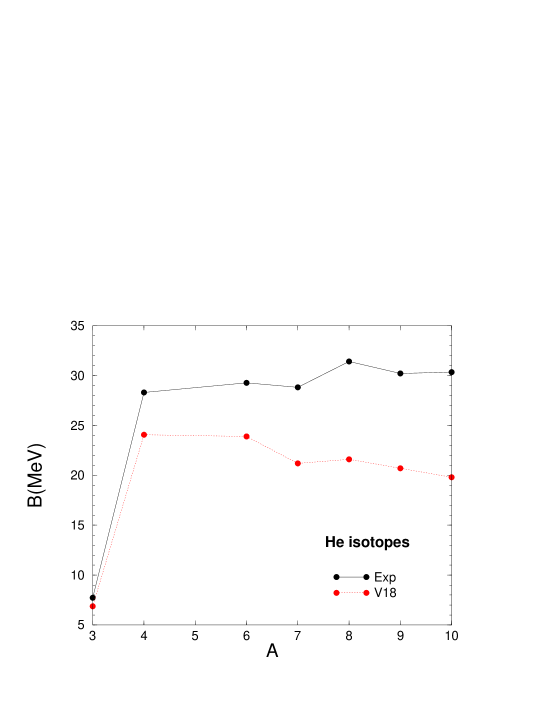
Figure 1: ”(Color online)” Comparison between the experimental and theoretical calculations with Argonne v18 interaction in He isotopes. Results are taken from PPWC_PRC64_01 ; PVW_PRC66_02 .

There exist already calculations reproducing the triton binding energy without making explicit use of 3NF. The first one was obtained by Gross and Stadler Gross using a relativistic equation and benefiting from some additional freedom in the off-shell vertex form factors. The complexity in using relativistic equations makes however difficult their extension to larger nuclear systems, or even to 3N scattering.

A very promising result, which takes profit from non-locality in non relativistic nuclear models, has been obtained by Doleschall and collaborators D_NPA602_96 ; D_FBS_98 ; DB_FBS_99 ; DB_PRC62_00 ; DB_NPA684_01 ; DBPP_PRC67_03 ; D_PRC_04 . In this series of papers, purely phenomenological non-local NN forces have been constructed, which were able to overcome the lack of binding energy in three-nucleon systems, namely ³H and ³He, without explicitly using 3NF and still reproducing 2N observables. The striking success of these models is closely related to the presence of small deuteron D-state probability, comparatively to local NN interaction. A difference which does not contradict the phenomenology and which follows from using two equivalent representations of the one and the same physical object AD_NPA714_03 . In fact, non-locality of the Doleschall potential softens the short range repulsion of local NN models and can simulate part of effects due to the 6-quark structures as well as quark exchange between nucleons inside the nucleus. Local realistic interaction models, maybe with exception of Moscow Moscou potential, artificially prohibits such effects by imposing a very strong short-range repulsion.

Our work is an extension to the A=4 nuclei of the Doleschall pioneering studies. In particular, we would like to check whether such non-local interaction models remain successful or not when applied to the more complicated 4N systems. We will first provide results for ⁴He ground state and then extend the calculations to the n-³H scattering. This system possesses a resonance at E${}_{cm}\approx 3$ MeV, exhibiting different dynamical properties from those of bound states and testifying a failure of the conventional NN+3NF interaction models These_Rimas_04 .

II Theoretical treatment

II.1 FY Equations

We describe the 4N system by using Faddeev-Yakubovski (FY) equations in configuration space Fadd_art ; Yakub ; Merk_TMP56 . Even though the major goal of FY formalism is a mathematically rigorous description of the continuum states, it turns out as well to be advantageous when dealing with bound state problem. The advantage lies in the natural decomposition of the wave function in terms of the so called Faddeev-Yakubovski components (FYC) which take benefit of the systems symmetry properties. These amplitudes have simpler structure than the wave function itself and are therefore easier to handle numerically. Four-particle systems require the use of two types of FYC, namely $K$ and $H$. Asymptotes of components $K$ incorporate 3+1 (see Fig.2) channels, while components H contain asymptotes of 2+2 ones (see Fig.2). By permuting the particles one can construct twelve different components of the type $K$ and six components of the type $H$. The total wave function is simply a sum of these 18 FYC.

                 

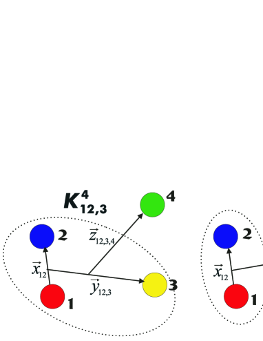
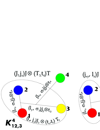
Figure 2: ”(Color online)” Figure [a]: FY components $K$ and $H$. Asymptotically, as $z\rightarrow\infty$, components K describe 3+1 particle channels, whereas components H contain asymptotic states of 2+2 channels. Figure [b] illustrates the j-j coupling schemes used when developing FYC $K$ and $H$ into partial wave basis.

In theoretical treatment of the problem we use the isospin formalism, i.e. we consider protons and neutrons as being degenerate states of the same particle - nucleon. For a system of identical particles, the FYC are not completely independent, being related by several straightforward symmetry relations. All the 18 FYC can be obtained by the action of the permutation operators on two of them, arbitrarily chosen, provided one is of type $K$ and the other of type $H$. We have chosen $K\equiv\Psi_{12,3}^{4}$ and $H\equiv\Psi_{12}^{34}.$ The four-body problem is solved by determining these two components, which satisfy the system of differential equationsMerk_TMP56 :

$$\left(E-H_{0}-V\right)K = V(P^{+}+P^{-})\left[(1+Q)K+H\right]$$

$$\left(E-H_{0}-V\right)H = V_{12}\tilde{P}\left[(1+Q)K+H\right].$$ (1)

$P^{+}$, $P^{-}$, $\tilde{P}$ and $Q$ are the permutation operators:

$$P^{+} = (P^{-})^{-1}=P_{23}P_{12}$$

$$Q = \varepsilon P_{34}$$

$$\tilde{P} = P_{13}P_{24}=P_{24}P_{13}.$$

Employing operators defined above, systems wave function is given by

$$\Psi=\left[1+(1+P^{+}+P^{-})Q\right](1+P^{+}+P^{-})K+(1+P^{+}+P^{-})(1+\tilde{P})H.$$ (2)

Components $K$ and $H$ are functions in configuration space, and depend also on the internal degrees of freedom of the individual particles (spins and isospins). The configuration space is provided by the position of the different particles, which we describe by using reduced relative coordinates. These coordinates differ from Jacobi coordinates usually employed in Classical Mechanics by factors depending on the particle masses. Use of such coordinates has several big advantages: first center of mass motion can be easily separated, then transition between two bases is equivalent to orthogonal transformation in $R^{3(N-1)}$ space; finally, kinetic energy operator in this basis reduces to multidimensional Laplace operator in corresponding subspaces. Two principally different sets of reduced relative coordinates can be defined. One is associated with the components $K\equiv\Psi_{ij,k}^{l}$:

$$\overrightarrow{x_{ij}}$$

   (3)

where $m_{\ell}$ and $\overrightarrow{r}_{\ell}$ are respectively the mass and the position of the $\ell$-th particle. The coordinate set associated with the components $H\equiv\Psi_{ij}^{kl}$, is defined by:

$$\overrightarrow{x_{ij}}$$

   (4)

The functions $K$ and $H$ are expanded in the basis of partial angular momentum, spin and isospin variables, according to:

$$\Phi_{i}(\vec{x}_{i},\vec{y}_{i},\vec{z}_{i})=\sum_{\alpha}\frac{\mathcal{F}_{i}^{\alpha}(x_{i},y_{i},z_{i})}{x_{i}y_{i}z_{i}}Y_{i}^{\alpha}(\hat{x}_{i},\hat{y}_{i},\hat{z}_{i})$$ (5)

Here $Y_{i}^{\alpha}(\hat{x}_{i},\hat{y}_{i},\hat{z}_{i})$ generalize tripolar harmonics containing spin, isospin and angular momentum variables. Functions $\mathcal{F}_{i}^{\alpha}(x_{i},y_{i},z_{i})$ are so called partial amplitudes, being continuous in radial variables $x,y$ and $z.$ The label $\alpha$ represents the set of intermediate quantum numbers defined in coupling scheme, it includes as well the specification for the type of FY’s component ($K$ or $H$). We have used $j-j$ couplings, represented in Fig. 2 [b], and expressed by:

$$\left[\left\{\left(t_{i}t_{j}\right)_{t_{x}}t_{k}\right\}_{T_{3}}t_{l}\right]_{\mathcal{T}}\left\langle\left\{\left[l_{x}\left(s_{i}s_{j}\right)_{\sigma_{x}}\right]_{j_{x}}\left[l_{y}s_{k}\right]_{j_{y}}\right\}_{J_{3}}\left[l_{z}s_{l}\right]_{j_{z}}\right\rangle_{\mathcal{J}^{\pi}}$$ (6)

for components of $K$-type, and

$$\left[\left(t_{i}t_{j}\right)_{t_{x}}\left(t_{k}t_{l}\right)_{t_{y}}\right]_{\mathcal{T}}\left\langle\left\{\left[l_{x}\left(s_{i}s_{j}\right)_{\sigma_{x}}\right]_{j_{x}}\left[l_{y}\left(s_{k}s_{l}\right)_{\sigma_{y}}\right]_{j_{y}}\right\}_{j_{xy}}l_{z}\right\rangle_{\mathcal{J}^{\pi}}$$ (7)

for the $H$-type components. Here $s_{i}$ and $t_{i}$ are the spin and isospin quantum numbers of the individual particles and $\left(\mathcal{J}^{\pi},\mathcal{T}\right)$ are, respectively, the total angular momentum, parity and isospin of the four-body system. Each amplitude $\mathcal{F}_{i}^{\alpha}(x_{i},y_{i},z_{i})$ is thus labelled by the a set of 12 quantum numbers $\alpha$. The symmetry properties of the wave function in respect to exchange of two particles impose additional constraints. One should have $\left(-\right)^{l_{x}+\sigma_{x}+t_{x}}=\varepsilon$ for the amplitudes derived from any type of components ($K$ or $H$), while for $H-$type amplitudes additional constraint $\left(-\right)^{l_{y}+\sigma_{y}+t_{y}}=\varepsilon$ is valid as well. Since we deal with nucleons (i.e. fermions) Pauli factor $\varepsilon$ is equal -1. The total parity $\pi$ is given by $\left(-\right)^{l_{x}+l_{y}+l_{z}}$, independently of the coupling scheme in use.

By projecting each of the Eqs. (1) on its natural configuration space basis one obtains a system of coupled integrodifferential equations. In general one has an infinite number of coupled equations. Note that, contrary to the 3N problem, the number of partial FY amplitudes is infinite even when the pair interaction is restricted to a finite number of partial waves. This divergence comes from the existence of additional degree of freedom $l_{z}$ in the expansion of the $K$-type components. Therefore we are obliged to make additional truncations in numerical calculations by taking into account only the most relevant amplitudes.

II.2 Boundary conditions

Equations (1) are not complete and should be complemented with the appropriate boundary conditions. Boundary conditions can be written in the Dirichlet form. First FY amplitudes, for bound as well as for scattering states, satisfy the regularity conditions:

$$\mathcal{F}_{i}^{\alpha}(0,y_{i},z_{i})=\mathcal{F}_{i}^{\alpha}(x_{i},0,z_{i})=\mathcal{F}_{i}^{\alpha}(x_{i},y_{i},0)=0$$ (8)

For the bound state problem, the wave function is exponentially decreasing and therefore the regularity conditions can be completed by forcing the amplitudes $\mathcal{F}_{i}^{\alpha}$ to vanish at the borders of the hypercube $\left[0,X_{\max}\right]\times\left[0,Y_{\max}\right]\times\left[0,Z_{\max}\right]$, i.e.:

$$\mathcal{F}_{i}^{\alpha}(X_{\max},y_{i},z_{i})=\mathcal{F}_{i}^{\alpha}(x_{i},Y_{\max},z_{i})=\mathcal{F}_{i}^{\alpha}(x_{i},y_{i},Z_{\max})=0$$ (9)

For the elastic scattering problem the boundary conditions are implemented by imposing at large values of $z$ the asymptotic behavior of the solution. In case of N+NNN elastic scattering we impose at $Z_{\max}$ the solution of the 3N problem for all the quantum numbers, corresponding to the open channel $\alpha_{a}$:

$$\mathcal{F}_{i}^{\alpha_{a}}(x_{i},y_{i},Z_{\max})=f_{i}^{\alpha_{a}}(x_{i},y_{i})$$ (10)

Functions $f_{i}^{\alpha_{a}}(x_{i},y_{i})$ are the Faddeev amplitudes obtained after solving corresponding 3N bound state problem. Indeed, below the first inelastic threshold, at large values of $z$, the solution of (1) factorizes into a bound state solution of 3N Faddeev equations and a plane wave propagating in $z$ direction with the momentum $k_{\alpha_{a}}=\sqrt{\frac{m}{\hbar^{2}}\left(E_{cm}-E_{3N}\right)}$. One has:

$$\mathcal{F}_{i}^{\alpha_{a}}(x_{i},y_{i},z_{i})\sim f_{i}^{\alpha_{a}}(x_{i},y_{i})\left[\hat{\jmath}_{l_{z}}(k_{\alpha_{a}}z_{i})+\tan(\delta)\hat{n}_{l_{z}}(k_{\alpha_{a}}z_{i})\right]$$

There are two different ways to obtain the scattering observables. The easier one is to extract the scattering phases from the tail of the solution, namely taking logarithmic derivative of the open channel’s $K$ amplitude $\alpha_{a}$ in the asymptotic region:

$$\tan\delta=\frac{k_{\alpha_{a}}\hat{\jmath}_{l}^{\prime}(k_{\alpha_{a}}z_{i})-\frac{\partial_{z_{i}}\mathcal{F}_{i}^{\alpha_{a}}(x_{i},y_{i},z_{i})}{\mathcal{F}_{i}^{\alpha_{a}}(x_{i},y_{i},z_{i})}\hat{\jmath}_{l}(k_{\alpha_{a}}z_{i})}{\frac{\partial_{z_{i}}\mathcal{F}_{i}^{\alpha_{a}}(x_{i},y_{i},z_{i})}{\mathcal{F}_{i}^{\alpha_{a}}(x_{i},y_{i},z_{i})}\hat{n}_{l}(k_{\alpha_{a}}z_{i})-k_{\alpha_{a}}\hat{n}_{l}^{\prime}(k_{\alpha_{a}}z_{i})}$$ (11)

This result can be independently verified by using integral representation of the phase shifts

$$\sin\delta=-\frac{m}{\hslash^{2}}\int\Phi_{\alpha_{a}}^{(123)}(\vec{x}_{i},\vec{y}_{i})\hat{\jmath}_{l}(k_{\alpha_{a}}z)(V_{14}+V_{24}+V_{34})\Psi(\vec{x}_{i},\vec{y}_{i},\vec{z}_{i})dV.$$ (12)

Here $\Phi_{\alpha_{a}}^{(123)}(\vec{x}_{i},\vec{y}_{i})$ is a 3N bound state wave function composed by particles (1,2,3). This wave function is considered to be normalized to unity. Asymptotes of the wave function $\Psi(\vec{x}_{i},\vec{y}_{i},\vec{z}_{i})$ is considered to have the same normalization as $\Phi_{\alpha_{a}}^{(123)}(\vec{x}_{i},\vec{y}_{i})$, i.e. it tends to:

$$\Psi(\vec{x}_{i},\vec{y}_{i},\vec{z}_{i})=\Phi_{\alpha_{a}}^{(123)}\left(\vec{x}_{i},\vec{y}_{i}\right)\left[\hat{\jmath}_{l_{z}}(k_{\alpha_{a}}z_{i})+\tan(\delta)\hat{n}_{l_{z}}(k_{\alpha_{a}}z_{i})\right].$$ (13)

A detailed discussion on these technical aspects can be found in These_Fred_97 ; These_Rimas_04 .

II.3
Numerical solution

In order to solve the set of integro-differential equations – obtained when projecting eq.(1) in conjunction with the appropriate boundary conditions into partial wave basis – components $\mathcal{F}_{i}^{\alpha}$ are expanded in terms of piecewise Hermite spline basis.

$$\mathcal{F}_{i}^{\alpha}(x,y,z)=\sum c^{\alpha}_{ijkl}S_{j}(x)S_{k}(y)S_{l}(z)$$

In this way, integro-differential equations are converted into an equivalent linear algebra problem with unknown spline expansion coefficients $c^{\alpha}_{ijkl}$ to determine. In case of bound state problem eigenvalue-eigenvector problem is obtained:

$$Ac=EBc,$$ (14)

where $A$ and $B$ are square matrices, while $E$ and $c$ are respectively unknown eigenvalue(s) and its eigenvector(s) to determine. In case of elastic scattering problem, a system of linear algebra equations is obtained:

$$\left[A-E_{cm}B\right]c=b$$ (15)

where $b$ is an inhomogeneous term imposed by the boundary conditions eq.(10). Numerical methods used for solving these large scale $N\sim 10^{7}$ eigenvalue problems and linear systems are given in These_Rimas_04 .

III Results and discussion

We have used in our calculations four different Doleschall potentials derived in references D_NPA602_96 ; D_FBS_98 ; DB_FBS_99 ; DB_PRC62_00 ; DB_NPA684_01 ; DBPP_PRC67_03 ; D_PRC_04 . Hereafter, INOY96 denotes the SB+SDA version of the potential defined in D_NPA602_96 ; D_FBS_98 . It consists in short-range non local potentials in ¹S₀ and ³SD₁ partial waves continued with a local Yukawa tail outside R=4 fm. The other partial waves are taken from AV18. INOY03 denotes the IS version considered in Ref. DBPP_PRC67_03 . It is an updated version of INOY96 which has a smaller non locality range (R=2 fm) and provides a more accurate description of 2N observables. INOY04 and INOY04’ are the two most recent versions D_PRC_04 having the same ¹S₀ and ³SD₁ potentials as INOY03, completed with the newly defined non local potentials in P- and D- waves. As in the preceding models, higher partial waves are also taken from AV18.

All the results have been obtained considering equal masses for neutrons and protons ($m_{n}=m_{p}=m$) with ${\frac{\hbar^{2}}{m}}=41.47$ MeV fm². As mentioned in section II.1 we have used isospin formalism, furthermore assuming the total isospin quantum number $\mathcal{T}$ to be conserved.

III.1 3N system

We will start with the presentation of our results concerning 3N systems. Binding energies for ³H and ³He nuclei are summarized in Table 1. In order to control our accuracy, we have included in this table the results of AV18 AV18_PRC_95 with and without Urbana IX three-nucleon force UIX . One can see that we are in close agreement with the benchmark calculations of Ref. Bench_the . Our results concerning non-local potentials are slightly different from those given in DBPP_PRC67_03 ; D_PRC_04 . The small deviations ($\approx$ 15 keV) come from isospin breaking effects which were fully included in Doleschall calculations DPC while, as discussed in the above section, they were only approximately taken into account in ours. These isospin effects for AV18+UIX have also been evaluated in Bench_the and were found to be of about 5 keV, i.e. three times less than in non-local models. In any case, the small differences related to isospin approximation can not overcast the main achievement of these non local interactions: the ability to reproduce experimental 3N binding energies without three-nucleon force. One can also remark from Table 1 that, while the binding energies obtained with AV18+UIX are in good agreement with the experimental data, the value of $\Delta B=B_{3H}-B_{3He}$ is better reproduced by non local models.

Table 1: ³H and ³He binding energies (in MeV) calculated with various versions of non-local Doleschall potentials and with AV18+UIX model. Results are compared to experimental values and previous calculations. $\Delta B$ denotes the difference between ³H and ³He binding energies

	3H		3He		$\triangle$B
	this work	other	this work	other	this work	other
INOY96	8.556		7.882		0.674
INOY03	8.497	8.482 DBPP_PRC67_03	7.734	7.718 DBPP_PRC67_03	0.763	0.764
INOY04	8.476		7.711		0.765
INOY04’	8.464	8.481 D_PRC_04	7.704	7.718 D_PRC_04	0.760	0.763
AV18	7.616	7.618(2)Bench_the	6.914	6.917(2)Bench_the	0.699
AV18+UIX	8.473	8.474(4)Bench_the	7.739	7.742(4)Bench_the	0.734
Exp.	8.482		7.718		0.764

The analysis of the 3N binding energies is shown in Table 2. One can see that the major contribution to binding is due to the non-local short range interaction terms $<V_{nl}>$. Contributions from the local part – coming either from long range Yukawa tail or from higher partial waves – are marginal in INOY96 model and remain less than 15% in the other ones.

Comparison between INOYs and AV18+UIX results is instructive. Both models provide similar energies and rms radii but they result from values of kinetic and potential energies which differ as much as $\sim$ 50%. The introduction of a non-local interaction reduces the short range repulsion between nucleons and makes the potential well more shallow. Deuteron is already obtained with the same binding energy and size as for AV18 model but its wave function does not have, at short distances, the sharp slope due to hard-core repulsion. On the other hand the weaker ³S${}_{1}-^{3}$D₁ coupling in non-local models generates a smaller contribution of D-state. All these effects reduce the average kinetic energy and favor stronger binding in the 3N system, which is more compact than deuteron. If the average size of 3N system between two models is only slightly different, the average kinetic energy of nucleons is sensibly smaller in case of non-local interactions.

Table 2: Expectation values of kinetic ($<T>$) energies, rms radius ($R=\sqrt{<r^{2}>}$) and proton radius $r_{p}$ corresponding to the binding energies of Table 1. The values of the potential energy have been separated into contributions coming from the non-local $<V_{nl}>$ and local $<V_{l}>$ terms of the potential. For AV18+UIX model, $<V_{nl}>$ denotes the contribution of 3NF to potential energy. For ³He, the expectation values of Coulomb interaction have not been included.

	Model	$<T>$ (MeV)	$-<V_{l}>$ (MeV)	$-<V_{nl}>$ (MeV)	$R$ (fm)	$r_{p}$ (fm)
3H	INOY96	34.24	0.776	42.02	1.656	1.561
	INOY03	33.11	5.551	36.06	1.664	1.566
	INOY04	33.01	5.564	35.92	1.667	1.567
	INOY04’	32.97	5.547	35.89	1.668	1.568
	AV18	46.71	54.32	-	1.770	1.654
	AV18+UIX	51.28	58.69	1.140	1.684	1.584
	Exp.					1.60
3He	INOY96	33.64	0.777	41.42	1.684	1.733
	INOY03	32.33	5.512	35.21	1.701	1.752
	INOY04	32.24	5.510	35.08	1.703	1.755
	INOY04’	32.20	5.525	35.05	1.704	1.756
	AV18	45.68	53.30	-	1.809	1.867
	AV18+UIX	50.22	57.60	1.095	1.716	1.767
	Exp.					1.77

The relative contributions (algebraic values) of the most relevant $V_{NN}$ partial waves to ³H potential energy are given in Table 3. The column labelled ”others” denotes the contribution of all partial waves not listed in the table. One can remark the small role of $P$-waves. It was noticed long time ago that triton binding energy basically depends on ¹S₀ and ³S₁-³D₁ $NN$-interactions. Indeed, in absence of tensor force, the 3N ground state would have L=$0$ and S=$\frac{1}{2}$ as conserved quantum numbers and in this case $P$-waves would not contribute at all. The ³S₁-³D₁ tensor coupling introduces an $L=2$ admixture in the wave function. L=1 state appears only in the second order and contributes less than 0.1 %. NN $P$-waves start acting only in the second order as well, which explains their negligible contribution to 3N binding energy, as shown in Table 3. The reduction of the tensor force is also sizeable: ³D₁-waves contribution are considerably smaller for Doleschall interactions than for AV18.

Table 3: Relative contributions of different $V_{NN}$ partial waves to triton potential energy.

	3S1	1S0	3D1	3P2	3P0	1D2	3P1	1P1	3D2	3D3	Others
INOY96	57.94	29.24	12.78	0.1658	0.1506	0.05664	-0.3810	-0.04528	0.04939	0.01505	0.02518
INOY03	58.30	30.31	11.42	0.1350	0.1892	0.04260	-0.4214	-0.05317	0.06144	0.01634	0.02307
INOY04	58.35	30.33	11.38	0.1409	0.1579	0.04843	-0.4304	-0.05495	0.06303	0.06460	0.0113
INOY04’	58.40	30.36	11.37	0.1478	0.7854	0.05061	-0.4368	-0.05711	0.06527	0.04333	0.0089
AV18	45.00	25.30	28.97	0.4466	0.2272	0.1840	-0.3977	-0.03244	0.07952	0.08769	0.1290

Table 4: Neutron-deuteron (nd) scattering lengths (in fm) calculated using Doleschall potentials.

	${}^{2}a_{nd}$ (fm)	${}^{4}a_{nd}$ (fm)
INOY96	0.448	6.34
INOY03	0.523	6.34
INOY04	0.543	6.34
INOY04’	0.553	6.34
AV18	1.26	6.34
AV18+UIX	0.595	6.34
Exp.	0.65$\pm$0.04	6.35$\pm$0.02

The calculated n-d scattering lengths are presented in Table 4. The quartet value (⁴a), corresponding to $J^{\pi}=\frac{3}{2}^{+}$ state, is independent of the interaction model in use, furthermore being in full agreement with the experimental one. This robustness is due to the strong Pauli repulsion, prohibiting two neutrons to get close to each other. It follows that only ³S${}_{1}-^{3}$D₁ V_np waves are important in describing $J^{\pi}=\frac{3}{2}^{+}$ state and still only through its, well controlled, long range part. Therefore, this state does not contain any off-shell physics and can be successfully described by any potential model, provided it reproduces the $J^{\pi}=1^{+}$ np scattering observables.

The integral representation of the phase shifts, eq. (12), is used to study the role of different V_NN partial waves. In Table 5 are given the relative contributions to this integral. Their sum, in algebraic values, is normalized to 100. Results for n-d doublet scattering length (²a) are presented in the upper half of the table and the quartet ones in the lower part. It can be seen that for $J^{\pi}=\frac{3}{2}^{+}$, NN waves other than ³S₁ contribute by less than 0.1%, which confirms the statements above. The situation is different for ²a which results mainly from a cancellation between ¹S₀ and ³S₁ and is more sensitive to higher NN partial waves, showing a deeper impact into the off-shell physics. Due to the smallness of ²a, all the interaction effects have to be taken into account very accurately. In particular, its value is very sensitive to the electromagnetic (e.m.) interaction terms. The differences between INOY predictions and the experiment can therefore be caused by the absence of e.m. terms in these models. On the contrary e.m. corrections were properly included in AV18+UIX results. In any case the small discrepancy with data has no consequences in phenomenology, since ²a is by one order of magnitude smaller than ⁴a and its relative contribution to the scattering cross sections is negligible.

Table 5: Relative contributions of different NN interaction waves in n-d integral scattering lengths. Doublet value is in the upper half of the table and quartet in the lower

	3S1	1S0	3D1	3P2	3P0	1D2	3P1	1P1	3D2	3D3	Other.
INOY96	-685.3	800.3	-20.14	2.664	-1.240	-5.097	-11.97	20.07	-0.7484	0.6967	0.7998
INOY03	-572.6	685.2	-16.73	1.955	0.2399	-4.523	-10.95	16.73	-0.6048	0.3972	0.8616
INOY04	-549.6	662.4	-16.28	1.997	-0.3862	-4.257	-10.31	15.66	-0.5025	0.3749	0.8932
INOY04’	-538.5	650.8	-15.92	2.127	-1.076	-4.167	-9.308	15.25	-0.4694	0.3563	0.8825
AV18	-195.5	293.5	-4.283	4.779	0.6261	-0.3768	-5.944	6.190	-0.3316	0.9574	0.3281
INOY96	100.1	-0.0297	0.0183	-0.2708	-0.5036	-0.1510	0.8177	0.0190	-0.1644	0.0076	0.0312
INOY03	100.0	-0.0288	0.0199	-0.2694	-0.4640	-0.1529	0.8180	0.0192	-0.1641	0.00742	0.0315
INOY04	100.1	-0.0283	0.0197	-0.2707	-0.4938	-0.1515	0.8343	0.0189	-0.1653	-0.0006	0.0480
INOY04’	99.98	-0.0279	0.0195	-0.2675	-0.4973	-0.1503	0.9043	0.0188	-0.1651	-0.0004	0.0479
AV18	100.1	-0.0400	0.0097	-0.2672	-0.4870	-0.2577	0.8081	0.0252	-0.1691	0.0096	0.0361

III.2 4N system

Our results concerning the $\alpha$-particle binding energy are displayed in Table 6. Two series of calculations were performed, including (upper half of the table) and neglecting (lower half) Coulomb repulsion between protons. This latter interaction was provided by Argonne group in their AV18 code AV18_PRC_95 and takes into account proton finite size effects.

Table 6: Binding energy B (in MeV) and rms radius R (in fm) for ⁴He ground state obtained with Doleschall and AV18+UIX potentials. The lower part contains Coulomb force. Energies presented in the two last lines of the table respectively for AV18 and AV18+UIX models have been taken from reference Nogga_alp ; Nogga_thesis , whereas rms radius from reference PPWC_PRC64_01 .

Pot.	$<T>$	$-<V>$	$B$	$R$
INOY96	72.80	103.8	31.00	1.353
INOY03	69.89	99.94	30.04	1.369
INOY04	69.49	99.41	29.91	1.372
INOY04’	69.46	99.36	29.88	1.372
AV18	98.69	123.6	24.95	1.511
Pot.	$<T>$	$-<V>$	$-<E>$	$R$
INOY96	72.45	102.7	30.19	1.358
INOY03	69.54	98.79	29.24	1.373
INOY04	69.14	98.62	29.11	1.377
INOY04’	69.11	98.19	29.09	1.376
AV18	97.77	122.1	24.22	1.516
	97.80	122.0	24.23   Nogga_alp ; Nogga_thesis
AV18+UIX	113.2	141.7	28.50   Nogga_alp ; Nogga_thesis	1.44 PPWC_PRC64_01
Exp			28.30	1.47

Calculations have been done by considering isospin averaged pair interaction, i.e.:

$$V_{t_{1}t_{2}}=P_{nn}(t_{1},t_{2})V_{nn}+P_{pp}(t_{1},t_{2})V_{pp}+P_{np}(t_{1},t_{2})V_{np}$$

where $(t_{1},t_{2})$ are the isospin quantum numbers of FY amplitudes in equation (5). They respectively represent $(t_{x},T_{3})$ for $K$-type amplitudes and $(t_{x},t_{y})$ for $H$-type. $P_{nn},P_{pp}$ and $P_{np}$ are the probabilities of finding respectively nn, pp and np pairs in a given isospin state. Note that, since the number of protons and neutrons in $\alpha$-particle is equal, one has $P_{nn}(t_{1},t_{2})=P_{pp}(t_{1},t_{2})$.

As in 3N calculations, we have neglected isospin breaking effects, considering $\alpha$-particle as a pure $\mathcal{T}=0$ state. Contributions of $\mathcal{T}=1,2$ admixture were calculated for AV18 and AV18+UIX models in Nogga_alp and found to be as small as 10 keV. Results for 3N system presented in last section showed that Doleschall non-local models are more sensible to isospin breaking: they account for $\approx$15 keV in ³H compared to $\approx$5 keV in AV18+UIX Bench_the . In any case, for the alpha particle these effects should not exceed some 50 keV and will not affect the physics discussed below. Notice also that Coulomb corrections obtained by non-local models exceed by 70 keV those obtained by AV18, due to the different rms radii they give.

As mentioned in section (II.1), FY calculations have been performed in the $j-j$ coupling scheme. The following truncations in the partial wave expansion of amplitudes were used: (i) V_NN waves limited to $l_{x}\leq 3$ but always including tensor-coupled partners, i.e. involving the set ${}^{1}S_{0},^{3}SD_{1}$, ${}^{1}P_{1},^{3}P_{0},^{3}PF_{2},^{3}P_{1}$, ${}^{1}D_{2},^{3}DG_{3},^{3}D_{2}$, ${}^{1}F_{3},^{3}FH_{4},^{3}F_{3}$ and (ii) $l_{x}+l_{y}+l_{z}\leq 10$.

Convergence was studied as a function of $j_{yz}$=max($j_{y}$,$j_{z}$) for K-like components and $j_{yz}$=max($j_{y}$,$l_{z})$ for H-like, starting with $j_{yz}\leq 1$. In Table 7 we present the $\alpha$-particle binding energy results for INOY04’ and AV18 models respectively. The convergence is rather smooth, except when passing from $j_{yz}\leq 5$ to $j_{yz}\leq 6$. We think this is an artefact of our truncation procedure which keeps fixed the basis set in the x-coordinate. Note that the agreement between our results for AV18 potential and those, given in reference Nogga_alp ; Nogga_thesis , is very good. From results displayed on Table 7, as well as from analogous convergence patterns seen in 3N calculations, we conclude that Doleschall potentials converge more rapidly than AV18. This is probably due to their weaker tensor force, resulting into wave functions with stronger spherical symmetry.

Table 7: Results of $\alpha$-particle binding energy (in MeV) for INOY04’ and AV18 models with V_NN interaction limited to $l_{x}\leq 3$ (see text) and partial wave basis limited to $l_{x}+l_{y}+l_{z}\leq 10$. The convergence was searched as a function of $j_{yz}$=max($j_{y}$,$j_{z}$) for K-like components and $j_{yz}$=max($j_{y}$,$j_{z})$ for H-like. Last line, denoted by *, contains additional calculations with NN interaction waves up to $j_{x}\leq 6$ and $l_{x}+l_{y}+l_{z}\leq 12$.

$j_{yz}$	INOY04’	AV18
1	28.094
2	28.661
3	28.967
4	28.971	23.897
5	28.974	23.920
6	29.084	24.233
7	29.085	24.226
	29.085	24.223

To our opinion the main conclusion of the results displayed in Table 6 is the possibility offered by the INOY models to provide a satisfactory description of A=4 nuclei in terms of two-body forces alone, as it is already the case for A=2 and 3. One can argue that this agreement is not yet fully realized in their present version, for they all slightly overbind the experimental value: the most favorable version (INOY04’) still exceeds by 0.79 MeV the ⁴He binding energy. One should however remark that this result is obtained without adjusting any additional parameter with respect to A=3. On the other hand, the difference between INOY96 and INOY04’ – due essentially to different parameterizations of their non local short range parts – is 1.1 MeV. It seems thus possible, by a finer tuning, to reach an even more precise description of A=4 in a next generation of potentials. If they are not contradicted by other aspects of the phenomenology, INOY models offer an alternative description permitting to avoid three-nucleon forces.

Results of Table 6 have been gathered in a Tjon plot – see Figure 3 – which displays the correlation between ³H and ⁴He binding energies for various NN potentials. One can see that, due to the small overbinding of $\alpha$-particle, INOY results (diamond symbols) are outside the line formed by realistic local model predictions and, except for INOY96, are almost superimposed to CD Bonn + TM value.

INOY03, INOY04 and INOY04’ models, which differ in their P-wave structure, give very close results while INOY96, which has a different non-local S-wave structure, falls out further apart. This indicates that the S-waves are the key point in binding $\alpha$-particle and in order to improve the agreement with the experimental value a better tuning in the ³S₁-³D₁ and ¹S₀ could be helpful.

Proton rms radii predicted by INOY potentials deserve some comments. One can see already in 3N systems (see Tab. 2) that they are slightly smaller than the experimental ones. For $\alpha$-particle we have only calculated average rms of nucleons, without making distinction between neutrons and protons. The real value of protons rms should be slightly larger. However, since Coulomb interaction has very small effect on the alpha particle wave function (rms radii calculated by taking Coulomb interaction into and without account differ only in fourth digit) this value can not differ by more than 0.5%. One can therefore see that protons rms provided by INOY model are already by 6% smaller than the experimental one, compared to 1-2% in 3N complex. This fact clearly demonstrates that INOY interactions are too soft, resulting into a faster condensation of the nuclear matter. In order to improve the agreement one should try to increase the short range repulsion between the nucleons. This would inevitably imply a reduction of 3N binding energies, although this reduction is not necessarily very large. If one chooses the ITF ³S₁-³D₁ and ISA ¹S₀ potential versions from DB_NPA684_01 , which give the smallest probabilities to find nucleons close to each other in 2N systems, the resulting triton underbinding will be of only $\sim$50 keV.

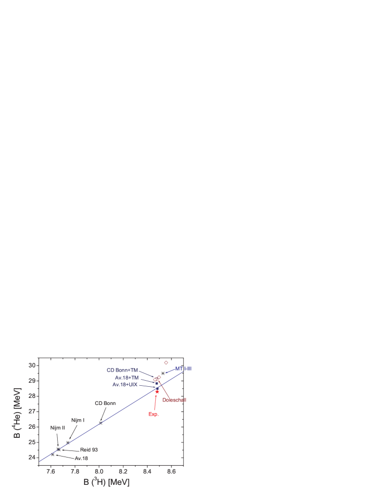
Figure 3: ”(Color online)” Tjon-line for the local and non local NN potentials.

Let us finally consider the n+³H elastic scattering. This is, in principle, the simplest 4N reaction, being almost a pure $\mathcal{T}=1$ isospin state and free of Coulomb interaction. However, its simplicity is only apparent. In fact, n+³H is a system with very large neutron excess ($\eta={N-Z\over A}=0.5$). The only stable nucleus having a neutron excess equally large is ⁸He. Let us remind that AV18+UIX hamiltonian, faces increasing difficulty when describing neutron rich nuclei. The more elaborate 3NF model, namely Illinois PPWC_PRC64_01 , even though being able to improve the agreement with experimental data, still suffers from similar discrepancies These_Rimas_04 . In addition, the n+³H system contains several nearthreshold resonances of negative parity (see Fig 4), which strongly affect the scattering observables near $E_{cm}\approx 3$ MeV. Their internal dynamics is richer than for bound states and it is not clear that they can be described by using the same recipes than the one used for solving the underbinding problem. The description of the n+³H cross sections in the resonance region is therefore a very challenging task for nucleon-nucleon interaction models.

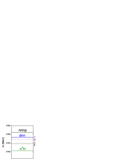
Figure 4: ”(Color online)” Negative parity resonance above the n+t threshold

Table 8: n+³H singlet (J^π=0⁺), triplet (J^π=1⁺) and coherent scattering lengths (in fm) along with zero energy cross sections. Different model results are compared with the experimental data.

Pot.	a${}_{0^{+}}$ (fm)	a${}_{1^{+}}$ (fm)	ac (fm)	$\sigma$ (fm2)
INOY04	4.00	3.52	3.64	166.5
INOY04’	4.00	3.52	3.64	166.8
AV18	4.27	3.71	3.85	187.0
AV18+UIX	4.04	3.60	3.71	173.4
Experimental	3.70$\pm$0.62	3.70$\pm$0.21	3.82$\pm$0.07 HRCK_ZPA_81	170$\pm$3PBS_PRC_80
	4.98$\pm$0.29	3.13$\pm$0.11	3.59$\pm$0.02 RTWW_PLB_85
	2.10$\pm$0.31	4.05$\pm$0.09
	4.45$\pm$0.10	3.32$\pm$0.02	3.607$\pm$0.017 HDSBP_PRC_90

We have performed extensive calculations of the n+³H scattering states only by using the INOY04 potential. The model dependency of the results was checked at $E_{cm}$=0 and 3 MeV with INOY04’. We present in Table 8 the calculated singlet ($a_{0^{+}}$) and triplet ($a_{1^{+}}$) scattering lengths together with the deduced coherent value

$$a_{c}=\frac{1}{4}\left(a_{0^{+}}+3a_{1^{+}}\right)$$ (16)

and the zero energy cross section

$$\sigma(0)=\pi\left(a_{0^{+}}^{2}+3a_{1^{+}}^{2}\right)$$ (17)

Results for AV18 and AV18+UIX models have also been obtained and agree at 1% level with those given in Ref. VRK_98 .

The $J^{\pi}=0^{+}$ and $1^{+}$ positive parity states, determining the low energy behavior of the n+³H cross section, do not have any $S$-matrix singularity, except the triton bound state threshold. It is therefore not surprising that the n+³H scattering lengths are found to be correlated with 3N binding energy, in a similar way as $n+d$ doublet scattering length is Philips . This is the reason why realistic local interaction models, providing too low 3N binding energies, overestimate n+³H zero energy cross sections. Once triton binding energy is corrected, for instance by implementing 3NF, a value close to the experimental one is automatically obtained. From Table 8 it can be seen that Doleschall potential agrees with the lower bound of experimentally measured zero energy cross section, whereas AV18+UIX model coincides with its upper bound. The zero energy scattering cross section is thus fairly well reproduced.

Figure 5: ”(Color online)” Extraction procedure for n+³H singlet ($a_{0^{+}}$) and triplet ($a_{1^{+}}$) scattering lengths from measurements of zero energy cross section (elliptic band) PBS_PRC_80 and coherent scattering length (linear bands) HRCK_ZPA_81 ; RTWW_PLB_85 ; HDSBP_PRC_90 . The values of $a_{i}$ are given by the intersection of these two curves. Band widths are related to experimental errors and, even being small, they make their determination very unstable.

The situation with scattering lengths looks more precarious. The values found in literature are hardly compatible with each other C_NPA684_01 as it can be seen in Table 8. The usual way to get $a_{i}$ is to express them in terms of the measured quantities $a_{c}$ and $\sigma(0)$, by reversing relations (16) and (17). This procedure, represented in Fig. 5, is numerically unstable. Indeed, once $\sigma(0)$ is fixed, the domain of permitted $a_{1^{+}}$ and $a_{0^{+}}$ values is given by the ellipse of eq. (17) in the $(a_{0^{+}},a_{1^{+}})$ plane. Since there are uncertainties in $\sigma(0)$, the permitted values of scattering lengths are trapped in-between two ellipsis (dot curves in Fig. 5). On the other hand, each measurement of $a_{c}$ restricts $a_{1^{+}}$ and $a_{0^{+}}$ values to lie on a straight line which spreads into a band due to experimental errors (see Figure). The lower band displayed in Figure 5 follows from the R-matrix analysis result $a_{c}=3.607\pm 0.017$ $fm$ HDSBP_PRC_90 , while the upper one comes from the experimental measurement $a_{c}=3.82\pm 0.07$ fm from HRCK_ZPA_81 . By assuming an exact value of $a_{c}$, e.g. $a_{c}=3.624$ $fm$ given by the top of the lower band, the present – though small – experimental error in $\sigma(0)$ leads to two sets of solutions which spread over a wide range: (i) $a_{0^{+}}=[4.31-5.00]$, $a_{1^{+}}=[3.16-3.40]$ and (ii) $a_{0^{+}}=[2.25-2.94]$, $a_{1^{+}}=[3.85-4.08]$ fm. This example illustrates the difficulty of extracting reliable values of $a_{0^{+}}$ and $a_{1^{+}}$. The accurate determination of $a_{i}$ would require to gain one order of magnitude in measuring both $\sigma(0)$ and $a_{c}$.

As it can be seen also from Figure 5, the coherent scattering length value $a_{c}=3.82\pm 0.07$ fm of reference HRCK_ZPA_81 is in evident disagreement with the experimentally measured zero energy cross sections, since it does not intersect $\sigma(0)$ ellipsis. In this respect, the more recent values $a_{c}=3.607\pm 0.017$ fm HDSBP_PRC_90 and $a_{c}=3.59\pm 0.02$ fm RTWW_PLB_85 are more reliable. Doleschall non-local potential provides $a_{c}=3.63$ fm, one standard deviation from these measurements, and seems to be more compatible with data than AV18+UIX model. Fig. 5 suggests also that the real value of the zero energy cross section should coincide with the lower bound of the experimental result.

The success in describing n+³H scattering lengths by Doleschall potential is visible at slightly higher energies as well. In Figure 6 we present our calculated elastic cross section for the scattering energies in the n+³H center of mass energy range from 0 to 3 MeV. Doleschall potential reproduces experimental cross sections near its minima at E${}_{cm}\approx 0.4$ MeV. In this region both MT I-III – the only potential known to us being capable to reproduce the resonant region CC_PRC58_98 – and AV18+UIX overestimate the experimental value.

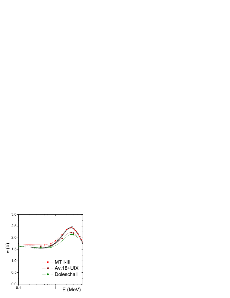
Figure 6: ”(Color online)” Comparison between experimental and theoretical n-³H total cross section calculated with several local and non-local NN potentials.

In previous works These_Fred_97 ; CCG_NPA631_98 ; CCG_PLB447_99 ; C_FBS12_00 ; C_NPA684_01 we pointed out that local realistic interaction models underestimate the cross sections near the resonance peak, $E_{cm}=$3 MeV. At that time, calculations had been however performed with a limited number of partial waves and the failure was attributed in Ref. F_PRL83_99 to a lack of convergence. Recently we have considerably increased our basis set and have shown that the disagreement is indeed a consequence of nuclear models These_Rimas_04 ; LC_TUNL . The convergence of our present results is shown in Table 9, following the same truncation criteria as for $\alpha$-particle (see Table 7). The number of FY partial amplitudes involved in n+t scattering calculations is considerably larger than for a pure $0^{+}$ bound state and we have not been able to go in the PWB as far than in Table 7. One can however remark that results displayed on Table 9 converge pretty well, and provide at least three digit accuracy.

Table 9: Convergence of n+t scattering lengths and selected phaseshifts at E_cm=2.625 MeV for INOY04 model. Corresponding mixing parameters are given in parentheses.

$j_{yz}$	$a_{0}^{+}$ (fm)	$a_{1}^{+}$ (fm)	$\delta(1^{+})$ (deg)	$\delta(1^{-})$ (deg)
1	3.889	3.609	—	—
2	3.995	3.508	-56.13 -0.757 (0.803)	21.32 39.54 (-42.05)
3	3.995	3.513	-56.12 -0.759 (0.803)	21.39 39.74 (-43.06)
4	3.995	3.515	-56.12 -0.759 (0.803)	21.39 39.76 (-43.16)

Implementation of 3NF is just able to improve zero-energy cross sections and is not efficient at the resonance energies. Doleschall non-local potentials seem to suffer from a similar defect: the phase shifts obtained using INOY04 are even slightly smaller in their absolute value (except for 2^- state) than those obtained with local potentials and the total cross section is slightly worse. In fact the reduction of positive-parity phase shifts is a consequence of improving triton binding energies. As was previously discussed, n+³H scattering lengths are linearly correlated with the triton binding energy. Whatever the way one uses to increase triton binding, by means of non-local interaction or 3NF, the final result will inevitably be a reduction of 0⁺ and 1⁺ n+³H scattering lengths and low energy phase shifts (in absolute value). It turns out that by the same way, we reduce in absolute value the 0^- and 1^- phase shifts. Only 2^- phases are slightly increased in both AV18+UIX and Doleschall models. Thus we have a real puzzle for the interaction models: on one hand they have to reduce low energy cross sections, while on the other hand cross sections in the resonance region should be significantly increased. The fact that all realistic interactions systematically suffer in the resonance region let us believe that the underlying reason of this disagreement is not related to the non-locality or to 3NF effects. The observed discrepancies have different background than the underbinding problem. Where does this failure comes from?

When analyzing n+³H cross sections in the resonance region, one should first recall their origin. They are negative parity states and their symmetry is consequently different from the positive parity ones, which are dominated by S-waves. The good agreement of the scattering lengths provided by Doleschall potential as well as its success in reproducing the low energy cross section minima, makes us believe that the positive parity phases are quite well reproduced in the resonance region as well. On the other hand, negative parity phase shifts should be rather far from reality, causing a disagreement with the experimental data.

Table 10: Relative contributions of different NN interaction waves in n-³H integral scattering lengths (second half of the table).

	$J^{\pi}$	$E_{cm}$ (MeV)	1S0	3S1	1P1	3P0	3P1	3P2	1D2	3D1	3D2	3D3	others
INOY04’	0+	0.0	75.95	22.83	3.588	-1.301	1.942	-0.8112	-0.8661	-1.433	0.1145	0.006131	0.0188
INOY04’	0+	3.0	79.79	19.68	3.413	-1.046	1.913	-0.5796	-0.5796	-1.837	0.0745	0.005113	-0.0803
INOY04	0-	3.0	61.93	67.82	-0.3569	32.97	-26.58	2.190	1.897	-40.41	0.6489	-0.6528	0.5551
INOY04’	0-	3.0	64.16	70.14	-0.3769	32.83	-29.71	2.305	1.987	-41.90	0.6723	-0.6919	0.5750
INOY04’	2-	3.0	39.75	54.90	-0.1640	1.063	-6.893	14.29	0.0970	-3.182	0.1476	.0001	0.0092

To understand the possible source of such a disagreement, we have calculated – as for nd case – the relative contribution of the different NN partial waves in the integral expression of the phase shifts (12). The obtained results are summarized in Table 10. First two rows correspond to the 0⁺ at E=0 and E=3 MeV. One can see that positive parity states are completely controlled by the interaction in ³SD₁ and ¹S₀ waves, at zero energies as well as at E_cm=3 MeV, close to resonance peak. The role of higher partial waves is marginal. The situation changes dramatically in negative parity states (values on 3-5 rows). Contribution of P-wave interactions becomes comparable to S-wave. On the other hand, the non triviality of physics in the resonance region is reflected by the strong compensation of different P-waves as well as ${}^{3}D_{1}$ and ${}^{3}S_{1}$ components in ³SD₁ channel. In addition, different P-waves dominate in different states: in 2^- state, the ³P₂ waves are the most relevant, whereas ³P₀ is almost negligible; in 0^- state, the ${}^{3}P_{0}$ wave has the largest contribution, while $3P_{2}$ fades away.

Finally, we would like to comment that all the observables where NN P-waves are contributing, have tendency to disagree with the experimental data. A small disagreement can already be seen in n-d doublet scattering lengths (Table 4), whereas triton, described by the same quantum numbers but where P-waves are negligible, is perfectly reproduced. Other examples could be the 3N analyzing powers P_waves_Gloe ; P_waves_Pisa , as well as increasing discrepancy when describing binding energies of neutron rich nuclei (see Figure 1). One should also recall that P-waves in most of the NN interactions are tuned on n-p and p-p data. Moreover, p-p P-waves are overcasted by Coulomb repulsion, while n-n P-waves are not directly controlled by experiment at all. This study suggests that CSB and CIB effects can be sizeable in n-n P-waves and provide a possible explanation for the disagreement observed in n-³H resonance region.

IV Conclusions

During the last decade, a series of non-local NN potentials has been developed by Doleschall and collaborators and were found to provide an overall satisfactory description of the 2N and 3N system. If they left unsolved some of the theoretical nuclear problems – like the so called $A_{y}$ puzzle – they constitute an undoubted success for their ability to reproduce the experimental binding energy of ³H and ³He nuclei without adding three-nucleon forces.

In this work, we have examined the possibilities for these non-local potentials to describe the 4N system as well. This system is a cornerstone in the nuclear ab-initio calculations and a crucial test for the nuclear models. Not only because therein the underbinding problem manifests in its full strength, but also because of the rich variety of scattering states it possesses.

We have found that non-local NN models, could well provide 3N and 4N binding energies in agreement with the experimental data without making explicit use of three-nucleon forces. They offer an alternative solution to cope with the nuclear underbinding problem, than the one offered by the local plus 3NF philosophy.

In their present form, they overbind ⁴He by some 0.7 MeV, a discrepancy much smaller that all the existing models and which reverses the lack of binding observed in most realistic potentials. The fluctuations in the predictions between different versions of the non-local models suggest that a finer parametrization of their internal non-local part could be enough to make them fully successful in that point. The current version seems to be too soft in the short range region, thus giving slightly too small rms radii of light nuclei.

By calculating n+³H scattering states, we have found that Doleschall models are also very encouraging in describing the low energy parameters, providing an even better description than Nijm II or AV18+UIX. However they fail also in reproducing the elastic cross section few MeV above, in the resonance region. In a series of preceding works CCG_NPA631_98 ; CCG_PLB447_99 ; LC_TUNL ; These_Rimas_04 we have shown that local realistic interactions, even implemented with 3NF, underestimate the cross sections at the resonance peak E_cm= 3 MeV. Unfortunately, the non local models do not solve this problem. On the contrary, they even provide slightly smaller values of the cross section. We believe than the reason of this failure is common to all realistic models and lies in the nucleon-nucleon P-waves themselves. The analysis of their contribution shows that, contrary to ⁴He binding energy, they play a crucial role in the n+³H cross sections. If the n-p P-waves seem to be well controlled by the experimental data, one still has a relative freedom in the n-n ones to improve the description.

Acknowledgements: Numerical calculations were performed at Institut du Développement et des Ressources en Informatique Scientifique (IDRIS) from CNRS and at Centre de Calcul Recherche et Technologie (CCRT) from CEA Bruyères le Châtel. We are grateful to the staff members of these two organizations for their kind hospitality and useful advices.

References

- [1] S.R. Beane, P.F.Bedaque, A. Parreno, M.J. Savage, Phys. Lett. B 585 (2004) 106-114
- [2] S. R. Beane, Plenary talk at 17th International IUPAP Conference on Few-body Problems in Physics, June 5-10, 2003, Durham, North Carolina, USA, nucl-th/0308084
- [3] Nuclear Physics with Lattice QCD, White Paper Writing Group, http://www-ctp.mit.edu/ negele/WhitePaper.pdf
- [4] R.B. Wiringa, V.G.J. Stoks, R. Schiavilla, Phys Rev C 51 (1995) 38
- [5] V.G.J. Stoks, R.A.M. Klomp, C.P.F. Terheggen, J.J. de Swart, Phys. Rev. C 49 (1994) 2950
- [6] S.C. Pieper, V.R. Pandharipande, R.B. Wiringa, J. Carlson, Phys. Rev. C 64 (2001) 014001-1
- [7] K. Varga,S.C. Pieper, Y. Suzuki, R.B. Wiringa, Phys. Rev. C 66 (2002) 044310
- [8] A. Nogga, H. Kamada, W. Glöckle and B.R. Barrett, Phys. Rev. C 65 (2002) 054003
- [9] J.L. Friar, G.L. Payne, V.G.J. Stoks, J.J. de Swart, Phys. Lett. B 311 (1993) 4-8
- [10] R. Machleidt, Phys. Rev. C 63 (2001) 024001
- [11] D.R. Entem, R. Machleidt, Phys. Lett. B 524 (2002) 93
- [12] E.Epelbaum, W. Glöckle, U.G. Meissner, Nucl. Phys. A 637 (1998) 107
- [13] E. Epelbaum, W. Glöckle, U.G. Meissner, Nucl. Phys. A671 (2000) 295
- [14] W. Glöckle, W. Polyzou, Few-Body Systems 89 (1990) 97
- [15] W.N. Polyzou, Phys. Rev.C 58 (1998) 91
- [16] A. Stadler, F. Gross, Phys. Rev. Lett. 78 (1997) 26
- [17] P. Doleschall, Nucl. Phys. A 602 (1996) 60
- [18] P. Doleschall, Few-Body Systems 23, (1998) 149
- [19] P. Doleschall and I. Borbély, Few-Body Systems 27, (1999) 1
- [20] P. Doleschall and I. Borbély, Phys. Rev. C62 (2000) 054004
- [21] P. Doleschall and I. Borbély, Nucl. Phys. A 684 (2001)557c
- [22] P. Doleschall, I. Borbély, Z. Papp, W. Plessas, Phys. Rev. C 67 (2003) 064005
- [23] P. Doleschall, to appear in Phys. Rev. C
- [24] A. Amghar, B. Desplanques, Nucl. Phys. A 714 (2003) 502
- [25] V.I. Kukulin, V.N. Pomerantsev, A.Faessler, A.J. Buchmann and E.M. Tursunov, Phys. Rev. C 57 (1998) 535
- [26] R. Lazauskas, PhD Thesis, Université Joseph Fourier, Grenoble (2003); http://tel.ccsd.cnrs.fr/documents/archives0/00/00/41/78/
- [27] L.D. Faddeev, Zh. Eksp. Teor. Fiz. 39, (1960) (Wiley & Sons Inc., 1972). 1459 [Sov. Phys. JETP 12, (1961) 1014
- [28] O.A. Yakubowsky, Sov. J. Nucl. Phys. 5 (1967) 937
- [29] S.P. Merkuriev and S.L. Yakovlev, 56 (1984) 673
- [30] F. Ciesielski, PhD thesis, Université Joseph Fourier, Grenoble (1997)
- [31] B.S. Pudliner, V.R. Pandharipande, J. Carlson and R.B. Wiringa, Phys. Rev. Lett. 74 (1995) 4396
- [32] A. Nogga, A. Kievsky, H. Kamada, W. Glöckle, L.E. Marcucci, S. Rosati and M. Viviani, Phys. Rev. C67 (2003) 034004
- [33] P. Doleschall private communications.
- [34] A. Nogga, Ph.D. thesis, Ruhr-Universität, Bochum 2001
- [35] M. Viviani, S. Rosati, A. Kievsky, Phys. Rev. Lett. 81 (1998) 1580
- [36] A.C. Philips, Phys. Lett. 28 B (1969) 378; Rep. Prog. Phys. 40 (1977) 905
- [37] J. Carbonell, Nucl Phys A 684 (2001) 218
- [38] T.W. Phillips, B.L. Berman, J.D. Seagrave, Phys. Rev. C22 (1980) 384
- [39] S. Hammerschmied, H. Rauch, H. Clerc, U. Kischko, Z. Phys. A302 (1981) 323
- [40] H. Rauch, D. Tuppinger, H. Wolwitsch, T. Wroblewski, Phys. Lett. 165B (1985) 39
- [41] G.M. Hale et al., Phys. Rev. C 42 (1990) 438
- [42] F. Ciesielski, J. Carbonell, C. Gignoux, Nucl. Phys. A631 (1998) 653c
- [43] F. Ciesielski, J. Carbonell, Phys. Rev. C58 (1998) 58 [We notice a misprint in Tab. VIII: and for a given S-line must be inverted, in agreement with Tab. VII]
- [44] F.Ciesielski, J. Carbonell, C. Gignoux, Phys. Lett. B 447 (1999) 199
- [45] J. Carbonell, Few-Body Syst. Suppl. 12 (2000) 439
- [46] R. Lazauskas, J. Carbonell, Contribution to 17th International IUPAP Conference on Few-body Problems in Physics, June 5-10, 2003, Durham, North Carolina; to appear in Nucl. Phys. (2004)
- [47] A.C. Fonseca, Phys. Rev. Lett. 83 (1999) 4021
- [48] M. Viviani, Few-Body Systems Suppl. 10 (1999) 363
- [49] H. Witała, W. Glöckle, Nucl. Phys. A 528 (1991) 48
- [50] W. Tornow, H. Witała and A. Kievsky, Phys. Rev. C 57 (1998) 555