RPA Vector Meson Leptonic Widths

Recent $J=0$ (para) baryonium interpretations of the BES narrow resonance data near the $e^{-}e^{+}\rightarrow p\bar{p}$ threshold suggests the existance of ortho baryonium. To assist future searches we study $J=1$ states, especially vector meson leptonic decays, and report RPA calculations for both light and heavy mesons using a Coulomb-gauge QCD-inspired model. Since the $\phi(1880)$ is the only missing model state, other discovered $J=1$ particles in this region are ortho baryonium candidates.

1 Introduction

Since the November Revolution entailing the discovery of charmonium and universal acceptance of quarks, electron-positron collisions have been an effective method for novel hadronic production. The narrow widths of the $J/\psi$ and subsequently observed $\Upsilon$ led to their interpretation in terms of new quark flavors (see for example appelquist ). These mesons were quarkonium states which predominantly decayed via the electroweak interaction. In a potential quark model their leptonic widths were first calculated schnitzer using

$$\Gamma_{ee}\equiv\Gamma_{V\to e^{-}\ e^{+}}=16\pi\alpha_{\rm EM}^{2}\frac{q^{2}}{M_{V}^{2}}\arrowvert\psi(0)\arrowvert^{2}$$ (1)

with $q$ the charge of the quark in electron units, $M_{V}$ the resonance mass and $\psi(0)$ the wavefunction at the origin. The quantity $\arrowvert\psi(0)\arrowvert^{2}$ also appears in the matrix element of the hyperfine interaction appelquist and therefore its model value for the hyperfine splitting, $\Delta M_{hyp}$, in meson spectra (pseudoscalar-vector meson mass differences) should be simultaneously tested. This also provides a relation between the leptonic width and the hyperfine splitting

$$\Delta M_{hyp}=\frac{1}{6}\left(\frac{9}{\alpha_{EM}^{2}}\frac{\Gamma_{ee}}{M_{V}}\right)^{4/3}M_{V}\ .$$ (2)

However, using this result and the known $\pi$-$\rho$ mass difference, the first prediction appelquist for the charmonium hyperfine splitting failed dramatically. Subsequently, quark models, such as Ref. isgur , incorporating a complex, flavor dependent hyperfine interaction were able to reproduce the hyperfine splittings in various circumstances but fine-tuning was still required since these approaches did not include chiral symmetry. The key point is that the pion is the Goldstone boson of spontaneously broken chiral symmetry which is responsible for its light mass. Indeed more recent and improved chiral approaches lc ; weall find that about 70 % of the $\pi$-$\rho$ splitting is due to chiral symmetry. Consequently, attributing this large 600 MeV splitting entirely to the hyperfine interaction can lead to an inconsistent description of other, less dramatic spectra splittings in baryons, heavy mesons and light meson excited states.

A more fundamental treatment is provided by field-theoretical quark models that dynamically incorporate chiral symmetry. The Nambu and Jona-Lasinio model is one example but the signature contact interaction precludes describing radial excitations (as well as confinement). A similar problem plagues contemporary covariant formulations of the Schwinger-Dyson and Bethe-Salpeter equations that generate unphysical states corresponding to relative time excitations. A more promising approach, which we have utilized weall , is to diagonalize an effective QCD Hamiltonian in the Coulomb-gauge using the chiral symmetry preserving Random Phase Approximation [RPA].

In this paper we apply the RPA to predict vector meson leptonic widths. In addition to further testing our model by confrontation with data we also discuss exotic baryonium states. In view of the recent resonance discovered at BES bes with a nucleon-antinucleon bound state interpretation gao ; kerbikov , we comment on possible vector states in the $1800\ MeV$ region, focusing on the quark model’s, as yet undiscovered, $\phi(1880)$ that naturally fits in our approach.

2 Vector Meson Self-Energy and Width

The width, $\Gamma$, of a hadron is inversely related to its lifetime and can be obtained from its self-energy, $\Sigma(p^{2})$, by $Im\ \Sigma(M^{2})=\Gamma/2$ for a particle with mass $M$ and momentum $p$. For a vector meson the appropriate self-energy contribution at the one $e^{-}e^{+}$ loop level can be computed from the diagram in Fig. 1. This yields

$${\Sigma}=i\frac{g(M^{2})^{2}}{M^{2}}\Pi(M^{2})$$ (3)

where $g(p^{2})$ is the meson-photon transition form factor and $\Pi(p^{2})$ is obtained from the photon polarization tensor with form governed by gauge invariance

$$\Pi_{\mu\nu}(p^{2})=(g_{\mu\nu}p^{2}-p_{\mu}p_{\nu})\Pi(p^{2})\ .$$ (4)

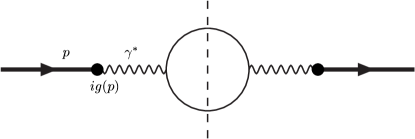
Figure 1: Feynman diagram for the one loop $e^{-}e^{+}$ contribution to the self-energy of a meson (solid line) with momeum $p$. All hadron information is contained in the transition form factor $g(p)$.

Applying standard QED covariant perturbation theory to evaluate the photon polarization tensor yields

$$\Pi_{\mu\nu}\simeq-e^{2}\int\frac{d^{4}q}{(2\pi)^{4}}\frac{{\rm Tr}(\gamma_{\mu}\not q\gamma_{\nu}(\not q+\not p))}{(q^{2}+i\epsilon)((q+p)^{2}+i\epsilon)}\ .$$ (5)

Note we have neglected the electron’s mass since it is a small effect. Related, Eq. (5) also represents the one loop $\mu^{-}\mu^{+}$ contribution in the zero mass limit and, as suggested by Table 1, this mass can also be neglected since $\Gamma_{\mu\mu}$ is essentially equal to $\Gamma_{ee}$ within experimental error. This conclusion is reinforced by $\Gamma_{\mu\mu}$ being randomly larger or smaller than $\Gamma_{ee}$, since phase space would indicate it to be smaller. Further, the decay width for $\Upsilon\to\tau^{-}\tau^{+}$ is also known and is compatible with the widths for $\mu^{-}\mu^{+}$ and $e^{-}e^{+}$ as well. The effect of the $\mu$ mass should be maximal for the $\rho$ and $\omega$ widths where the momentum of the outgoing particles is not as large. The relevant correction (see discussion below), $4m_{\mu}^{4}/p^{4}$, produces a $10\ \%$ suppression which is less than experimental error.

Table 1: Observed vector meson masses and leptonic widths. Partial widths estimated from the central PDG pdg value for the total width. The error quoted, affecting the last digit, corresponds to the uncertainty in the branching ratio alone.

State	$M(MeV)$	$\Gamma_{ee}(keV)$	$\Gamma_{\mu\mu}(keV)$
$\rho$	770	6.81(2)	6.9(4)
$\omega$	783	0.60(2)	0.76(25)
$\phi$	1019	1.26(2)	1.22(9)
$J/\psi$	3097	5.2(1)	5.1(9)
$\psi(2S)$	3686	2.1(1)	2.1(3)
$\Upsilon$	9460	1.32(5)	1.30(3)
$\Upsilon(2S)$	10023	0.52(3)	0.58(9)

Performing the Dirac traces in Eq. (5) and employing the tensor integral relations for a scalar function $F$

$$\int q_{\mu}q_{\nu}F(q,p)\ d^{4}q = \frac{g_{\mu\nu}}{3}\int[q^{2}-\frac{(q\!\cdot\!p)^{2}}{p^{2}}]F\ d^{4}q$$ (6)

$$+ \frac{p_{\mu}p_{\nu}}{3p^{4}}\int[4(q\!\cdot\!p)^{2}-p^{2}q^{2}]F\ d^{4}q$$

$$\int q_{\mu}F\ d^{4}q = \frac{p_{\mu}}{p^{2}}\int q\!\cdot\!pF\ d^{4}q$$ (7)

one can obtain scalar integral expressions. Since we only require the imaginary (finite) part of the $\Sigma$ self-energy, we can ignore all real (known to be UV divergent) contributions. For example, we suppress the tadpole integral

$$\int\frac{d^{4}q}{(2\pi)^{4}}\frac{q^{2}}{(q^{2}+i\epsilon)((q+p)^{2}+i\epsilon)}=\int\frac{d^{4}q}{(2\pi)^{4}}\frac{1}{(q+p)^{2}+i\epsilon}\to 0$$

in this calculation (the real, mass shifts from lepton loops are totally negligible). After some manipulation

$${\rm Im}\ (i\ \Pi(p^{2}))=-\frac{4e^{2}}{3}\ {\rm Im}\ (i\ J)$$ (8)

where $J$ is the standard massless boson loop integral

$$J=\int\frac{d^{4}q}{(2\pi)^{4}}\frac{1}{(q^{2}+i\epsilon)((q+p)^{2}+i\epsilon)}\ .$$ (9)

The $q_{0}$ integral is easily performed in the complex plane and the remaining integral can be obtained with the substitution

$$\frac{1}{E-E_{r}-i\epsilon}\to 2\pi i\delta(E-E_{r})\ .$$

The result (identical to using Fermi’s golden rule) is

$${\rm Im}(i\ J)=-\frac{1}{16\pi}$$

giving the theoretical leptonic width

$$\Gamma=2\ {\rm Im}{\Sigma}(M^{2})=\frac{2\alpha_{EM}}{3M^{2}}g^{2}(M^{2})\ .$$ (10)

For completeness, the correction to Eq. (10) due to a non-zero lepton mass, $m$, in the polarization tensor is obtained peskin by replacing the explicit fine structure constant with

$$\alpha_{EM}\to\alpha_{EM}\sqrt{1-\frac{4m^{2}}{q^{2}}}\left(1+\frac{2m^{2}}{q^{2}}\right)\simeq\alpha_{EM}\left(1-\frac{4m^{4}}{q^{4}}\right)\ .$$ (11)

3 RPA Leptonic Widths

To evaluate $\Gamma_{ee}$ in the RPA we need to calculate the transition form factor $g(p)$. As indicated in Fig. 2 there are both meson and quark loop contributions.

Figure 2: Diagrams for the transition form factor $g(p)$: (a) hadron decay and rescattering before annihilation; (b) direct quark-antiquark annihilation.

In the next section we show that the quark-antiquark annihilation, Fig. 2b, is the dominant process with contribution in the RPA given by

$$g=\frac{eq}{\langle\Omega\arrowvert\Omega\rangle}\langle\Omega\arrowvert\left[\Psi^{\dagger}(0)\alpha^{i}\Psi(0),V^{i\dagger}\right]\arrowvert\Omega\rangle_{\rm RPA}$$ (12)

where $\Psi$ is the quark field operator and $q$ the (fractional) quark charge in electron units. The RPA vector meson creation operator with spin projection $i$ is denoted by $V^{i\dagger}$ and contains creation and annihilation parts

$$V^{i\dagger}=X^{i}_{\alpha\beta}B^{\dagger}_{\alpha}D^{\dagger}_{\beta}-Y^{i}_{\alpha\beta}B_{\alpha}D_{\beta}$$ (13)

with all remaining quantum numbers represented by $\alpha$ and $\beta$. For $J^{PC}=1^{--}$ states there are $S$ and $D$ wavefunction components

$$X_{S}^{i}({\bf k}) = \frac{\delta^{ab}}{\sqrt{N_{c}}}\frac{1}{\sqrt{4\pi}}\frac{\sigma^{i}i\sigma_{2}}{\sqrt{2}}X_{S}(k)$$ (14)

$$Y_{S}^{i}({\bf k}) = \frac{\delta^{ab}}{\sqrt{N_{c}}}\frac{-1}{\sqrt{4\pi}}\frac{i\sigma_{2}\sigma^{i}}{\sqrt{2}}Y_{S}(k)$$ (15)

$$X_{D}^{i}({\bf k}) = \frac{\delta^{ab}}{\sqrt{N_{c}}}\frac{1}{\sqrt{4\pi}}\frac{3}{2}\left(\hat{\bf k}\!\cdot\!{\bf\sigma}\hat{k}^{i}-\frac{1}{3}\sigma^{i}\right)i\sigma_{2}X_{D}(k)$$ (16)

$$Y_{D}^{i}({\bf k}) = \frac{\delta^{ab}}{\sqrt{N_{c}}}\frac{-1}{\sqrt{4\pi}}i\sigma_{2}\frac{3}{2}\left(\hat{\bf k}\!\cdot\!{\bf\sigma}\hat{k}^{i}-\frac{1}{3}\sigma^{i}\right)Y_{D}(k)$$ (17)

with color indices $a,b,c$ and $N_{c}=$ 3. The normalization condition

$$\frac{\langle\Omega\arrowvert\left[V^{i},V^{i\dagger}\right]\arrowvert\Omega\rangle}{\langle\Omega\arrowvert\Omega\rangle}=1$$ (18)

reduces to

$$\frac{1}{(2\pi)^{3}}\int_{0}^{\infty}k^{2}dk\left(\arrowvert X_{S}(k)\arrowvert^{2}+\arrowvert X_{D}(k)\arrowvert^{2}-\arrowvert Y_{S}(k)\arrowvert^{2}-\arrowvert Y_{D}(k)\arrowvert^{2}\right)=1\ .$$ (19)

The scalar wavefunctions are solutions to coupled integral equations resulting from the RPA diagonalization of the Coulomb gauge Hamiltonian weall . A state-of-the-art QCD confining potential with scale (string tension or gluon generated mass) connected to $\Lambda_{\rm QCD}$ was used along with a transverse gluon exchange hyperfine interaction, essentially a Yukawa potential, supported by recent lattice results langfeld , with a range parameter chosen to adjust the mass-spectra.

In evaluating Eq. (12) we note that spin is conserved in the vector meson-photon transition (diagonal coupling). Rotational invariance permits summing over the three spin components if we divide by 3. The resulting RPA $g$ is then

$$g = \frac{eq\sqrt{8\pi N_{c}}}{3}\int_{0}^{\infty}\frac{k^{2}dk}{(2\pi)^{3}}\Big{[}(X_{S}(k)-Y_{S}(k))(2+\sin\phi(k))$$ (20)

$$-\sqrt{2}(1-\sin\phi(k))(X_{D}(k)-Y_{D}(k))\Big{]}\ .$$

Note that the RPA leads to an expression of the form given by Eq. (1) since $\Gamma\propto g^{2}$, and in the non-relativistic limit

$$g\to eq\sqrt{8\pi N_{c}}\int_{0}^{\infty}\frac{k^{2}dk}{(2\pi)^{3}}X_{S}(k)$$ (21)

because $sin\ \phi(k)$, the BCS vacuum angle (solution of the gap equation for the same Hamiltonian), approaches unity

$$\sin\phi(k)=\frac{M_{q}(k)}{\sqrt{k^{2}+M_{q}(k)^{2}}}\simeq 1$$ (22)

for large running quark mass and the $Y$ function can be neglected in the same limit. Finally the Fourier-transformed wavefunction is

$$\psi(0)\propto\int e^{ik\!\cdot\!0}\frac{d^{3}k}{(2\pi)^{3}}\frac{X_{S}(k)}{\sqrt{4\pi}}\ .$$ (23)

The effective charge factors, $q^{2}\rightarrow<q^{2}>$, for the various quark flavors necessary for our width calculation are listed in Table 2. This is the origin of the order of magnitude suppression of the $\omega$ width relative to the $\rho$. We work in the exact isospin limit.

Table 2: Quark charge factors $\langle q^{2}\rangle$.

State	Flavor			$\langle q^{2}\rangle$
$\Upsilon$	$b\bar{b}$			$\frac{1}{9}$
$J/\psi$	$c\bar{c}$				$\frac{4}{9}$
$\phi$	$s\bar{s}$			$\frac{1}{9}$
$\rho$	$\frac{u\bar{u}+d\bar{d}}{\sqrt{2}}$				$\frac{1}{2}$
$\omega$	$\frac{u\bar{u}-d\bar{d}}{\sqrt{2}}$			$\frac{1}{18}$

Combining Eqs. (10) and (20) yields the final expression for the RPA widths. The numerical predictions for both meson masses and widths are listed in Table 3. The predicted masses are only in rough agreement since a fit was not attempted (the quark masses were not fine-tuned). To avoid compounding errors, the physical meson masses were used in Eq. (10) except for the unknown $\phi(1880)$ where the model mass is adopted. Given the large errors in the measured lepton widths this should be a minor concern. For comparison, two other theoretical calculations isgur ; ebert are also presented. It is noteworthy that our few parameter approach provides a description which is comparable to these multi-parameter models.

Table 3: Experimental and theoretical vector meson widths. Also listed are two other calculations, marked ¹ (Godfrey and Isgur isgur $S$-$D$ wave results without mixing) and ² (Ebert, Faustov and Galkin ebert ).

State	Exp. $M(MeV)$	Calculated	Exp. $\Gamma_{e^{-}e^{+}}(keV)$	Calculated	Other works
$\rho$	770	795	6.85	4.7	$6.87^{1}$
$\omega$	782	795	0.60(2)	0.50	$0.85^{1}$
$\phi$	1019	1005	1.26(2)	1.1	$2.75^{1}$
$\omega$	1420	1420	$0.1(1)^{\dagger}$	0.18	$0.046^{1}$
$\rho$	1450(25)	1420	-	1.5	$0.45^{1}$
$\omega$	1650(25)	1620	-	0.23	$0.013^{1}$
$\phi$	1680(25)	1670	$0.5(10)^{\dagger}$	0.21	$0.27^{1}$
$\rho$	1700	1520	$3.5(5)^{\dagger}$	2.0	$0.14^{1}$
$\phi$	-	1790	-	0.45-0.55	$0.06^{1}$
$J/\psi$	3097	3130	5.2(1)	3.8	$9.9^{1}$, $5.4^{2}$
$\psi$	3686	3681	2.2(2)	2.0	$3.3^{1}$,$2.4^{2}$
$\psi$	3770	3695	0.26(4)	0.68	$0.10^{1}$
$\psi$	4040	4140	0.75(15)	1.7	$1.8^{1}$
$\psi$	4160(20)	4150	0.77(23)	0.56
$\psi$	4415(6)	4535	0.47(10)	0.26
$\Upsilon$	9460	9460	1.32(5)	0.45	$1.4^{1}$,$1.3^{2}$
$\Upsilon$	10023	9870	0.52(3)	0.35	$0.65^{1}$, $0.5^{2}$
$\Upsilon$	10365	9921	$0.5(1)^{\ddagger}$	0.0003	$0.45^{1}$
$\Upsilon$	10580	10190	$0.32(3)^{\S}$	0.29	$0.34^{1}$

^†our estimate   ^‡ $\mu^{+}\mu^{-}$ width (roughly equal)  ^§ recently reported by BaBar babar

Finally, we can relate our form factor parameter, $g$, to the standard vector meson leptonic decay constant, $f_{V}$, defined by

$$\Gamma_{e^{-}e^{+}}=\frac{4\pi}{3}\alpha^{2}_{EM}M_{V}f_{V}^{2}\ .$$ (24)

Comparing to Eq. (10) yields

$$g=ef_{V}\sqrt{\frac{M_{V}^{3}}{2}}$$ (25)

with mass dimension consistent with Eqs. (19) and (20). In representing the widths from Ref. isgur we use their $f_{V}$ values and again available physical meson masses. Combining the different models it is clear that we have a reasonable theoretical understanding of vector meson dileptonic decay.

4 Mesons with Broad Hadronic Widths

For vector meson decay to a particle-antiparticle hadron pair, annihilation to a virtual photon is possible which also contributes to the total lepton width. In this section we will demonstrate that such rescattering corrections are small in comparison with the intrinsic quark-antiquark annihilation contribution. A typical example of a broad vector meson width is the $\rho\rightarrow\pi\pi$. We assume that the true eigenstate of the full QCD Hamiltonian also contains a two-pion wavefunction component

$$\arrowvert\rho\rangle=\alpha\arrowvert q\bar{q}\rangle+\beta\arrowvert\pi\pi\rangle+\!\cdot\!\!\cdot\!\!\cdot\!$$ (26)

with $\arrowvert\beta\arrowvert<1$. We have previously calculated the decay of the $q\bar{q}$ component into $e^{-}e^{+}$ and now proceed to estimate the contribution from the $\arrowvert\pi\pi\rangle$ term.

In principle this higher Fock-space wavefunction component could be computed from the same model Hamiltonian employed in the $q\bar{q}$ two-body sector since it is field-theory based. However this is a challenging calculation involving four relativistic particles and chiral symmetry. Although a formalism has been developed pcfmrs to treat this problem, for an order of magnitude estimate we instead implement a simple model wavefunction and adopt the following ansatz for the $V=\rho$ two-pion component

$$V^{i\ a\dagger}(p=(M_{V},{\bf 0}))\arrowvert\Omega\rangle = \int\frac{d^{3}k}{(2\pi)^{3}}\frac{\sqrt{3}\hat{k}^{i}}{\sqrt{4\pi}}\frac{\epsilon^{abc}}{\sqrt{2}}\frac{\Gamma_{\pi\pi}/2}{M_{V}-2E_{k}-i\Gamma_{V}/2}$$ (27)

$$\sqrt{\frac{2(2\pi)^{3}}{2M_{V}kE_{k}}}\frac{1}{\sqrt{2}}\pi^{b\dagger}_{\bf k}\pi^{c\dagger}_{-{\bf k}}\arrowvert\Omega\rangle\ .$$

Here $E_{k}=\sqrt{M_{\pi}^{2}+k^{2}}$, $\Gamma_{V}$ is the total $V$ width and $\Gamma_{\pi\pi}$ is the width for the $\pi^{+}\pi^{-}$ decay. The indices $a,b$ and $c$ now denote charge states. This wavefunction is inspired by the scattering amplitude for $h^{+}h^{-}$ hadrons coupled to angular momentum 1 near a resonance described by the Breit-Wigner amplitude

$$a_{1}(s)=-\frac{M_{V}\Gamma_{hh}/2}{s-M_{V}^{2}+iM_{V}\Gamma_{V}}$$ (28)

or in the $V$ rest frame with $E=M_{V}+i\Gamma_{V}/2$

$$a_{1}(E)=\frac{\Gamma_{hh}/2}{M_{V}-E-i\Gamma_{V}/2}=\frac{i\Gamma_{hh}}{2\Gamma_{V}}\ .$$ (29)

The normalization is given by

$$\frac{\langle\Omega\arrowvert\ \left[V^{i\ a},V^{j\ a^{\prime}\dagger}\right]\arrowvert\Omega\rangle}{\langle\Omega\arrowvert\Omega\rangle}=\delta^{aa^{\prime}}\delta^{ij}(2\pi)^{3}\delta^{3}(0)\ {\cal N}^{2}$$ (30)

where the factor ${\cal N}^{2}$ (smaller than unity) is

$${\cal N}^{2}=\frac{1}{2M_{V}}\int_{2m_{\pi}}^{\infty}dE\frac{\Gamma^{2}_{\pi\pi}/4}{(E-M_{V})^{2}+\Gamma_{V}^{2}/4}$$ (31)

and represents the probability of finding a pion pair with relative momentum given by the Breit-Wigner distribution. This determines the $\beta$ coefficient above. This normalization also represents the number of pion pairs per $\rho$ under the Breit-Wigner curve.

The pion pair annihilation to a photon involves the electromagnetic current

$$j^{i\ a}(0)=i\epsilon^{abc}\pi^{b\dagger}(0)\partial^{i}\pi^{c\dagger}(0)$$ (32)

taken bare as all pion rescattering effects are already included in the Breit-Wigner distribution. The pion field at the origin can be expressed in terms of the pion momentum operator

$$\pi^{b}(0)=\int\frac{d^{3}q}{(2\pi)^{3}}e^{i\vec{q}\!\cdot\!\vec{0}}\pi^{b}_{\bf q}\frac{1}{\sqrt{2E_{q}}}\ .$$ (33)

The hadronic transition coefficient is then

$$g=eq\frac{1}{3}\sum_{a}\frac{1}{3}\sum_{i}\frac{\langle\Omega\arrowvert j^{i\ a}(0)V^{i\ a\dagger}\arrowvert\Omega\rangle}{\langle\Omega\arrowvert\Omega\rangle}$$ (34)

where the charge factor is now 1 as both hadrons carry one electron unit and spin and isospin are averaged over. The straightforward computation yields

$$g=eq\frac{\sqrt{4\pi}}{\sqrt{3(2\pi)^{3}M_{V}}}\int_{0}^{\infty}\frac{k^{5/2}dk}{E_{k}^{3/4}}\frac{\Gamma_{\pi\pi}/2}{M_{V}-2E_{k}-i\Gamma_{V}/2}\ .$$ (35)

The imaginary part of the integral is finite, but the real part diverges linearly with increasing momentum cut-off $\Lambda$. This reflects short range physics and the need for a counterterm in the vector current of Eq. (32). Since the “contact” part of the decay has been calculated using the RPA, the counterterm coefficient (or simply the cutoff in the integral) could be fixed by the difference between the physical and RPA lepton widths. But this generates an unnaturally large cutoff which is not expected for pions with energies comparable to the mass $V$, i.e. pion pairs with energies beyond a GeV from the resonance should not appreciably contribute. A third way to regularize the integral is to allow for an energy-dependent width that localizes the integrand. In principle all three ways are equivalent and we therefore use the simple cut-off regularization with parameter $\Lambda$. The results for the $e^{-}e^{+}$ widths corresponding to the three lowest $\rho$ states are presented in Table 4 for different model parameters. The momentum cut-off is listed dimensionlessly, $(\Lambda-M_{V})/\Gamma_{V}$, in terms of the $V$ mass and width.

Table 4: Contribution to $\Gamma_{V\to e^{-}e^{+}}$ from $\pi\pi$ pion rescattering.

$M_{V}\ (MeV)$	$\Gamma_{V}\ (MeV)$	$\Gamma_{\pi\pi}\ (MeV)$	$\cal N$	$(\Lambda-M_{V})/\Gamma_{V}$	$\Gamma_{ee}\ (keV)$
700	150	150	0.38	5	0.068
700	150	150	0.38	10	0.156
1465	350	100	0.12	5	0.028
1465	350	100	0.12	10	0.064
1700	240	80	0.11	5	0.0070
1700	240	80	0.11	10	0.014

Note that the rescattering contribution to the electron-positron widths are suppressed relative to direct quark-antiquark annihilation by an order of magnitude. With this estimate and the present experimental width precision, the RPA calculation appears to provide a sufficient description without the need for rigorously including hadron final-state interactions. Further, rescattering effects for other meson decays can be even smaller. For example, in odd $G$ parity $\omega$-type meson decays to three or more (odd) particle states, the final state mesons are very unlikely to recombine and annihiliate to a photon. Also the $\phi$ and several other quarkonium states have narrow widths because they are near or below hadronic decay thresholds. Finally, the $\phi(1680)$ has an $\omega$-like decay pattern with dominant $K^{*}K$ decay products which cannot directly annihilate into a single photon.

5 Towards baryonium

The short-ranged (weak) $NN$ interaction, $V_{NN}$, can only produce a single bound state, the deuteron. In contrast, for the $N\bar{N}$ system the stronger $V_{N\bar{N}}$ interaction obtained from $V_{NN}$ using $G$ parity can support several bound states. However, because of annihilation and also mixing and decay to other baryon number zero hadrons (mesons), it has long been believed that baryonium states, if found, would be quite broad. Significantly, BES has reported bes a dramatic narrow enhancement in the decay $J/\psi\to\gamma p\bar{p}$ but not in $J/\psi\to\pi_{0}p\bar{p}$. This indicates the possibility of an $I=0$, as opposed to $I=1$, bound state not far below threshold kerbikov . The quantum numbers of this state are likely to be either $J^{PC}=0^{-+}$ or $0^{++}$. If it is a pseudoscalar state, it cannot be explained in a $q\bar{q}$ model since the expected excited $\pi$ and $\eta$ states in this region have already been identified as the $\pi(1800)$ and $\eta(1760)$.

The baryonium interpretation of this resonance suggests the pseudoscalar assignment corresponding to para baryonium (nucleon and antinucleon spins antiparallel) which, in turn, implies a partner, ortho baryonium, with spins alligned having total $J^{PC}=1^{--}$. A similar state is also suggested by the observed low-energy proton timelike form factor behavior as well as by a $J^{PC}=1^{--}$ resonance prediction using Vector Meson Dominance williams just below the $e^{-}e^{+}\rightarrow p\bar{p}$ threshold. Further, a state, with mass $1870(10)\ MeV$ and width $10(5)\ MeV$, has also been reported by the Fenice collaboration fenice in $e^{-}e^{+}$ production but awaits confirmation. Another discrepancy with expected phase-space is reported abe in $B\to\bar{p}pK$.

Since baryonium has conventional meson quantum numbers, it is difficult to disentangle from $q\bar{q}$ and $2q$-$2\bar{q}$ states. In particular, quark models predict numerous four-quark states that likely overlap forming a hadron continuum. The best prospect for observing baryonium states would be if they had narrow widths (possibly due to significant quark recombination) and non-strange decay products near the $N\bar{N}$ threshold. Such states are predicted by the Resonating Group Method ribeiro . Because the BES and FENICE resonances both have widths of order $10\ MeV$, Coulombic baryonium states bound by just QED are unlikely to be observed since these would have very narrow leptonic widths given by

$$\Gamma_{B\to e^{-}e^{+}}=\frac{4}{3}\alpha_{EM}^{5}M_{p}/(2n)$$ (36)

that are of order $10\ eV$. Instead, we would anticipate one ortho and one para baryonium level each with a typical width of order 10 MeV.

Experimental information above threshold should be regarded more cautiously. As recently discussed bugg , steep peaks in the nucleon timelike form factors and $J/\psi$ decays could be simple threshold cusp effects. Consequently, baryonium claims should focus below threshold on isolated peaks or dips in an observable like the unconfirmed dip at 1870 MeV in the total $e^{-}e^{+}$ annihilation cross section fenice .

6 $\phi(1880)$

Since ortho baryonium is a vector state it should be readily accessible with new high energy and luminosity $e^{-}e^{+}$ colliders, such as the envisioned DA$\Phi$NE upgrade to 2 $GeV$ dafne . In this energy region, the most likely hadron to be observed is the excited $\phi$ meson, a combination of $2S$ and $1D$ waves, with mass $1880\ MeV$ predicted by Isgur and Godfrey and $1790\ MeV$ in our RPA model. As listed in Table 3, our calculated $e^{-}e^{+}$ width for this state is about half a $keV$.

We can also phenomenologically estimate this width using known data and flavor symmetry. Recall Weinberg’s first sum rule

$$\frac{1}{3}M_{\rho}\Gamma_{\rho\to e^{-}e^{+}}=M_{\omega}\Gamma_{\omega\to e^{-}e^{+}}+M_{\phi}\Gamma_{\phi\to e^{-}e^{+}}$$ (37)

which appears reasonable desy since the left and right sides of this equation are 1.758 and 1.754 $MeV^{2}$, respectively. Assuming ideal mixing for the $\omega$-$\phi$ system, we obtain

$$2M_{\rho}\Gamma_{\rho\to e^{-}e^{+}}=9M_{\phi}\Gamma_{\phi\to e^{-}e^{+}}=18M_{\omega}\Gamma_{\omega\to e^{-}e^{+}}$$ (38)

which is satisfied to within $30\ \%$ ($10.5,\ 11.6,\ 8.4\ MeV^{2}$, respectively). Combining Eqs. (37) and (38) with the known pdg relative branching ratio

$$\frac{\Gamma_{\rho(1700)\to e^{-}e^{+}}\Gamma_{\rho(1700)\to 2(\pi\pi)}}{\Gamma_{\rho(1700)\to{\rm all}}}$$

we obtain the estimates, $\Gamma_{\rho(1700)\to e^{-}e^{+}}=3.5(0.5)\ keV$, $\Gamma_{\phi(1880)\to e^{-}e^{+}}=0.7(3)\ keV$ and $\Gamma_{\omega(1650)\to e^{-}e^{+}}=0.4(2)\ keV$. These are somewhat larger but still in agreement with our model calculations. Therefore, in searching for $J=1$ baryonium candidates below the $N{\bar{N}}$ threshold, there may be a $\phi(1880)$ state with $\Gamma_{ee}$ about half a $keV$ which should be distinguishable by its kaon decay modes.

7 Outlook

Recent claims have again raised the question concerning the existence of baryonium states but more solid information is needed near the $N{\bar{N}}$ threshold. The upgrade of DA$\Phi$NE to the $2\ GeV$ range will provide a good opportunity for further searches. A possible fruitful strategy would be to focus on $e^{-}e^{+}$ annihilation into an even number of pions in isoscalar $1^{--}$ states. Resonances, although not narrow, are anticipated and there are structure precursors baldini from other experiments. By extracting the leptonic widths, the missing $\phi$ state below 2 $GeV$ should be found and we predict its lepton width to be around half a $keV$. Its hadron width should be similar to the $\omega(1650)$, about 200 $MeV$. Any other observed vector state is a candidate for ortho baryonium.

This work is supported by grants FPA 2000-0956, BFM 2002-01003 (MCYT, Spain) and DE-FG02-97ER41048 (US Department of Energy) and has been commissioned for the “Encuentro de Física Fundamental Alberto Galindo” meeting at Univ. Complutense, November, 2004. The authors are grateful to the workshop organizers and congratulate Professor Galindo on his Iubilaeum.

References

- (1) Appelquist T et al. (1975) Phys. Rev. Lett. 34:365
- (2) Schnitzer H J (1975) Phys Rev D 13:74; Van Royen R, Weisskopf V F (1967), Nuovo Cimento 50:617; (1967) 51:583
- (3) Godfrey S Isgur N (1985) Phys Rev D 32:189
- (4) Llanes-Estrada F J Cotanch S R (2000) Phys Rev Lett 84:1102
- (5) Llanes-Estrada F J Cotanch S R Szczepaniak A P Swanson E S Phys Rev C in press arXiv:hep-ph/0402253; (2003) arXiv:hep-ph/0311246 proceedings EPS HEP conference, Aachen. See also R. Alkofer and P.A. Amundsen, Nucl. Phys. B306, 305 (1988) for related work.
- (6) Bai J Z et al. (2003) Phys Rev Lett 91:022001
- (7) Gao C-S Zhu S-L arXiv:hep-ph/0308205
- (8) Kerbikov B Stavinsky A Fedotov V arXiv:nucl-th/0310060
- (9) Hagiwara et al. [Particle Data Group PDG] (2002) Phys Rev D 66:010001
- (10) Peskin M E Schroeder D V (1995) An introduction to quantum field theory. Addison Wesley
- (11) Langfeld K Moyaerts L arXiv:hep-lat/0406024 C. Feuchter and H. Reinhardt, work in preparation.
- (12) Ebert D Faustov R N Galkin V O (2000) arXiv:hep-ph/0304227. For the full model account see (2000) Phys Rev D 62:034014. Also Eichten E Quigg J C (1995) Phys Rev D 52:1726 arXiv:hep-ph/9503356
- (13) Aubert B et al. [BABAR Collaboration] arXiv:hep-ex/0405025
- (14) Bicudo P Cotanch S R Llanes-Estrada F J Maris P Ribeiro E Szczepaniak A (2002) Phys Rev D 65:076008
- (15) Williams R Cotanch S R (1996) Phys Rev Lett 77:1008; (2002) Phys Lett B 549:85-92
- (16) Antonelli A et al. (1996) Phys Lett B 365:427
- (17) Abe K et al. (2002) Phys Rev Lett 88:181803; Abe K et al. (2002) Phys Rev Lett 89:151802; Bai J Z et al. (2003) Phys Rev Lett 91:022001
- (18) Ribeiro J E T (1980) Z Phys C 5:27
- (19) Bugg D V arXiv:hep-ph/0406293
- (20) See conference proceedings eConf C0309101
- (21) Becker U et al. (1968) Phys Rev Lett 21:1504
- (22) Baldini R private communication