On the reaction $\gamma d\!\to\!\pi^{0}d$ near the threshold of $\eta$ production

Abstract

We consider the reaction $\gamma d\!\to\!\pi^{0}d$ in a wide energy range around and above the $\eta$-meson photoproduction threshold at backward CM angles of the outgoing pion. Our theoretical analysis is essentially motivated by the recent measurements of the CLAS Collaboration at Jefferson Lab, where this kinematical region of the reaction has been thoroughly studied for the first time and a cusps in the energy dependence of the differential cross section in the region of $E_{\gamma}\sim 600-800$ MeV has been observed. Our preliminary and qualitative analysis, based on single- and double-scattering diagrams, shows that the observed structure can be explained by the contribution of the double-scattering diagram with intermediate production of the $\eta$ meson. The effect, to a considerable extent, is formed due to the contribution of $N(1535)$ resonance to the amplitudes of subprocesses on the nucleons.

I Introduction

The reaction of coherent photoproduction of the $\pi^{0}$ meson on the deuteron

$$\gamma d\!\to\!\pi^{0}d$$ (1)

has recently been studied CLAS at Jefferson Lab using the CLAS detector. The experiment was carried out in a wide range of photon energies $E_{\gamma}=0.5-2.0$ GeV at large CM scattering angles of the outgoing pions. A new phenomenon was observed.

The process of pion photoproduction on the nucleon $\gamma p\!\to\!\pi N$ has been theoretically investigated over a long period of time (see, for example, Refs.  Walker ; Moor ; Garc ; Drech ). The reaction (1)  on the deuteron, has been also considered in a number of papers Garc1 ; Kamal . During the last years, the $\eta$-photoproduction processes have also been actively studied (see, for example, Refs.  Knoch ; Benme for $\gamma p\!\to\!\eta p$, Kamal ; Ritz for $\gamma d\!\to\!\eta d$, and Benn for $\eta$ photoproduction on light nuclei).

The study of the meson-photoproduction processes on a deuteron target provides information about the underlying reaction mechanisms on few-body systems. Our project has been motivated by a special interest in the role of intermediate particles in reaction (1).

In the 1970’s, the contribution of intermediate particles and resonances to the differential cross section in the backward $\pi d$ elastic scattering was theoretically discussed in Ref. Kond . It has been predicted that the contribution of intermediate particles, formed in a two-step process, should manifest itself a cusp in the energy dependence of the backward differential cross section around the corresponding thresholds. Such an effect, associated with intermediate $\eta$-meson production, was confirmed by several independent measurements of backward $\pi d$ elastic scattering pide .

The preliminary CLAS photoproduction data CLAS give for first time clear evidence for the intermediate $\eta$-meson effect. A cusp in the region around the $\eta$ photoproduction threshold, $E_{\gamma}\sim 600-800$ MeV, is visible in the energy dependence of the differential cross section at large CM scattering angles, $\cos\theta<-0.6$. The observed effect becomes more pronounced as the scattering angle increases. This behavior was also seen in a previous measurement of reaction (1) Iman in which a small structure was observed in the excitation function the differential cross section at $\cos\theta=-0.64$ (the maximum scattering angle of this experiment). Reaction (1) was also theoretically considered earlier (see, for example, Ref. Garc ) in the framework of single- and double-scattering approach without consideration of the intermediate $\eta$ meson. A reasonable theoretical description of the previous data Iman was achieved without the necessity of inclusion of the “$\eta$ effect” Garc at low momentum transfer.

The aim of the present paper is the theoretical study of reaction (1) at large pion production angles. Our principal interest is the contribution of the intermediate $\eta$ meson to the differential cross section and whether it can explain the structure in the differential cross section that has been observed in a recent CLAS experiment CLAS . We shall use the standard approach based on single- and double-scattering amplitudes. The main contribution to the total amplitude at large angles is expected to come from the double-scattering terms. We shall consider photon energies far from the $\pi d$ threshold, say $500<E_{\gamma}<1000$ MeV, where the influence of the intermediate $N(1535)$ resonance and the $\eta$ meson effect should be important, and it is possible to neglect the excitation of the $\Delta(1232)$ isobar in the intermediate state. Thus, we construct the total reaction amplitude from terms, expected to be essential, with approximate values of the parameters. In this paper, while we do compare our predictions with the data qualitatively and present all the details of our treatment, we do not attempt a detailed description of the CLAS data; we leave this task for forthcoming papers from the CLAS Collaboration.

This paper is organized as follows. In Section II, we derive the expressions for different terms of the amplitude of  reaction (1) in a diagrammatical approach. In Subsection  II.1, we briefly discuss the main contributions to the reaction amplitude and introduce the notation that we use. In Subsections  II.2 and  II.3, we give gauge-invariant expressions for the resonance and VME contributions to the elementary amplitudes on the nucleon. These results are used in Subsections II.4 and  II.5 to obtain single- and double-scattering amplitudes of reaction (1), respectively. In Section III, we present the numerical results. In Subsection III.1, we study the influence of the “non-static” corrections that are taken into account in the double-scattering amplitude with intermediate $\eta$ production. In Subsection  III.2, we discuss our numerical results for the differential cross section (its energy behavior at several values of $\cos\theta$) of reaction (1) with backward $\pi^{0}$ production. The conclusion is presented in Section IV. In Appendices A,  B,  C, and  D, we calculate the the integrals and some other expressions, used to derive the single- and double-scattering amplitudes of reaction (1).

II Formalism

II.1 Diagrams and notation

The diagrams for single- and double-scattering amplitudes $M_{(1)}$ and $M_{(2)}$ of reaction (1) are shown in Figs. 1a and 1b, respectively. The notation for the four-momentum vectors of the initial, intermediate, and final particles are given in this figure. The vertices marked by “$i\,$” or “$j\,$” correspond to the elementary amplitudes of the subreactions on the nucleons, and indices “$i\,$”, “$j\,$” specify the contributions to the elementary amplitudes considered below. In Fig. 1b, the notation “$h$” stands for the intermediate meson. Hereafter, we shall consider only diagrams with $h=\pi$ or $\eta$.

The elementary photoproduction amplitude $\gamma N\!\to\!hN$ is usually constructed as a sum of Born, vector-meson-exchange (VME), and resonance terms Garc ; Drech ; Benme . The Born amplitudes correspond to a set of tree diagrams with $N\!Nh$ coupling and all possible couplings with a photon, summed by a contact $\gamma\pi N\!N$-coupling term. It is known that the total Born amplitude satisfies gauge invariance (see Ref.  Garc and references therein). Using Born amplitudes for subprocesses in reaction (1) on the deuteron, one encounters the problem how to get the total gauge-invariant amplitude. The problem comes from nucleon off-shell effects, and the way to solve it is discussed, for example, in Ref. Kamal (see also references therein). However in our analysis, we shall neglect Born terms in the kinematical region of reaction under study.

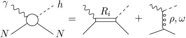
Figure 2: Diagrams of meson photoproduction on the nucleon (resonance and VME contributions).

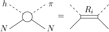
Figure 3: Diagrams of meson-nucleon binary reactions (resonance contributions).

The resonance and VME terms in the photoproduction amplitude are shown graphically in Fig.  2, where VME terms are calculated via $\rho$ and $\omega$ exchanges  Garc ; Benme . The “meson-meson” $hN\!\to\!\pi N$ amplitudes are written through resonance contributions (Fig. 3). The main contribution from an intermediate $\eta$ meson to the cross section of reaction (1) is expected from the double-scattering diagram in Fig.  1b ($h=\eta$), with the $N(1535)$ excitation in both blocks of the diagram due to the large partial width of the decay $N(1535)\!\to\!\eta N$. Several nucleon resonances  PDG are coupled to the $\pi N$ system. Also, the couplings of $N(1535)$, $N(1440)$ , and $N(1520)$ to the $\eta N$ system Garc1 ; Ritz ; Benn are often used in the production amplitudes. However in our qualitative analysis, we shall limit the resonance parts of the elementary amplitudes (Figs. 2 and  3) to the contributions of the $N(1535)$ in the $\pi N$ and $\eta N$ channels and the $N(1440)$ in the $\pi N$ channel. We do not include the contribution of the $\Delta(1232)$ isobar since the considered energies are far above the $\Delta(1232)$ region.

Let us write the total amplitude $M_{\gamma d}$ of reaction (1) as

$$M_{\gamma d}=M_{(1)}+M_{(2)}\,,{~{}~{}~{}~{}}M_{(1)}=\sum_{i}M_{i}\,,{~{}~{}~{}~{}}M_{(2)}=\sum_{i,\,h,\,j}M_{ihj}\,,$$ (2)

where $h\!=\!\pi,\eta$ and index $i=1,2,\omega$, and $\rho$ (the same for $j$) stands for $N(1535)$, $N(1440)$, $\omega$- and $\rho$-exchange for the elementary subprocesses, respectively. Note that $\rho$-exchange term in the single-scattering amplitude $M_{(1)}$ is forbidden by isotopic arguments. We shall use standard normalizations for the amplitudes, corresponding to the following expression of the differential cross section for a binary reaction:

$$\frac{d\sigma}{d\Omega_{{}_{CM}}}=\frac{k}{64\pi^{2}s_{\,}q}\,\overline{|M|^{2}}\,.$$ (3)

Here, $\overline{|M|^{2}}$ is the square of the total amplitude, averaged (summed) over the polarizations of the initial (final)particles; $s$ is the square of the total CM energy; and $q$ and $k$ are the relative 3-momenta of the initial and final state particles. Below, we use the following notation: $\varphi_{1,2}$ ($\chi_{1,2}$) are Pauli spinors (isospinors) for the initial and final nucleons in the elementary reactions or for the nucleons in the deuteron and $\varphi^{+}\varphi\!=\!1$ ($\chi^{+}\chi\!=\!1$); $\breve{a}\equiv({\bf a}\mbox{\boldmath$\sigma$})$, where $a$ is any 3-vector and $\sigma$ is a 3-vector from the Pauli spin matrices.

In Subsections  II.2 and  II.3, we give gauge-invariant expressions for the elementary amplitudes on the nucleon, notations for coupling constants etc., that will be used for the total amplitude $M_{\gamma d}$ in Subsections II.4 and II.5.

II.2 Resonance terms in the amplitudes on the nucleon

In order to obtain the expressions for resonance contributions to the elementary amplitudes, let us use the effective Lagrangians for the $\pi NR$, $\,\eta NR\,$, and $\gamma NR$ interactions:

$$L_{\pi NR}\!\! \!\!=\!\! \!\!-ig_{\pi NR}\,\bar{N}\Gamma\mbox{\boldmath$\tau$}R\,\mbox{\boldmath$\pi$}+\!h.c.\,,{~{}~{}~{}~{}~{}}L_{\eta NR}=-ig_{\eta NR}\,\bar{N}\Gamma R\,\eta+\!h.c.\,,$$ (4)

$$\rule{0.0pt}{16.0pt}L_{\gamma NR}\!\! \!\!=\!\! \!\!\frac{e}{2(m+m_{{}_{R}})}\,\bar{R}(k^{s}_{{}_{R}}+k^{v}_{{}_{R}}\tau_{3})\Gamma_{\mu\nu}NF^{\mu\nu}+h.c.{~{}~{}~{}~{}~{}}(e^{2}/4\pi\approx 1/137),$$ (5)

$$\rule{0.0pt}{22.0pt}\Gamma\!\!\! = \!\!1,{~{}~{}~{}~{}~{}~{}}\Gamma_{\mu\nu}=\gamma_{5}\sigma_{\mu\nu}{~{}~{}~{}~{}~{}~{}}({\rm odd~{}parity}),$$ (6)

$$\Gamma\!\!\! = \!\!\gamma_{5}\,,{~{}~{}~{}~{}~{}}\Gamma_{\mu\nu}=\sigma_{\mu\nu}{~{}~{}~{}~{}~{}~{}~{}~{}}({\rm even~{}parity})$$ (7)

(we use the pseudoscalar couplings in Eq. (4)). Here ${\displaystyle\sigma_{\mu\nu}\!=\!\frac{1}{2i}(\gamma_{\mu}\gamma_{\nu}\!-\!\gamma_{\nu}\gamma_{\mu})}\,$; $F^{\mu\nu}\!=\!\partial^{\nu}\!A^{\mu}\!-\!\partial^{\mu}\!A^{\nu}\,$; $N,\,\mbox{\boldmath$\pi$},\,\eta,\,A^{\mu}$, and $R$ are the nucleon, $\eta$, $\pi$, photon, and resonance-particle ($R$) fields; $m$ and $m_{{}_{R}}$ are the nucleon and resonance masses; $k^{s}_{{}_{R}}\,$ and $k^{v}_{{}_{R}}\,$ correspond to isoscalar and isovector $\gamma NR$ couplings. Operator structures in Eqs. (6) and (7) correspond to odd- [$N(1535)$, $I(J^{PC})=\frac{1}{2}(\frac{1}{2}^{-})$] and even- [$N(1440)$, $I(J^{PC})=\frac{1}{2}(\frac{1}{2}^{+})$] parity resonances $R$.

Hereafter, we use the photon couplings $\hat{g}_{\gamma\,i\,}$, $g_{s\,i\,}$, and $g_{v\,i\,}$, defined as

$$\hat{g}_{\gamma\,i}=g_{s\,i}+\!g_{v\,i}\tau_{3}=\frac{e}{m\!+\!m_{i}}\,(k^{s}_{{}_{R}}+\!k^{v}_{{}_{R}}\tau_{3})\,,$$ (8)

where $i=1[N(1535)],2[N(1440)]$ specifies resonances and their masses $m_{i}$.

Below, we use the non-relativistic deuteron wave function (DWF) to obtain the amplitudes of reaction (1) (Subsections II.4 and II.5). In this connection, we derive the elementary amplitudes in a non-relativistic approximation before they are used to obtain the amplitudes on the deuteron, leaving the leading terms only with respect to the relative momenta. The relative accuracy of this approximation near the $\eta$ photoproduction threshold ($\sqrt{s}\sim m\!+\!m_{\eta}$) is of the order of $q/2m\sim 0.2-0.3$ ($q$ is the photon relative momentum). Let us introduce some useful notation for the resonance amplitude $A_{aib}$ of the reaction $aN\!\!\to\!R_{i}\!\!\to\!bN$ as

$$A_{aib}=\chi^{+}_{2}\hat{T}\chi_{1}\,\varphi^{+}_{2}\hat{S}\varphi_{1}\,,{~{}~{}~{}}\hat{T}=\hat{T}_{aib}\,,{~{}~{}~{}}\hat{S}=\hat{S}_{aib}\,,$$ (9)

where $\hat{S}$ and $\hat{T}$ are spin and isospin operators. Let us first consider the spin operators, $A_{\gamma ih}$, of the photoproduction amplitudes. In our approximation, they have the following structures:

$$\hat{S}_{\gamma 1h}\sim(q_{0\,}\breve{e}-e_{0\,}\breve{q})\,,{~{}~{}~{}~{}}\hat{S}_{\gamma 2h}\sim\breve{k}\,(\breve{q}\,\breve{e}-q_{0\,}e_{0})\,,$$

where $\breve{e}=(\mbox{\boldmath$\sigma$}\mbox{\boldmath$e$})$, $\breve{q}=(\mbox{\boldmath$\sigma$}\mbox{\boldmath$q$})$, and $\breve{k}=(\mbox{\boldmath$\sigma$}\mbox{\boldmath$k$})$; $k$ ($q$) is the CM 3-momentum of the final meson (initial photon); $q_{0}$ and $e=(e_{0},\mbox{\boldmath$e$})$ are CM energy and polarization 4-vector of the photon. Note that gauge invariance, guaranteed by the Lagrangian $L_{\gamma NR}$ (5), is obviously valid for the operators $\hat{S}_{\gamma 1h}$ and $\hat{S}_{\gamma 2h}$. Hereafter, we shall fix the photon 4-vector by the gauge condition $e_{0}\!=\!(\mbox{\boldmath$e$}\mbox{\boldmath$q$})\!=\!0$. Finally, we obtain the following expessions for the resonance amplitudes $A_{aib}$ in terms of the operators $\hat{T}_{aib}$ and $\hat{S}_{aib}$ (9):

$$\hat{T}_{\gamma i\pi}=(\mbox{\boldmath$\pi$}\mbox{\boldmath$\tau$})\hat{g}_{\gamma i}\,,{~{}~{}}\hat{T}_{\gamma i\eta}=\hat{g}_{\gamma i}\,,{~{}~{}}\hat{T}_{\pi_{1}i\pi_{2}}=(\mbox{\boldmath$\pi$}_{2}\mbox{\boldmath$\tau$})(\mbox{\boldmath$\pi$}_{1}\mbox{\boldmath$\tau$})\,,{~{}~{}}\hat{T}_{\eta i\pi}=(\mbox{\boldmath$\pi$}\mbox{\boldmath$\tau$}){~{}~{}}(i\!=\!1,2)\,,$$ (10)

$$\hat{S}_{\gamma 1h}=iC_{\gamma 1h\,}F_{1h}\,\breve{e}\,,{~{}~{}}\hat{S}_{\gamma 2h}=iC_{\gamma 2h\,}F_{2h}\,\breve{k}_{\,}\breve{q}_{\,}\breve{e}\,,{~{}~{}}\hat{S}_{h1\pi}=iC_{h1\pi\,}F_{1h\,}F_{1\pi}\,{\bf I}{~{}~{}}(h\!=\!\pi,\eta)\,,$$

$$C_{\gamma 1h}=g_{1h}\,BW_{1}\,2mq_{0}\,,{~{}~{}~{}~{}}C_{\gamma 2h}=g_{2h}\,BW_{2}\,,{~{}~{}~{}~{}}C_{h1\pi}=ig_{1h\,}g_{1\pi}\,BW_{1}\,2m\,,$$

$$\hat{S}_{h2\pi}=iC_{h2\pi\,}F_{2h\,}F_{2\pi}\,\breve{k}_{\,}\breve{q}\,,{~{}~{}}C_{h2\pi}=\frac{i}{2m}\,g_{2h\,}g_{2\pi}\,BW_{1}\,,{~{}~{}}BW_{i}=\frac{2m_{i}}{s\!-\!m^{2}_{i}+i\sqrt{s}\,\Gamma_{i}(s)}\,,$$

where, in addition to the above-given notations, $q$ is the CM 3-momentum of the initial photon or meson; $BW_{i}\,$, $\Gamma_{i}(s)\,$, and $g_{ih}$ are the Breit-Wigner propagator, total width, and coupling constant to the $hN$ channel for $i$-th resonance, respectively; I is the unit $2\!\times\!2$ matrix; and $F_{ih}$ are the form factors of the strong decays $R_{i}\!\to\!hN$. Here, we use the form factor only for $p$-wave $R_{11}N\pi$ vertex ($F_{ih}\equiv 1$ for other vertices) in order to compensate its energy growing in the region far away from the $\pi N$ threshold. We take the function $F_{2\pi}=F$ in monopole parametrization (see Eqs. (11)) which is convenient for analytical calculations of the integrals in Subsection II.4. The widths $\Gamma_{i}\,$, coupling constants $g_{ih}\,$, and relative 3-momenta $q_{\,h}$ ($h=\pi,\eta$) for the decays $N(1535)\!\to\!\pi N,\,\eta N\,$ and $N(1440)\!\to\!\pi N$ are connected by the relations

$$\Gamma_{1}(s)=\Gamma_{1\pi}(s)\!+\!\Gamma_{1\eta}(s)\,,{~{}~{}~{}~{}~{}~{}}\Gamma_{1\pi}=3\,g^{2}_{1\pi}\,\frac{(E\!+\!m)\,q_{\pi}}{4\pi\,\sqrt{s}},{~{}~{}~{}~{}~{}~{}}\Gamma_{1\eta}=g^{2}_{1\eta}\,\frac{(E\!+\!m)\,q_{\eta}}{4\pi\,\sqrt{s}},$$ (11)

$$\Gamma_{2\pi}=3\,g^{2}_{2\pi}\,\frac{(E\!-\!m)\,q_{\pi}}{4\pi\,\sqrt{s}}\,F^{2}(q_{\pi}),{~{}~{}~{}~{}}F(q_{\pi})=\frac{\Lambda^{2}_{0}}{\Lambda^{2}\!+\!q^{2}_{\pi}}\,,{~{}~{}~{}}\Lambda^{2}_{0}=\Lambda^{2}\!+\!q^{2}_{0\pi}\,,$$

where $E\!+\!m\approx 2m$, $\,E\!-\!m\approx q^{2}_{\pi}/(2m)$ ($E$ is nucleon total energy), and $q_{0\pi}$ is the relative momentum in the decay $N(1440)\!\to\!\pi N$ at resonance mass.

The photon couplings $\hat{g}_{\gamma i}$ can be expressed through helicity amplitudes $A^{p}_{1/2}$ and $A^{n}_{1/2}$  Benme of the decays $R_{i}\!\to\!p\gamma$ and $R_{i}\!\to\!n\gamma$, respectively. We can relate the radiative widths to the amplitudes $A^{p,n}_{1/2}$ (for spin-1/2 resonances) as well as to the constants $g^{p,n}_{\gamma i}=g_{si}\pm g_{vi}$, i.e.,

$$\Gamma(R_{i}\!\to\!p\gamma,\,n\gamma)=\frac{k^{2}_{\gamma}\,m}{\pi\,m_{i}}\,|A^{p,n}_{1/2}\,|^{2}\,=\,\left(g^{p,n}_{\gamma i}\right)^{2}\,\frac{k^{3}_{\gamma}}{\pi}\,,$$ (12)

where $k_{\gamma}$ is the relative photon 3-momentum in the decay. Then, we obtain

$$|A^{p,n}_{1/2}\,|^{2}\,=\,\left(g^{p,n}_{\gamma i}\right)^{2}\,\frac{m_{i}}{m}\,k_{\gamma}\,,{~{}~{}~{}~{}~{}~{}}2\,g_{vi}=(A^{p}_{1/2}-A^{n}_{1/2})\,\sqrt{\frac{m}{m_{i}\,k_{\gamma}}}\,.$$ (13)

Note that only the isovector constants $g_{vi}$ (not $g_{si}$) are needed to derive the amplitude for reaction (1) on the deuteron. The helicity amplitudes are usually extracted from the photoproduction experiments, and the values $\,A^{p,n}_{1/2}\,$ for $N(1535)$, $N(1440)$  and other nucleon resonances can be found, for example, in Refs.  Drech ; sm02 .

II.3 Vector-meson exchange (VME) terms

In order to derive $\omega$- and $\rho$-exchange amplitudes of the photoreactions on the nucleon, we use the effective Lagrangians $L_{{}_{VNN}}$ and $L_{em}$ of $V\!N\!N$($V=\omega,\rho$)- and $Vh\gamma\,$($h\!=\!\pi,\eta$)-interaction, taken in forms used in Refs. Garc ; Benme

$$L_{{}_{VNN}}=-g_{{}_{VNN}}\,\bar{N}\left[\left(\gamma_{\mu}+\frac{\beta_{{}_{V}}}{2m}\sigma_{\mu\nu}\partial^{\nu}\right)\left(\omega^{\mu}+\mbox{\boldmath$\tau$}\mbox{\boldmath$\rho$}^{\mu}\right)\right]N\,,$$ (14)

$$L_{em}=\epsilon_{\mu\nu\lambda\sigma}\,(\partial^{\mu}e^{\nu})\left[\frac{G_{V\pi\gamma}}{m_{\pi}}\,(\partial^{\lambda}\pi_{i})(\delta_{i3}\,\omega^{\sigma}+\rho^{\sigma}_{i})]+\frac{G_{V\eta\gamma}}{m_{\eta}}\,(\partial^{\lambda}\eta)\,\delta_{i3}\,\rho^{\sigma}_{i\,}\right]\,$$ (15)

($\epsilon_{1230}=1\,$, $\epsilon_{123}=1$), where $\mu,\nu,\lambda,\sigma\,$ and $i,j\,$ are Lorentz and isotopic indices, respectively, and $\pi,\,\eta,\,\rho$, and $\omega$ stand for $\pi,\,\eta,\,\rho$, and $\,\omega$ mesons. The coupling constants $G_{Vh\gamma\,}(h=\pi,\eta)$ in Eq.  (15) can be expressed through the radiative widths $\Gamma_{V\!\to h\gamma}$ by the following relation:

$$\Gamma_{V\!\to h\gamma}\,=\frac{G^{2}_{Vh\gamma}\,q^{3}_{h\gamma}}{12\pi m^{2}_{h}}\,=\frac{G^{2}_{Vh\gamma}}{12\pi m^{2}_{h}}\,\frac{m^{3}_{{}_{V}}}{8}\,\left(1-\frac{m^{2}_{h}}{m^{2}_{{}_{V}}}\right)^{3}\,.$$ (16)

Using Eqs. (14) and (15), one can write the VME amplitudes of the reactions $\gamma N\!\to\!hN$ as $A_{\gamma Vh}=\chi^{+}_{2}\hat{T}\chi_{1}\,\bar{u}_{2}\hat{M}_{\gamma Vh}\,u_{1}\,$, where $u_{1,2}$ are nucleon Dirac spinors ($\bar{u}_{1,2}u_{1,2}\!=\!2m$), and

$$\hat{M}_{\gamma Vh}=\frac{G_{Vh\gamma}}{m_{h}}\,\frac{g_{{}_{VNN}}}{(r^{2}\!-\!m^{2}_{{}_{V}})}\,\epsilon_{\mu\nu\lambda\sigma}\,q^{\mu}e^{\nu}k^{\lambda}\left[-(1+\beta_{{}_{V}})\gamma^{\sigma}+\frac{\beta_{{}_{V}}}{m}\,p^{\sigma}_{1}\,\right]\,,$$ (17)

where $q^{\mu}$ and $e^{\nu}$ are the 4-momentum and polarization of the photon, $k^{\lambda}$ and $p^{\sigma}$ are 4-momenta of the final meson $h$ and the initial nucleon, and $r^{2}=(q\!-\!k)^{2}$ is the 4-momentum transfer to the deuteron squared. $\hat{T}\!=\!\hat{T}_{\gamma Vh}$ is the isospin operator:

$$\hat{T}_{\gamma\rho\pi}=(\mbox{\boldmath$\pi$}\mbox{\boldmath$\tau$})\,,{~{}~{}~{}}\hat{T}_{\gamma\omega\pi}=(\mbox{\boldmath$n$}_{3\,}\mbox{\boldmath$\pi$})\,{\bf I},{~{}~{}~{}}\hat{T}_{\gamma\rho\eta}=\tau_{3}\,,$$ (18)

where $\mbox{\boldmath$n$}_{3\,}\!=\!(0,0,1)$ is the unit vector in isotopic space. Using the notation (9) for the amplitude $A_{\gamma Vh}$, i.e., $\bar{u}_{2}\hat{M}_{\gamma Vh}\,u_{1}=\varphi^{+}_{2}\hat{S}_{\gamma Vh}\,\varphi_{1}\,$, and the gauge invariance condition $e_{0}=(\mbox{\boldmath$e$}\mbox{\boldmath$q$})=0$, in non-relativistic approximation, we have

$$\hat{S}_{\gamma Vh}=iC_{\gamma Vh}\,{\rm Tr}\{\breve{k}\,\breve{q}\,\breve{e}\}\,{\bf I}\,,{~{}~{}}C_{\gamma Vh}=\frac{m}{m_{h}}\,\frac{G_{Vh\gamma\,}g_{{}_{VNN}}}{(r^{2}\!-\!m^{2}_{{}_{V}})}\,,{~{}~{}}{\rm Tr}\{\breve{k}\breve{q}\,\breve{e}\}=2i\,(\mbox{\boldmath$k$}\cdot[\mbox{\boldmath$q$}\!\times\!\mbox{\boldmath$e$}])\,$$ (19)

(here, the expression for the trace Tr$\{\breve{k}\breve{q}\,\breve{e}\}$ is used for convenience in the next Subsection II.4). The amplitudes (19) in our approximation do not contain the constants $\beta_{{}_{V}}$ from Eq. (14). The gauge invariance of the amplitude (17) is obvious and is also satisfied in the expression (19) for $\hat{S}_{\gamma Vh}$ due to the gauge-invariant factor ${\rm Tr}\{\breve{k}\breve{q}\,\breve{e}\}$.

Note that the $\rho\pi\gamma$ vertex in the Lagrangian (15) corresponds to isoscalar photon coupling, while only isovector photon coupling can contribute to the amplitude of reaction (1). Generally, the isotopic $\rho\pi\gamma$ vertex has the structure $g_{1\,}(\mbox{\boldmath$\pi$}\mbox{\boldmath$\rho$})+g_{2\,}\pi_{3}\rho_{3}+g_{3\,}(\mbox{\boldmath$n$}_{3\,}[\mbox{\boldmath$\pi$}\!\times\!\mbox{\boldmath$\rho$}])$, where $g_{3}$ is an isovector coupling constant. Then, for radiative $\rho$-decays, we have $\Gamma_{\rho^{0}\to\pi^{0}\gamma}\!\sim\!(g_{1}\!+\!g_{2})^{2}$ and $\Gamma_{\rho^{\pm}\to\pi^{\pm}\gamma}\!\sim g^{2}_{1}\!+\!g^{2}_{3}$. From the PDG PDG , $\Gamma_{\rho^{0}\to\pi^{0}\gamma}/\Gamma_{\rho^{\pm}\to\pi^{\pm}\gamma}\sim 1.7\,$-$\,1.8$, i.e., $(g_{1}\!+\!g_{2})^{2}>g^{2}_{1}\!+\!g^{2}_{3}$. Since isoscalar $\rho\pi\gamma$ coupling ($g_{2}\!=\!g_{3}\!=\!0$) is successfully used in the $\rho$-exchange amplitude of the reaction $\gamma N\!\to\!\pi N$, we may suppose that $g_{2,3}\ll g_{1}$. In addition, let us compare $\omega$- and $\rho$-exchange amplitudes $M_{\gamma\omega\pi}$ and $M_{\gamma\rho\pi}$ of the reaction $\gamma N\!\to\!\pi^{0}N$. Using coupling constants from Garc ($g_{1}\equiv G_{\rho\pi\gamma}$), we obtain $M_{\gamma\omega\pi}/M_{\gamma\rho\pi}\sim G_{\omega\pi\gamma\,}g_{\omega NN}/G_{\rho\pi\gamma\,}g_{\rho NN}\sim 10$. Based on that, we neglect the $\rho$-exchange amplitude with intermediate pion production in reaction (1) in comparison with $\omega$-exchange amplitude.

II.4 Single-scattering amplitude of the reaction $\gamma d\to\pi^{0}d$

Let us write the amplitude $A$ of the process $\gamma N\!\to\!\pi^{0}N$ in the form (9), where $\hat{S}$ and $\hat{T}$ are the spin and isospin parts of the transition operator. Then, a single-scattering amplitude $M_{(1)}$ for reaction (1) reads

$$iM_{(1)}={\rm Tr}\{\hat{T}\}\int\!\frac{d\varepsilon}{2\pi}\,\frac{d^{3}{\bf p}}{(2\pi)^{3}}\,{\rm Tr}\{i(\mbox{\boldmath$\epsilon$}^{\,*}_{2}\,\hat{\mbox{\boldmath$\Gamma$}}_{2})\,iG(p_{2})\,i\hat{S}\,iG(p_{1})\,i(\mbox{\boldmath$\epsilon$}_{1\,}\hat{\mbox{\boldmath$\Gamma$}}_{1})\,iG(p)\}\,$$ (20)

(we follow the diagramatical technique of Ref. Tar , and some comments will be given in Subsection  II.5). Here: $G(p_{1,2})=(2m\varepsilon_{1,2}\!-\!\mbox{\boldmath$p$}^{2}_{1,2}\!+\!i0)^{-1}$ and $G(p)=(2m\varepsilon\!-\!\mbox{\boldmath$p$}^{2}\!+\!i0)^{-1}$ are nonrelativistic propagators of the intermediate nucleons in Fig. 1a with 3-momenta (kinetic energies) $\mbox{\boldmath$p$}_{1,2\,}$ and $p$ ($\varepsilon_{1,2}$ and $\varepsilon\,$), respectively; $\mbox{\boldmath$\epsilon$}_{1,2}$ and $\hat{\mbox{\boldmath$\Gamma$}}_{1,2}$ are 3-vectors of polarization and $dNN$-vertex operators for initial and final deuterons. The vertex $\hat{\mbox{\boldmath$\Gamma$}}$ is connected with the DWFs $\Psi$ by the relations

$$(\mbox{\boldmath$\epsilon$}\hat{\mbox{\boldmath$\Gamma$}})=4\sqrt{m}\,(\mbox{\boldmath$q$}^{2}\!+\!m\varepsilon_{d})\hat{\Psi}\,,{~{}~{}~{}}\Psi=\varphi^{+}_{2}\hat{\Psi}\,\sigma_{2}\varphi^{*}_{1}\,\chi^{+}_{2}\frac{\tau_{2}}{\sqrt{2}}\chi^{*}_{1}\,,$$ (21)

$$\hat{\Psi}=\hat{\Psi}(\mbox{\boldmath$\epsilon$},\mbox{\boldmath$q$})=\frac{u(q)}{\sqrt{2}}\,\breve{\epsilon}-\frac{w(q)}{2}\left(\frac{3\,(\mbox{\boldmath$q$}\mbox{\boldmath$\epsilon$})}{q^{2}}\breve{q}-\breve{\epsilon}\right),$$

where $q$ is the relative 3-momentum of nucleons, $\varepsilon_{d}$ is the deuteron binding energy, $u(q)$ and $w(q)$ are the $s$- and $d$-wave parts of DWF normalized as $\int\!d^{3}\mbox{\boldmath$q$}\,[u^{2}(q)\!+\!w^{2}(q)]\!=\!(2\pi)^{3}$.

Integrating Eq. (20) over the energy $\varepsilon$ and using Eqs. (21), we obtain

$$M_{(1)}=2\,{\rm Tr}\{\hat{T}\}\int\!\frac{d^{3}{\bf p}}{(2\pi)^{3}}\,{\rm Tr}\{\hat{\Psi}^{+}_{2}\,\hat{S}\,\hat{\Psi}_{1}\}\,,{~{}~{}~{}}\hat{\Psi}_{1,2}=\hat{\Psi}(\mbox{\boldmath$\epsilon$}_{1,2\,},\mbox{\boldmath$q$}_{1,2})\,,$$ (22)

where $\mbox{\boldmath$q$}_{1,2}=\mbox{\boldmath$p$}\!-\!\frac{1}{2}\mbox{\boldmath$P$}_{1,2}$ (see Fig. 1a). Then, using Eqs. (9), (10), (18), and (19) for the $\gamma N\!\to\!\pi^{0}N$ amplitudes, we obtain

$$M_{(1)}=M_{1}+M_{2}+M_{\omega}\,,{~{}~{}~{}}M_{i}=x_{i}\int\!\frac{d^{3}{\bf p}}{(2\pi)^{3}}\,{\rm Tr}\{\hat{\Psi}^{+}_{2}\,\hat{O}_{i}\,\hat{\Psi}_{1}\}{~{}~{}~{}}(i=1,2,\omega)\,,$$ (23)

$$\hat{O}_{1}=\breve{e}\,,{~{}~{}~{}~{}~{}}\hat{O}_{2}=\breve{k}\,\breve{q}\,\breve{e}\,,{~{}~{}~{}~{}~{}}\hat{O}_{\omega}={\rm Tr}\{\breve{k}\,\breve{q}\,\breve{e}\}\,{\bf I}\,,$$

$$x_{1}=4i\,g_{v1\,}C_{\gamma 1\pi}\,,{~{}~{}~{}}x_{2}=4i\,g_{v2\,}C_{\gamma 2\pi}\,F(k),{~{}~{}~{}}x_{\omega}=4i\,C_{\gamma\omega\pi}\,.$$

Hereafter, $q_{0}\,$, $q$, and $k$ are the CM photon energy and the CM 3-momenta of the initial photon and final pion, respectively. The values $x_{1,2}\,$, factored out of the integrals in Eq. (23), depend on the effective mass $m_{\pi N}\!=\!\sqrt{s}$ in the subprocess $\gamma N\!\to\!\pi N$, and we calculate the value $m_{\pi N}$ using the 3-momentum $\mbox{\boldmath$p$}\!=\!\frac{1}{4}(\mbox{\boldmath$P$}_{1}\!+\!\mbox{\boldmath$P$}_{2})$ of the intermediate nucleon in Fig. 1a. Expressing DWF, given by Eq. (21) for $\hat{\Psi}$ in $r$-representation, where

$$\hat{\Psi}(\mbox{\boldmath$\epsilon$},\mbox{\boldmath$q$})=\int\!\frac{d^{3}{\bf r}}{4\pi}e^{-i\mbox{\boldmath$q$}\mbox{\boldmath$r$}}\hat{\Phi}(\mbox{\boldmath$\epsilon$},\mbox{\boldmath$r$})\,,{~{}~{}~{}}\hat{\Phi}(\mbox{\boldmath$\epsilon$},\mbox{\boldmath$r$})=\frac{u(r)}{r\sqrt{2}}\,\breve{\epsilon}-\frac{w(r)}{2r}\left(\frac{3\,(\mbox{\boldmath$r$}\mbox{\boldmath$\epsilon$})}{r^{2}}{\breve{r}}-\breve{\epsilon}\right),$$ (24)

we obtain the amlitudes $M_{i}$ (23) in the form

$$M_{i}=x_{i}\int\!\frac{d^{3}\mbox{\boldmath$r$}}{(4\pi)^{2}}\,e^{i\mbox{\boldmath$\Delta$}\mbox{\boldmath$r$}}\,{\rm Tr}\{\hat{\Phi}^{+}_{2}\,\hat{O}_{i}\,\hat{\Phi}_{1}\}\,,{~{}~{}~{}}\hat{\Phi}_{1,2}=\hat{\Phi}(\mbox{\boldmath$\epsilon$},\mbox{\boldmath$r$})\,,{~{}~{}~{}}\mbox{\boldmath$\Delta$}=\frac{1}{2}(\mbox{\boldmath$k$}\!-\!\mbox{\boldmath$q$})\,.$$ (25)

In order to evaluate the amplitudes $M_{i}$, let us introduce the integrals

$$\int\!\frac{d^{3}\mbox{\boldmath$r$}}{(4\pi)^{2}}\,e^{i\mbox{\boldmath$\Delta$}\mbox{\boldmath$r$}}f^{2}_{1}(r)=A_{1}\,,{~{}~{}~{}}\int\!\frac{d^{3}\mbox{\boldmath$r$}}{(4\pi)^{2}}\,e^{i\mbox{\boldmath$\Delta$}\mbox{\boldmath$r$}}f_{1,2}(r)f_{2}(r)\frac{r_{i}r_{j}}{r^{2}}=n_{i}n_{j}B_{1,2}+\delta_{ij\,}C_{1,2}\,,$$ (26)

where

$$f_{1}(r)=\frac{u(r)}{r\sqrt{2}}+\frac{w(r)}{2r}\,,{~{}~{}~{}~{}~{}}f_{2}(r)=\frac{3w(r)}{2r}\,,{~{}~{}~{}~{}~{}}{\bf n}=\frac{\mbox{\boldmath$\Delta$}}{\Delta}{~{}~{}}(|{\bf n}|\!=\!1).$$ (27)

From Eqs. (23)–(27), we obtain the amplitudes $M_{i}$ ($i=1,2,\omega$) in the form

$$\rule{0.0pt}{16.0pt}M_{1}\!\! = \!\!x_{1\,}(A_{1}\!-\!2C_{1})\,{\rm Tr}\{\breve{\epsilon}^{\,*}_{2}\,\breve{e}\,\breve{\epsilon}_{1}\}+x_{1}B_{1}\,{\rm Tr}\{\breve{V}\,\breve{e}\,\breve{n}\}\,,$$ (28)

$$\rule{0.0pt}{16.0pt}M_{2}\!\! = \!\!x_{2\,}(A_{1}\!-\!2C_{1})\,{\rm Tr}\{\breve{\epsilon}^{\,*}_{2}\breve{k}\,\breve{q}\,\breve{e}\,\breve{\epsilon}_{1}\}+x_{2}B_{1}\,{\rm Tr}\{\breve{V}\breve{k}\,\breve{q}\,\breve{e}\,\breve{n}\}$$

$$+ \!\!x_{2}\left[C_{2}\,(\mbox{\boldmath$\epsilon$}_{1\,}\mbox{\boldmath$\epsilon$}^{*}_{2})+(B_{2}\!-\!2B_{1})\,(\mbox{\boldmath$n$}\mbox{\boldmath$\epsilon$}_{1})(\mbox{\boldmath$n$}\mbox{\boldmath$\epsilon$}^{*}_{2})\right]{\rm Tr}\{\breve{k}\,\breve{q}\,\breve{e}\}\,,$$

$$\rule{0.0pt}{16.0pt}M_{\omega}\!\! = \!\!2x_{\omega}\,\left[(A_{1}\!-\!2C_{1}\!+\!C_{2})\,(\mbox{\boldmath$\epsilon$}_{1\,}\mbox{\boldmath$\epsilon$}^{*}_{2})+(B_{2}\!-\!2B_{1})\,(\mbox{\boldmath$n$}\mbox{\boldmath$\epsilon$}_{1})(\mbox{\boldmath$n$}\mbox{\boldmath$\epsilon$}^{*}_{2})\,\right]{\rm Tr}\{\breve{k}\,\breve{q}\,\breve{e}\}\,,$$

where $\breve{V}\!=\!(\mbox{\boldmath$n$}\mbox{\boldmath$\epsilon$}^{*}_{2})\,\breve{\epsilon}_{1}\!-\!(\mbox{\boldmath$n$}\mbox{\boldmath$\epsilon$}_{1})\,\breve{\epsilon}^{\,*}_{2}\,$ ($\breve{\epsilon}^{\,*}_{2}\!=\!\mbox{\boldmath$\epsilon$}^{\,*}_{2}\mbox{\boldmath$\sigma$}\,$). Neglecting the $d$-wave component of DWF, i.e., setting $w(r)\!=\!0$ in Eq. (27), one obtains $B_{1,2}\!=\!C_{1,2}\!=\!0$ and it simplifies Eqs. (28). However in a single-scattering amplitude, the momentum is transferred to one nucleon, and at large angles of the outgoing $\pi^{0}$ the relative momenta $q_{1,2}$ of the nucleons become large and the $d$-wave part of DWF should be important. We use a parametrization of DWF employing the Bonn potential Bonn (full model) and the corresponding analytical expressions for $A_{1}\,$, $B_{1,2}\,$, and $C_{1,2}\,$, used in Eqs. (28), are given in Appendix A.

II.5 Double-scattering amplitude of the reaction $\gamma d\to\pi^{0}d$

Let $\hat{S}_{1}$($\hat{S}_{2}$) and $\hat{T}_{1}$($\hat{T}_{2}$) be spin and isospin operators in the amplitude (9) of the subprocess $\gamma N\!\to\!hN$ ($hN\!\to\!\pi^{0}N$) in the diagram of Fig. 1b. Then the double-scattering amplitude $M_{(2)}$ has the form

$$iM_{(2)}\!\! = \!\!{\rm Tr}\{\hat{T}_{1}\,\hat{T}^{c}_{2}\}\int\!\frac{d\varepsilon_{2}}{2\pi}\,\frac{d\varepsilon^{\prime}_{1}}{2\pi}\,\frac{d^{3}\mbox{\boldmath$p$}_{2}}{(2\pi)^{3}}\,\frac{d^{3}\mbox{\boldmath$p$}^{\prime}_{1}}{(2\pi)^{3}}\,$$ (29)

$$\times \!\!{\rm Tr}\{i(\mbox{\boldmath$\epsilon$}^{\,*}_{2}\,\hat{\mbox{\boldmath$\Gamma$}}_{2})\,iG(p^{\prime}_{1})\,i\hat{S}_{1}\,iG(p_{1})\,i(\mbox{\boldmath$\epsilon$}_{1\,}\hat{\mbox{\boldmath$\Gamma$}}_{1})\,iG(p_{2})\,i\hat{S}^{c}_{2}\,iG(p^{\prime}_{2})\}\,iG_{h}(s)\,.$$

Here, $G(p_{1,2})$ and $G(p^{\prime}_{1,2})$ are nonrelativistic propagators of the intermediate nucleons with 3-momenta (kinetic energies) $\mbox{\boldmath$p$}_{1,2}$ and $\mbox{\boldmath$p$}^{\prime}_{1,2}$ ($\varepsilon_{1,2}$ and $\varepsilon^{\prime}_{1,2}$); $G_{h}(s)$ is the propagator of the intermediate meson $h$ with 3-momentum $s$; $\hat{T}^{c}_{2}=\tau_{2}\hat{T}^{T}\tau_{2}\,$, $\hat{S}^{c}_{2}=\sigma_{2}\hat{S}^{T}\sigma_{2}$ Tar1 , where index “$T$” stands for transposition operator. Integrating over the energies $\varepsilon_{2}$ and $\varepsilon^{\prime}_{1}$, and using Eq. (21), we obtain

$$M_{(2)}=-\frac{1}{m}\,{\rm Tr}\{\hat{T}_{1}\,\hat{T}^{c}_{2}\}\int\!\frac{d^{3}\mbox{\boldmath$p$}_{2}}{(2\pi)^{3}}\,\frac{d^{3}\mbox{\boldmath$p$}^{\prime}_{1}}{(2\pi)^{3}}\,{\rm Tr}\{\hat{\Psi}^{+}_{2}\,\hat{S}_{1}\,\hat{\Psi}_{1}\,\hat{S}^{c}_{2}\}\,G_{h}(s)\,,$$ (30)

Inserting $\hat{T}$ and $\hat{S}$ from Eqs.  (10), (18), and (19), we obtain the contributions $M_{ihj}$ to $M_{(2)}$ in the form:

$$M_{ihj}=-y_{ihj}\int\!\frac{d^{3}\mbox{\boldmath$p$}_{2}}{(2\pi)^{3}}\,\frac{d^{3}\mbox{\boldmath$p$}^{\prime}_{1}}{(2\pi)^{3}}\,{\rm Tr}\{\hat{O}_{ihj}\}\,G_{h}(s)\,,$$ (31)

$$y_{\,ih1}=\frac{2g_{vi}}{m}\,C_{\gamma ih\,}C_{h1\pi}\,,{~{}~{}~{}}\hat{O}_{1h1}=\hat{\Psi}^{+}_{2\,}\breve{e}\,\hat{\Psi}_{1}\,,{~{}~{}~{}}\hat{O}_{2\pi 1}=\hat{\Psi}^{+}_{2\,}\breve{s}\,\breve{q}\,\breve{e}\,\hat{\Psi}_{1\,}\breve{s}\,\breve{k}\,F(s)\,,$$

$$y_{\,ih2}=\frac{2g_{vi}}{m}\,C_{\gamma ih\,}C_{h2\pi\,}F(k)\,,{~{}~{}}\hat{O}_{1\pi 2}=\hat{\Psi}^{+}_{2\,}\breve{e}\,\hat{\Psi}_{1}\breve{s}\,\breve{k}\,F(s)\,,{~{}~{}}\hat{O}_{2\pi 2}=\hat{\Psi}^{+}_{2\,}\breve{s}\,\breve{q}\,\breve{e}\,\hat{\Psi}_{1\,}\breve{s}\,\breve{k}\,F^{2}(s)\,,$$

$$y_{\,\omega\pi 1}=-\frac{2}{m}\,C_{\gamma\omega\pi\,}C_{\pi 1\pi\,}\,,{~{}~{}~{}}y_{\,\rho\eta 1}=\frac{2}{m}\,C_{\gamma\rho\eta\,}C_{\eta 1\pi\,}\,,{~{}~{}~{}}\hat{O}_{\omega\pi 1}=\hat{O}_{\rho\eta 1}=\hat{\Psi}^{+}_{2\,}\hat{\Psi}_{1}\,{\rm Tr}\{\breve{s}\,\breve{q}\,\breve{e}\}\,,$$

$$y_{\,\omega\pi 2}=-\frac{2}{m}\,C_{\gamma\omega\pi\,}C_{\pi 2\pi\,}F(k)\,,{~{}~{}~{}~{}}\hat{O}_{\omega\pi 2}=\hat{\Psi}^{+}_{2\,}\hat{\Psi}_{1\,}\breve{s}\,\breve{k}\,F(s)\,{\rm Tr}\{\breve{s}\,\breve{q}\,\breve{e}\}\,,$$

where $F(s)$ is a form factor in the $N(1440)N\pi$ vertex (see Eq. (11)).

In the case of the double-scattering amplitude due to DWF, the main contribution to the integral $\int\!d^{3}\mbox{\boldmath$p$}_{2}d^{3}\mbox{\boldmath$p$}^{\prime}_{1}$ comes from the regions $\mbox{\boldmath$p$}_{1,2}\sim\frac{1}{2}\mbox{\boldmath$P$}_{1}$ and $\mbox{\boldmath$p$}^{\prime}_{1,2}\sim\frac{1}{2}\mbox{\boldmath$P$}_{2}$ with small relative momenta $q_{1,2}\sim 0$. To simplify the calculations, we neglect the $d$-wave components of DWF in the amplitudes $M_{ihj}$. The factors $y_{ihj}$ in Eqs. (31) are calculated at

$$\mbox{\boldmath$p$}_{1}\!=\!\mbox{\boldmath$p$}_{2}\!=\!\frac{1}{2}\mbox{\boldmath$P$}_{1}\,,{~{}~{}~{}~{}}\mbox{\boldmath$p$}^{\prime}_{1}\!=\!\mbox{\boldmath$p$}^{\prime}_{2}\!=\!\frac{1}{2}\mbox{\boldmath$P$}_{2}\,.$$ (32)

We also factor the value ${\rm Tr}\{\breve{s}\,\breve{q}\,\breve{e}\}$ from $\omega$ and $\rho$-exchange amplitudes out of integrals (31), fixing the momentum $s$ according to prescription (32). Then, $\mbox{\boldmath$s$}\!=\!\mbox{\boldmath$k$}\!+\frac{1}{2}(\mbox{\boldmath$P$}_{1}\!-\!\mbox{\boldmath$P$}_{2})\!=\!\frac{1}{2}(\mbox{\boldmath$k$}\!+\!\mbox{\boldmath$q$})$, and we replace ${\rm Tr}\{\breve{s}\,\breve{q}\,\breve{e}\}\!\to\!\frac{1}{2}{\rm Tr}\{\breve{k}\,\breve{q}\,\breve{e}\}$ in Eqs. (31).

The meson propagator $G_{h}(s)\!=\!(s^{2}\!-\!m^{2}_{h}\!+\!i0)^{-1}$ in Eq. (31) can be written as

$$G_{h}(s)=-\left[\mbox{\boldmath$s$}^{2}\!+\!\frac{Q_{0}}{m}(\mbox{\boldmath$p$}^{\prime\,2}_{1}\!+\!\mbox{\boldmath$p$}^{2}_{2})\!+\!a^{2}_{h}-\!i0\right]^{-1}\!,{~{}~{}}Q_{0}=q_{0}+\!T_{d1}\!-\!\varepsilon_{d}\,,{~{}~{}}a^{2}_{h}=\!m^{2}_{h}\!-\!Q^{2}_{0}\,.$$ (33)

Here, $T_{d1}$ is the kinetic CM energy of the initial deuteron, $\mbox{\boldmath$s$}\!=-\!\mbox{\boldmath$p$}^{\prime}_{1}\!-\!\mbox{\boldmath$p$}_{2}\,$, and $\,Q_{0}$ is the excess energy in the process $\gamma d\!\to\!pnh$. The term $(Q_{0}/m)(\mbox{\boldmath$p$}^{\prime\,2}_{1}\!+\!\mbox{\boldmath$p$}^{2}_{2})$ in Eq. (33) takes into account the kinetic energies of the intermediate nucleons. In this Section, we neglect this term, i.e., we use a “static” approximation. However, in order to study the energy dependence of the differential cross section of $\eta$ production ($Q_{0}\sim m_{\eta}$) in the threshold region, we shall restore this term in the amplitude with intermediate $\eta$ meson in Subsection III.1.

In the “static” approximation, $G_{h}\!=\!-(\mbox{\boldmath$s$}^{2}\!+\!a^{2}_{h}-\!i0)^{-1}$. $r$-representation is convenient to calculate the double-scattering amplitudes. Let us introduce the Fourier transformations for $s$-dependent parts of the integrands (31):

$$\frac{1}{\mbox{\boldmath$s$}^{2}\!+\!a^{2}_{h}-\!i0}=\int\!\frac{d^{3}{\bf r}}{4\pi}e^{i\mbox{\boldmath$s$}\mbox{\boldmath$r$}}h_{11}(r)\,,{~{}~{}~{}}\frac{\mbox{\boldmath$s$}\,F(s)}{\mbox{\boldmath$s$}^{2}\!+\!a^{2}_{h}-\!i0}=\int\!\frac{d^{3}{\bf r}}{4\pi}e^{i\mbox{\boldmath$s$}\mbox{\boldmath$r$}}\mbox{\boldmath$r$}\,h_{12}(r)\,,$$ (34)

$$\frac{s_{i}s_{j}}{\mbox{\boldmath$s$}^{2}\!+\!a^{2}_{h}-\!i0}\,F^{2}(s)=\int\!\frac{d^{3}{\bf r}}{4\pi}e^{i\mbox{\boldmath$s$}\mbox{\boldmath$r$}}[r_{i}r_{j\,}h_{1}(r)+\delta_{ij\,}r^{2}h_{2}(r)]\,.$$

The functions $h_{11,12,1,2}(r)$ are given in Appendix B. Let us also define the integrals

$$\int f^{2}(r)\,h_{11}(r)=A_{11}\,,{~{}~{}~{}~{}}\int f^{2}(r)\,h_{12}(r)\,\mbox{\boldmath$r$}=\mbox{\boldmath$m$}\,A_{12}\,,$$ (35)

$$\int f^{2}(r)\,h_{1}(r)\,r_{i}r_{j}=m_{i}m_{j}\,A_{221}+\delta_{ij\,}\,A_{222}\,,{~{}~{}~{}}\int f^{2}(r)\,r^{2}\,h_{2}(r)=A_{223}\,,$$

where $f(r)\!=\!u(r)/(r\sqrt{2})$, and $u(r)$ is the $s$-wave part of DWF. For the integrals in Eqs. (35), we use a short-hand notation

$$\int\,...\equiv\int\!\frac{d^{3}{\bf r}}{(4\pi)^{3}}\,e^{i\mbox{\boldmath$Q$}\mbox{\boldmath$r$}}\,...{~{}},{~{}~{}~{}}\mbox{\boldmath$Q$}=\frac{1}{2}(\mbox{\boldmath$k$}+\mbox{\boldmath$q$})\,,{~{}~{}~{}}\mbox{\boldmath$m$}=\frac{\mbox{\boldmath$Q$}}{Q}\,.$$ (36)

The expressions for $A_{11\,}$, $A_{12\,}$, $A_{221\,}$, $A_{222\,}$, and $A_{223\,}$ are given in Appendix C. Rewriting integrals (31) in $r$-representation using Eqs. (24), (34), and (35), we obtain the following expressions for amplitudes $M_{\,ihj}$:

$$\rule{0.0pt}{16.0pt}M_{1h1}\!\! = \!y_{1h1\,}A_{11}\,{\rm Tr}\{\breve{\epsilon}^{\,*}_{2}\breve{e}\,\breve{\epsilon}_{1}\}{~{}~{}~{}~{}~{}}(h=\pi,\eta)\,,$$ (37)

$$\rule{0.0pt}{16.0pt}M_{1\pi 2}\!\! = \!y_{1\pi 2\,}A_{12}\,{\rm Tr}\{\breve{\epsilon}^{\,*}_{2}\breve{e}\,\breve{\epsilon}_{1}\breve{m}\breve{k}\}\,,{~{}~{}~{}~{}~{}~{}~{}}M_{2\pi 1}\!=\!y_{2\pi 1\,}A_{12}\,{\rm Tr}\{\breve{\epsilon}^{\,*}_{2}\breve{m}\breve{q}\,\breve{e}\,\breve{\epsilon}_{1}\}\,,$$

$$\rule{0.0pt}{16.0pt}M_{2\pi 2}\!\! = \!y_{2\pi 2\,}\left[A_{221}\,{\rm Tr}\{\breve{\epsilon}^{\,*}_{2}\,\breve{m}\,\breve{q}\,\breve{e}\,\breve{\epsilon}_{1}\breve{m}\,\breve{k}\}+(A_{222}+A_{223})\,{\rm Tr}\{\breve{\epsilon}^{\,*}_{2}\,\mbox{\boldmath$\sigma$}\,\breve{q}\,\breve{e}\,\breve{\epsilon}_{1}\mbox{\boldmath$\sigma$}\,\breve{k}\}\,\right]\,,$$

$$\rule{0.0pt}{16.0pt}M_{\omega\pi 1}\!\! = \!y_{\omega\pi 1\,}A_{11}\,(\mbox{\boldmath$\epsilon$}_{1\,}\mbox{\boldmath$\epsilon$}^{*}_{2})\,{\rm Tr}\{\breve{k}\breve{q}\,\breve{e}\}\,,{~{}~{}~{}~{}~{}}M_{\omega\pi 2}\!=\!\frac{1}{2}\,y_{\omega\pi 2\,}A_{12}\,{\rm Tr}\{\breve{\epsilon}^{\,*}_{2}\,\breve{\epsilon}_{1}\breve{m}\breve{k}\}\,{\rm Tr}\{\breve{k}\,\breve{q}\,\breve{e}\}\,,$$

$$\rule{0.0pt}{16.0pt}M_{\,\rho\eta 1}\!\! = \!y_{\,\rho\eta 1\,}A_{11}\,(\mbox{\boldmath$\epsilon$}_{1\,}\mbox{\boldmath$\epsilon$}^{*}_{2})\,{\rm Tr}\{\breve{k}\breve{q}\,\breve{e}\}\,.$$

By summing the amplitudes from Eqs. (23) and (37), we obtain the total amplitude $M_{\gamma d}$ (2). Note that the gauge invariance of this amplitude comes from the Lagrangians (5) and (15) and that it is not violated by the nucleon off-shell effects in the deuteron. For simplicity, we do not take into account here VME terms in the double scattering amplitudes, i.e., the amplitudes $M_{\omega\pi 1\,}$, $M_{\omega\pi 2\,}$ and $M_{\,\rho\eta 1}$ will be neglected in the numerical calculations of Section III. The square $\overline{|M_{\gamma d}|^{2}}$, of the total amplitude, averaged (summed) over initial (final) polarizations, is rather cumbersome, and we do not write it here.

III Numerical results

III.1 Nucleon kinetic energy terms

Before we consider the differential cross section of reaction (1)  let us discuss the threshold effect of intermediate $\eta$ production in the double scattering amplitude. The contributions of intermediate $\eta$ meson to the reaction amplitude comes from the terms $M_{1\eta 1\,}$ and $M_{\,\rho\eta 1}$ (37) which contain the integral $A_{11}$. We shall recalculate $A_{11}$ in a “non-static” case using the $\eta$ propagator (33) with nucleon kinetic energy (NKE) terms $\,(Q_{0}/m)(\mbox{\boldmath$p$}^{\prime\,2}_{1}\!+\!\mbox{\boldmath$p$}^{2}_{2})\,$ taken into account, and compare it with the result of the “static” approximation, used in Eqs. (34) and (35).

To simplify the calculation of $A_{11}$ for the “non-static” case, let us replace the Bonn DWF by the effective Gaussian $s$-wave function $\psi(r)=B\exp(-br^{2})$. In order to fix the slope parameter $b$, let us note that for reaction (1) at the $\eta$ threshold with backward outgoing $\pi^{0}$, we have $a^{2}_{h}\!=\!0\,(h\!=\!\eta)$ in Eq. (33) and $\mbox{\boldmath$Q$}\approx 0$ in Eqs. (35). On the other hand, we have ${\displaystyle A_{11}(a^{2}_{h}\!=\!Q\!=\!0)\sim<\!1/r\!>_{\!d}}$ from Eqs. (35). We fix the value $b$ from the mean value $<\!1/r\!>_{d}$ corresponding to the $s$-wave part of the Bonn DWF. The expression of $A_{11}$ with the Gaussian DWF is given in Appendix D.

Fig. 4 shows Re${}_{\,}A_{11}$ and Im${}_{\,}A_{11\,}$ calculated in the “static” approximation, as a function of the photon laboratory energy $E_{\gamma}$ for several values of $z=\cos\theta$, where $\theta$ is the CM scattering angle of the outgoing $\pi^{0}$ meson. Here, one can see that the results obtained with Bonn (solid curves) and Gaussian (dashed curves) $s$ DWF are quite close to each other. The function Re${}_{\,}A_{11}$ peaks at $E_{\gamma}\!=\!E_{th}\!\approx\!630$ MeV, where $E_{th}$ is the threshold for the reaction $\gamma d\!\to\!\eta pn$, and Im${}_{\,}A_{11}\!=\!0$ at $E_{\gamma}\!<\!E_{th\,}$. Note that the left (right) derivative $d_{\,}$(Re${}_{\,}A_{11})/dE_{\gamma}\to+\infty$ [$d_{\,}$(Im${}_{\,}A_{11})/dE_{\gamma}\to+\infty$] at $E_{\gamma}\to E_{th}$. These properties come from the “static” approximation used in Eqs. (34). In the $\eta$ threshold region, the function Im${}_{\,}A_{11}$ should depend on $E_{\gamma}$ as a 3-particle $NN\eta$ phase space, i.e., $\sim Q^{3/2}_{0}$, where $Q_{0}$ is the excess energy given in Eqs. (33) and $Q_{0}\!\approx\!E_{\gamma}\!-\!E_{th}$. In fact, when NKE terms $\,(Q_{0}/m)(\mbox{\boldmath$p$}^{\prime\,2}_{1}\!+\!\mbox{\boldmath$p$}^{2}_{2})\,$ in the $\eta$ propagator (33) are neglected, then Im${}_{\,}A_{11}$ behaves as a 2-particle phase space, i.e., $\sim Q^{1/2}_{0}\,$.

In Fig. 5, we compare Re${}_{\,}A_{11\,}$, Im${}_{\,}A_{11\,}$, and $|A_{11}|^{2}$ calculated with the Gaussian DWF in “static” (dashed curves) and “non-static” (solid curves) cases. Results are shown for two values $z=-0.55$ (Fig. 5a,c,e) and $z=-0.85$ (Fig.  5b,d,f). In the “non-static” case, Im${}_{\,}A_{11\,}\sim Q^{3/2}$ in the small region close to the $\eta$ threshold and then due to DWF begins to decrease where $E_{\gamma}$ increases. The energy dependence of $|A_{11}|^{2}$ clearly demonstrates the $\eta$-threshold effect from the loop diagram (Fig. 1b) in the energy behavior of the differential cross section of reaction (1) when all kinematical factors from subreactions on the nucleons are neglected. Fig. 5e,f show that when NKE terms are included then $|A_{11}|^{2}$ turns to be much smoother function instead of exhibiting sharp peaking in the “static” approximation case.

Finally, for the differential cross sections in Subsection III.1, all double-scattering amplitudes with intermediate pion are calculated in a “static” approximation using the Bonn DWF Bonn and the expressions for the integrals $A_{11,12,221,222,223}$ are given in Appendix C. For the amplitudes with an intermediate $\eta$ meson, NKE terms are taken into account and we use $A_{11}$ given in Appendix D.

III.2 Differential cross section of the reaction $\gamma d\to\pi^{0}d$

The amplitude of reaction (1) as expressed by Eqs. (28) and (37) depends on a number of parameters. In the Table 1, we list sets of helicity amplitudes $A^{p,n}_{1/2}$ for photon couplings to spin-$\frac{1}{2}$ resonances (see Eqs.  (13)) used in our amplitudes.

Table 1: $N(1535)$ and $N(1440)$ resonance couplings. Units are (GeV)${}^{-1/2}\times 10^{-3}$.

	Ref.	Arndt -1	Arndt -2	CR	Benme	Drech	PDG PDG
$N(1535)$	$A^{p}_{1/2}~{}$	78	50	53	97	67	90
	$A^{n}_{1/2}~{}$	-50	-37	-98	–	-55	-46
$N(1440)$	$A^{p}_{1/2}~{}$	-66	-64	-69	–	-71	-65
	$A^{n}_{1/2}~{}$	50	45	56	–	60	40

We use the values $A^{p,n}_{1/2}$ from column  Arndt -1 (1-st variant from Ref. Arndt ) which is approximately the mean values among those given in Table 1.

For the partial ($\Gamma_{ih}$) and total ($\Gamma_{i}$) widths (11) of $N(1535)$ and $N(1440)$ at nominal masses ($\sqrt{s}\!=\!m_{1,2}$), we use the values

$$\Gamma_{1\pi}=\Gamma_{1\eta}=0.5\,\Gamma_{1}\,,{~{}~{}~{}}\Gamma_{2\pi}=0.65\,\Gamma_{2}\,,{~{}~{}~{}}\Gamma_{1}\!=150~{}{\rm MeV}\,,{~{}~{}~{}}\Gamma_{2}\!=350~{}{\rm MeV}\,,$$ (38)

and take $\Lambda\!=1$ GeV in the form factor $F$ (11) of the hadronic $N(1440)$ decay.

The coupling constants $G_{\omega\pi\gamma}\,$ and $G_{\rho\eta\gamma}$ are obtained through Eq. (16) from radiative widths PDG

$$\Gamma_{\omega\!\to\pi^{0}\gamma}=8.7\cdot 10^{-2}\,\Gamma_{\omega}\,,{~{}~{}}\Gamma_{\rho^{0}\!\to\eta\gamma}=7.9\cdot 10^{-4}\,\Gamma_{\rho}\,{~{}~{}}(\Gamma_{\omega}=8.44~{}{\rm MeV},{~{}~{}}\Gamma_{\rho}\approx 150~{}{\rm MeV}).$$ (39)

The strong coupling constants $g_{\omega}\!=\!g_{\omega NN}$ and $g_{\rho}\!=\!g_{\rho NN}$ are not well determined as it was mentioned in Ref. Drech . In various analyses, they vary in the ranges David ; Dumbra $8<g_{\omega}<20$ and $1.8<g_{\rho}<3.2$ (we discuss only the vector coupling constants, while tensor couplings are neglected in our approximation according to the results of Subsection  II.3). Here we list some values of these constants from the above papers:

$$g_{\omega}\!=\!21,{~{}}g_{\rho}\!=\!2~{}[5];{~{}~{}~{}~{}}g_{\rho}\!=\!\frac{g_{\omega}}{3}\!=\!2.66~{}[4];{~{}~{}~{}~{}}\frac{g^{2}_{\rho}}{4\pi}\!=\!0.84,{~{}}\frac{g^{2}_{\omega}}{4\pi}\!=\!20~{}[18]\,({\rm full~{}model}).$$ (40)

For the results, shown below, we take the value $g_{\omega}$ from Ref. Bonn , i.e., $g^{2}_{\omega}/4\pi\!=\!20\,$ ($g_{\omega}\approx 15.85$). The constant $g_{\rho}$ is not used in our calculations since $\rho$-exchange terms are neglected, as was mentioned in Subsections  II.1 and II.3.

In Fig.  6, we show the calculated differential cross section of reaction (1) with backward $\pi^{0}$ photoproduction as a function of the photon laboratory energy $E_{\gamma}$ at several fixed values of $z=\cos\theta$ from $z\!=\!0$ up to $z\!=\!-0.85$ (the experimental CLAS data which are presented in Ref. CLAS are at the same values $z$). The results shown by the solid curves obtained with the total amplitude $M_{\gamma d}\,$ consisting of the terms (23) and (37) (without $M_{\omega\pi 1\,}$, $M_{\omega\pi 2}$, and $M_{\rho\eta 1}$ terms). The other curves are explained in the figure caption. One can see that the contribution from single-scattering amplitudes dominates the cross section for $z\!=\!0$. The relative contribution from the other amplitudes increases as $z$ approaches $-0.85$. Note that the $\omega$-exchange amplitude $M_{\omega}$ dominates in the total contribution from single-scattering amplitudes.

In Fig. 6, we see a maximum in the energy spectra of the differential cross section at $E_{\gamma}\approx 700$ MeV, in the angular region of $z<-0.65$. This maximum is getting more pronounced at $z\!\to\!-0.85$. The CLAS experimental data CLAS also show the excess of events, but less sharp, of the same order of magnitude (increasing at $z\!\to\!-0.85$) in a region around the same energy for the same angles. For more detailed discussion, we should mention that the effective energies $\,\sqrt{s}\,$ in subprocesses on the nucleons in the double-scattering diagram (Fig. 6b) are calculated in the approximation (32). These energies $\,\sqrt{s}\,$ are equal to the $\eta N$-threshold mass at $E_{\gamma}\approx 700$ MeV. The maxima in Fig.  6 reflect the $\eta N$-threshold effect from the $N(1535)$-propagators in the elementary amplitudes because we use the energy-dependent width $\Gamma_{1}(s)$ of $N(1535)$ according to Eqs. (11) and $\Gamma_{1\eta}(s)\!=\!0$ at $\,\sqrt{s}\leq m\!+\!m_{\eta}$ ($E_{\gamma}\leq 700$ MeV). The main effect comes from the double-scattering amplitude $M_{1\eta 1}$ with two $N(1535)$-propagators while the contribution from $M_{1\pi 1}$ is much smaller due to a small $N(1440)N\pi$-coupling constant ($g_{1\pi}\ll g_{1\eta}$). Thus, Fig. 6 demonstrates the effects of the two-particle ($\eta N$) threshold in the elementary amplitudes on the intermediate nucleons. At the same time for the reasons discussed in Subsection III.1, we do not see a sizable threshold effect from the three-particle ($\eta NN$) intermediate state ($E_{th}=630$ MeV).

Note that the prescription (32) usually works well due to a rapid momentum dependence of the DWF in comparison with ones for the amplitudes of the reactions on the nucleon. However, this approximation does not reproduce adequately any sharp peculiarities of elementary amplitudes in the amplitude of a nuclear reaction. Due to “Fermi motion” within the deuteron, the $\eta N$ threshold in the diagrams in (Fig.  1) are not positioned at a fixed value of $E_{\gamma}$. These effects tend to be spread over some region of the incoming photon energy. Thus, the sharp maximum at $E_{\gamma}\approx 700$ MeV in Fig. 6 should be smoothed, but we have no proper simple procedure to do this.

Let us consider the case, when the $N(1535)$ width in the elementary amplitudes is a constant nominal value $\Gamma_{1}(s)\equiv\Gamma_{1}=150$ MeV. In this case, shown in Fig.  7, we have no $\eta N$-threshold effects in the elementary amplitudes and no sharp maxima at $E_{\gamma}\approx 700$ MeV. Here, we see a broad enhancements centered around $E_{\gamma}=750$ MeV. These enhancements appear mainly from the contribution of the amplitude $M_{1\eta 1}$ with two $N(1535)$ propagators. Their position is shifted to the left of $E_{\gamma}\approx 785$ MeV (laboratory photon energy on the nucleon target with an effective CM energy equal to the $N(1535)$ mass) due to decreasing factors from the DWF’s in reaction (1). Note that the energy-dependent $N(1535)$ width $\Gamma_{1}(s)$ at the $\eta N$ threshold ($\sqrt{s}\!=\!m+m_{\eta}$), where $\Gamma_{1\eta}(s)\!=\!0$, is about two times smaller than the nominal value $\Gamma_{1}$ of the $N(1535)$ resonance. Thus, taking $N(1535)$ with constant nominal width, we get smaller values of the corresponding elementary amplitudes in the region close to $\eta N$ threshold. Therefore, the differential cross sections in Fig. 6 at $E_{\gamma}\sim 700$ MeV are essentially enhanced in comparison with Fig. 7. Finally, we conclude that the enhancements in the energy region near the $\eta$ threshold, shown in Figs. 6 and  7, are mainly due to the $N(1535)$ contributions to the double-scattering diagram with an intermediate $\eta$ production.

The absolute values of the calculated differential cross section at $z\!=\!0$ (Figs. 6 and 7) are in an approximate agreement with the CLAS data CLAS . For larger angles $\theta$, our results are getting lower in absolute values in comparison with the data. At $z\!=\!-0.85$ (Figs. 1f and 7f), the calculated differential cross sections are several times smaller than the experimental ones. We expect that the contribution from the single-scattering amplitude $M_{\omega}$ in our treatment is too large. On the other hand, the VME terms in the double-scattering amplitudes (not included here), being added, may essentially improve our predictions at $z\to-0.85$, where contribution from the term $M_{\omega}$ is getting smaller. Thus, we hope that decreasing the elementary $\omega$-exchange amplitude (taking smaller coupling constant $g_{\omega N\!N}$ and introducing form factors) and including the double-scattering amplitudes $M_{\omega\pi 1}$ and $M_{\omega\pi 2}$ (the contribution from $M_{\rho\eta 1}$ should be much smaller), we may have a good description of the experimental absolute cross sections at $z\!=\!0$ and essentially improve our predictions at $z\!\to-0.85$.

IV Conclusion

We considered the energy dependence of the differential cross sections of the reaction $\gamma d\to\pi^{0}d$ in a wide energy range around the $\eta$ photoproduction threshold at several backward CM angles of the outgoing pion. Our calculations are based on a nonrelativistic diagramatical technique and take into account single- and double-scattering amplitudes. We conclude that the contribution of the double-scattering with intermediate production of an $\eta$ meson can explain the broad cusp experimentally observed by the CLAS Collaboration CLAS in the energy dependence of the differential cross section near the $\eta$ threshold. Indeed, our calculations show that a broad enhancement (with the width of the order of 100 MeV) appears in the energy behavior of the differential cross section at large scattering angles $\theta$ in the $\eta$-threshold region. This enhancement becomes more pronounced as $\theta$ increases, and the magnitude of the effect is in a qualitative agreement with the CLAS data.

We discussed the role of the 3-particle $NN\eta$-threshold effect taking into account “non-static” corrections to the $\eta$-propagator. Indeed, we found that a sharp energy behavior of the differential cross section at the energy of the $\eta$ threshold calculated in a “static” approximation was essentially smoothed by taking into account “non-static” corrections to the $\eta$ propagator. Our calculation results show that the enhancements in the energy dependence of the differential cross section are, to a great extent, due to the $N(1535)$ contributions in the elementary amplitudes of the double-scattering diagram with intermediate $\eta$ production.

Our predictions depend on a number of parameters, some of which are not well established (e.g. the constants $g_{\rho N\!N}$ and $g_{\omega N\!N}$, form-factor parameters, etc.). Not all of the possible diagrams are considered in our analysis. Our calculations do not include VME terms in the double-scattering amplitudes or any other resonance amplitudes besides the $N(1535)$ and $N(1440)$ contributions. Thus, there is a way for further improvements of our predictions.

Appendix A The integrals $A_{1}$, $B_{1,2}$, and $C_{1,2}$, Eqs.(26)

We use DWF from Bonn potential Bonn given in parametrization of

$$u(q)\!=\!\sum_{i}\frac{c_{i}}{m^{2}_{i}\!+\!q^{2}}\,,{~{}~{}}u(r)\!=\!\sum_{i}c_{i}e^{-m_{i}r},{~{}~{}}\sum_{i}c_{i}\!=\!0\,,{~{}~{}}w(q)\!=\!\sum_{i}\frac{d_{i}}{m^{2}_{i}\!+\!q^{2}}\,,$$

$$w(r)\!=\!\sum_{i}d_{i}e^{-m_{i}r}\!\left(1\!+\!\frac{3}{m_{i}r}\!+\!\frac{3}{m^{2}_{i}r^{2}}\right)\,,{~{}~{}~{}}\sum_{i}d_{i}\!=\!\sum_{i}d_{i}m^{2}_{i}\!=\!\sum_{i}\frac{d_{i}}{m^{2}_{i}}\!=\!0\,,$$

where $u(q),~{}w(q)~{}(u(r),and~{}w(r))$ are $s$- and $d$-wave parts of the DWF in $q$($r$)-space (see Eqs. (21) and (24)). Using a DWF of the type (A.1), one can calculate the integrals in $r$-space with the help (after integrating over the angle) of the formula

$$\int\limits^{\infty}_{0}\!dr\sum^{n}_{i}c_{i}\frac{\exp(a_{i}r)}{r^{n_{i}+1}}=\sum^{n}_{i}\frac{c_{i}\,a^{n_{i}}_{i}}{n_{i}\,!}\,[S_{n_{i}}-\ln a_{i}\,]{~{}~{}}(n_{i}\geq 0)\,,{~{}~{}~{}}S_{n}=\sum^{n}_{k=1}\frac{1}{k}\,,{~{}~{}}S_{0}=0\,,$$

which is valid if this integral converges, i.e., Re$\,a_{i}<0$ and the integrand is finite at $r\!\to\!0$. These conditions are satisfied our case.

Using Eqs. (26), (27), (A.1), and (A.2), we obtain the expression for $A_{1}$ in the form (in this Appendix for integrals, we use a short-hand notation given by Eqs. (A.3))

$$A_{1}=\int f^{2}_{1}(r)=J_{1}\!+\!J_{2}\!+\!J_{3}{~{}~{}~{}~{}~{}~{}~{}}\left(\int\,...\,=\int\!\frac{d^{3}\mbox{\boldmath$r$}}{(4\pi)^{2}}\,e^{i\mbox{\boldmath$\Delta$}\mbox{\boldmath$r$}}\,...\right),$$

$$J_{1}\!\! = \!\!\int\frac{u^{2}(r)}{2r^{2}}\,={~{}}\sum_{i\,j}\frac{c_{i\,}c_{j}}{8\pi\Delta}\,{\rm arctg}\frac{\Delta}{m_{ij}}\,{~{}~{}~{}~{}~{}}(m_{ij}=m_{i}+m_{j})\,,$$

$$J_{2}\!\! = \!\!\int\frac{u(r)w(r)}{\sqrt{2}\,r^{2}}=\sum_{i\,j}\frac{c_{i\,}d_{j}}{8\sqrt{2}\,\pi}\,\left[\,\frac{3m_{i}}{m^{2}_{j}}\,\ln(m^{2}_{ij}\!+\!\Delta^{2})+\frac{3m^{2}_{i}-3\Delta^{2}-m^{2}_{j}}{m^{2}_{j}\,\Delta}\,{\rm arctg}\frac{\Delta}{m_{ij}}\,\right]\,,$$

$$J_{3}\!\! = \!\!\int\frac{w^{2}(r)}{4r^{2}}=\sum_{i\,j}\frac{d_{i\,}d_{j}}{32\,\pi}\,\,\frac{3\,(m^{2}_{i}+m^{2}_{j}+\Delta^{2})^{2}-4m^{2}_{i}\,m^{2}_{j}}{4m^{2}_{i}\,m^{2}_{j}\,\Delta}\,\,{\rm arctg}\frac{\Delta}{m_{ij}}\,.$$

For integrals $B_{1,2}$ and $C_{1,2\,}$, defined by Eqs. (26) and (27), one obtains the relations

$$B_{1}\!+\!3C_{1}\!\! = \!\!\int f_{1}(r)f_{2}(r)=\frac{3}{2}J_{2}\!+\!3J_{3}\,,{~{}~{}~{}}B_{1}\!+\!C_{1}\!=\!\int f_{1}(r)f_{2}(r)z^{2}=K_{1}+\!K_{2}\,,$$

$$B_{2}\!+\!3C_{2}\!\! = \!\!\int f^{2}_{2}(r)=9J_{3}\,,{~{}~{}~{}~{}}B_{2}\!+\!C_{2}\!=\!\int f^{2}(r)z^{2}=3K_{2}\,,{~{}~{}~{}~{}}z\!=\!(\mbox{\boldmath$n$}\mbox{\boldmath$r$})/r\,,$$

$$K_{1}=\int\frac{3u(r)w(r)}{2\sqrt{2}\,r^{2}}\,z^{2}\,,{~{}~{}~{}~{}}K_{2}=\int\frac{3w^{2}(r)}{4\,r^{2}}\,z^{2}\,,$$

where $J_{2,3}$ are given in Eqs. (A.3). So, we have

$$B_{1}=\frac{3}{2}\left(K_{1}+\!K_{2}-\frac{1}{2}\,J_{2}-\!J_{3}\right),{~{}~{}}C_{1}=\frac{1}{2}\left(\frac{3}{2}\,J_{2}+\!3J_{3}-\!K_{1}-\!K_{2}\right),$$

$$B_{2}=\frac{9}{2}\,(K_{2}-\!J_{3}),{~{}~{}~{}~{}}C_{2}=\frac{3}{2}\,(3J_{3}-\!K_{2}),$$

$$K_{1}\!\! = \!\sum_{i\,j}\frac{3\,c_{i\,}d_{j}}{16\sqrt{2}\,\pi}\,\left[\,\frac{-m^{2}_{i}}{2m_{j}\Delta^{2}}+\frac{m_{i}}{m^{2}_{j}}\,\ln(m^{2}_{ij}\!+\!\Delta^{2})-\frac{(m^{2}_{i}\!-\!m^{2}_{j})^{2}+3\Delta^{4}}{2m^{2}_{j}\Delta^{3}}\,{\rm arctg}\frac{\Delta}{m_{ij}}\,\right],$$

$$K_{2}\!\! = \!\sum_{i\,j}\frac{3\,d_{i\,}d_{j}}{32\,\pi}\,\left[\frac{-(m^{2}_{i}\!+\!m^{2})(m^{2}_{i}\!-\!m^{2}_{j})^{2}+3(m^{2}_{i}\!+\!m^{2}_{j})\Delta^{4}+2\Delta^{6}}{4m^{2}_{i}\,m^{2}_{j}\,\Delta^{3}}\,\right]{\rm arctg}\frac{\Delta}{m_{ij}}\,\,.$$

Appendix B The functions $h_{11}(r)$, $h_{12}(r)$, $h_{1}(r)$, and $h_{2}(r)$, Eqs. (34)

Fourier inversion of Eqs. (34), where form factor $F(s)$, defined in Eqs. (10), gives

$$h_{11}(r)\!\! = \!\!\frac{e^{\alpha r}}{r}\,,{~{}~{}~{}~{}~{}~{}}h_{12}(r)=i\Lambda^{2}_{0}\,\frac{(1\!+\!\Lambda r)e^{-\Lambda r}\!-\!(1\!-\!\alpha r)e^{\alpha r}}{r^{3}\,(\Lambda^{2}\!-\!\alpha^{2})}\,,{~{}~{}~{}~{}~{}~{}~{}~{}~{}~{}~{}~{}~{}~{}~{}~{}~{}~{}~{}~{}~{}~{}~{}~{}~{}~{}~{}~{}~{}~{}~{}~{}~{}~{}}(A.5)$$

$$h_{1}(r) = \!\!\Lambda^{4}_{0}\left[\frac{(1+\Lambda r)\,e^{-\Lambda r}}{2r^{3}\,(\Lambda^{2}\!-\!\alpha^{2})}\!+\!\frac{h_{0}(-\!\Lambda,r)\!-\!h_{0}(\alpha,r)}{(\Lambda^{2}\!-\!\alpha^{2})^{2}}\right],{~{}~{}~{}}h_{0}(\alpha,r)=\frac{3\!-\!3\alpha r\!+\!\alpha^{2}r^{2}}{r^{5}}\,e^{\alpha r}\,,$$

$$h_{2}(r) = \!\!-\Lambda^{4}_{0}\left[\frac{e^{-\Lambda r}}{2r^{3}\,(\Lambda^{2}\!-\!\alpha^{2})}+\frac{(1\!+\!\Lambda r)e^{-\Lambda r}\!-\!(1\!-\!\alpha r)e^{\alpha r}}{r^{5}\,(\Lambda^{2}\!-\!\alpha^{2})^{2}}\right],{~{}~{}~{}~{}}\alpha=\left\{\!\begin{array}[]{rl}-a_{h}&\!(a^{2}_{h}\!>\!0)\\ \vspace{-4mm}\hfil\\ i|a_{h}|&\!(a^{2}_{h}\!<\!0)\end{array}\!\right..$$ (44)

Appendix C The integrals $A_{11\,}$, $A_{12\,}$, $A_{221\,}$, $A_{222\,}$, and $A_{223\,}$, Eqs (35)

Using Eqs. (A.1), (A.5), and (A.2), one obtains the expressions for integrals (35). Separately, we express them for two cases of parameter $\alpha$, used in Eqs. (A.5), i.e., $\alpha\!=\!-a$ ($a^{2}_{h}\!>\!0$) and $\alpha\!=\!ia$ ($a^{2}_{h}\!<\!0$), where $a\!=\!|a_{h}|$.

1) $A_{11}\,$. For the integral $A_{11}$, we obtain

$$A_{11\,}(-a)=\sum_{i\,j}\frac{c_{i\,}c_{j}}{64\pi^{2}}\,\left[\,-\frac{2(m_{ij}\!+\!a)}{Q}\,A_{0}(Q,a)-L_{0}(Q,a)\,\right],{~{}~{}~{}}$$

$$A_{11\,}(\,ia)=\sum_{i\,j}\frac{c_{i\,}c_{j}}{64\pi^{2}}\,\left[\,a_{1}(Q)+a_{1}(-Q)+ib_{1}(Q)+ib_{1}(-Q)\right],$$

$$a_{1}(x)=-\,\frac{(a\!+\!x)L(x)\!+\!m_{ij}A(x)}{x}\,,{~{}~{}~{}~{}}b_{1}(x)=\,\frac{(a\!+\!x)A(x)\!-\!m_{ij}L(x)}{x}\,.$$

Hereafter in this Appendix, we use the notation

$$A_{0}(x,y)={\rm arctg}\,\frac{x}{m_{ij}\!+\!y}\,,{~{}~{}~{}~{}}L_{0}(x,y)=\ln\left[(m_{ij}\!+\!y)^{2}\!+\!x^{2}\right]\,,$$

$$A(x)={\rm arctg}\,\frac{a\!+\!x}{m_{ij}}\,,{~{}~{}~{}~{}~{}~{}}L(x)=\frac{1}{2}\ln\left[m^{2}_{ij}+(a\!+\!x)^{2}\right]\,.$$

2) $A_{12}\,$. The integral $A_{12}$ can be written as

$$A_{12\,}(\alpha)=\frac{\Lambda^{2}_{0}}{\Lambda^{2}\!-\!\alpha^{2}}\,[J_{12\,}(-\Lambda)\!-\!J_{12\,}(\alpha)]\,,{~{}~{}~{}~{}}J_{12\,}(\alpha)=i\int\!f^{2}(r)\,\frac{(1\!-\!\alpha r)}{r^{3}}\,e^{\alpha r}$$

(in this Appendix, we use the notation from Eqs. (35) and Eqs. (36)), and

$$J_{12}(-a)=\sum_{i\,j}\frac{c_{i\,}c_{j}}{64\pi^{2}}\left[\left(\frac{2a^{3}\!-\!3a^{2}m_{ij}\!+\!m^{3}_{ij}}{3Q^{2}}\!+\!m_{ij}\right)A_{0}(Q,a)+\frac{Q}{3}L_{0}(Q,a)\,\right],$$

$$J_{12}(\,ia)=\sum_{i\,j}\frac{c_{i\,}c_{j}}{64\pi^{2}}\left[\,a_{1}(Q)+a_{1}(-Q)+ib_{1}(Q)+ib_{1}(-Q)\right],$$

$$a_{1}(x)=u(x)\,L(x)\!+\!v(x)\,A(x)\,,{~{}~{}~{}~{}}b_{1}(x)=v(x)\,L(x)\!-\!u(x)\,A(x)\,,$$

$$u(x)\!=\!\frac{a^{3}}{3x^{2}}\!+\!\frac{x}{3}\,,{~{}~{}~{}~{}}v(x)\!=\!\left(\frac{3a^{2}\!+\!m^{2}_{ij}}{3x^{2}}\!+\!1\right)\frac{m_{ij}}{2}.$$

3) $A_{221\,}$ and $A_{222\,}$. The integrals $A_{221}$ and $A_{222}$ can be written as

$$A_{221\,}(\alpha)\!=\!\frac{1}{2}\,(3\,Z_{2}\!-\!Z_{1})\,,{~{}~{}~{}~{}~{}}A_{222\,}(\alpha)\!=\!\frac{1}{2}\,(Z_{1}\!-\!Z_{2})\,,$$

$$Z_{1}=\int\!f^{2}(r)\,r^{2}h_{1\,}(r)=\!\frac{\Lambda^{4}_{0}}{\Lambda^{2}\!-\!\alpha^{2}}\left[\,Z_{10}+\frac{Z_{11\,}(-\Lambda)\!-\!Z_{11\,}(\alpha)}{\Lambda^{2}\!-\!\alpha^{2}}\,\right],$$

$$Z_{10}=\!\int\!f^{2}(r)\frac{1\!+\!\Lambda r}{2r}\,e^{-\Lambda r}\,,{~{}~{}~{}~{}~{}}Z_{11\,}(\alpha)=\!\int\!f^{2}(r)\,r^{2\,}h_{0\,}(r)\,,$$

$$Z_{2}=\int\!f^{2}(r)\,(\mbox{\boldmath$m$}\mbox{\boldmath$r$})^{2\,}h_{1\,}(r)=\!\frac{\Lambda^{4}_{0}}{\Lambda^{2}\!-\!\alpha^{2}}\left[\,Z_{20}+\frac{Z_{21\,}(-\Lambda)\!-\!Z_{21\,}(\alpha)}{\Lambda^{2}\!-\!\alpha^{2}}\,\right],$$

$$Z_{20}=\!\int\!f^{2}(r)\,(\mbox{\boldmath$m$}\mbox{\boldmath$r$})^{2}\frac{1\!+\!\Lambda r}{2r^{3}}\,e^{-\Lambda r}\,,{~{}~{}~{}~{}}Z_{21\,}(\alpha)=\!\int\!f^{2}(r)\,(\mbox{\boldmath$m$}\mbox{\boldmath$r$})^{2}\,h_{0\,}(r)$$

(see $h_{0\,}(r)$ and $h_{1\,}(r)$ in Eqs. (A.5)). For integrals $Z_{10}$ and $Z_{11}$ one gets

$$Z_{10}\!=\!-\sum_{i\,j}\frac{c_{i\,}c_{j}}{64\pi^{2}}\left[\,\frac{1}{2}\,L_{0}(Q,\Lambda)\!+\!\frac{m_{ij}}{Q}\,A_{0}(Q,\Lambda)\,\right],$$

$$Z_{11\,}(-a)\!\!\! = \!\!\!\sum_{i\,j}\frac{c_{i\,}c_{j}}{64\pi^{2}}\left[\,\frac{Q^{2}\!+\!a^{2}\!-\!3m_{ij}}{2}\,L_{0}(Q)\!+\!\frac{3Q^{2}\!+\!a^{2}\!-\!m_{ij}}{Q}\,A_{0}(Q)\,\right],$$

$$Z_{11\,}(\,\,ia)\!\! = \!\!\sum_{i\,j}\frac{c_{i\,}c_{j}}{64\pi^{2}}\,\left[\,a_{1}(Q)+a_{1}(-Q)+ib_{1}(Q)+ib_{1}(-Q)\right],$$

$$a_{1}(x)=u(x)\,L(x)\!+\!v(x)\,A(x)\,,{~{}~{}~{}~{}~{}}b_{1}(x)=v(x)\,L(x)\!-\!u(x)\,A(x)\,,$$

$$u(x)=\frac{1}{2}\,(x^{2}\!-\!a^{2}\!-\!3\,m_{ij})\,,{~{}~{}~{}~{}~{}}v(x)=\frac{m_{ij}}{2Q}\,(3x^{2}\!-\!a^{2}\!-\!m^{2}_{ij})\,.$$

For integrals $Z_{20}$ and $Z_{21}$, we have

$$Z_{20}\!=\!\sum_{i\,j}\frac{c_{i\,}c_{j}}{64\pi^{2}}\left[-\frac{2m_{i}m_{j}}{3Q^{2}}-\frac{1}{6}L_{0}(Q,\Lambda)\!+\!\frac{(m_{ij}\!-\!2\Lambda)(m_{ij}\!+\!\Lambda)^{2}}{3Q^{3}}A_{0}(Q,\Lambda)\right],$$

$$Z_{21\,}(-a)\!\!\! = \!\!\!\sum_{i\,j}\frac{c_{i\,}c_{j}}{64\pi^{2}}\Biggl{[}\,\frac{m_{i}m_{j}}{Q^{2}}\left(\frac{7a^{2}}{15}+\frac{3m_{ij\,}a}{10}\right)+\left(\frac{3Q^{2}}{10}+\frac{a^{2}\!-\!3m_{ij}}{6}\right)\,L_{0}(Q)$$

$$+ \!\!\!\left(\frac{3m_{ij}}{2}Q+\frac{m_{ij}\,(3m^{4}_{ij}-10m^{2}_{ij}a^{2}+15a^{4})+8a^{5}}{30\,Q^{3}}\right)A_{0}(Q)\Biggr{]},$$

$$Z_{21}(\,\,ia)\!\! = \!\!\!\sum_{i\,j}\frac{c_{i\,}c_{j}}{64\pi^{2}}\,\Biggl{[}\,\frac{m_{i}m_{j}}{Q^{2}}\left(-\frac{7\,a^{2}}{15}-i\frac{3m_{ij}a}{10}\right)+a_{1}(Q)+a_{1}(-Q)+ib_{1}(Q)+ib_{1}(-Q)\Biggr{]},$$

$$a_{1}(x)=u(x)\,L(x)\!+\!v(x)\,A(x)\,,{~{}~{}~{}~{}~{}}b_{1}(x)=v(x)\,L(x)\!-\!u(x)\,A(x)\,,$$

$$u(x)=\frac{3x^{2}}{10}\!-\frac{a^{2}\!+\!3\,m^{2}_{ij}}{6}\!+\!\frac{2a^{5}}{15\,x^{3}}\,,{~{}~{}}v(x)=\frac{3m_{ij}}{4}x\!+\!\frac{m_{ij}}{60\,x}\,[3m^{4}_{ij}\!+\!10m^{2}_{ij}a^{2}\!+\!15a^{4}].$$

4) $A_{223}$. The integral $A_{223}$ can be written as

$$A_{223}(\alpha)\!=\int\!f^{2}(r)\,r^{2}\,h_{2\,}(r)=\!\frac{\Lambda^{4}_{0}}{\Lambda^{2}\!-\!\alpha^{2}}\,\left[J_{30}\!+\!\frac{J_{31}(-\Lambda)\!-\!J_{31}(\alpha)}{\Lambda^{2}\!-\!\alpha^{2}}\right]\,,$$

$$J_{30}=\int\!f^{2}(r)\,\frac{e^{-\Lambda r}}{2r}\,,{~{}~{}~{}~{}~{}}J_{31\,}(\alpha)=\int\!f^{2}(r)\,\frac{1\!-\!\alpha r}{r^{3}}\,e^{\alpha r}$$

(see $h_{2\,}(r)$ in Eqs. (A.5)). The expressions for $J_{30}$ and $J_{31}$ have the forms

$$J_{30}=\frac{1}{2}\sum_{i\,j}\frac{c_{i\,}c_{j}}{64\pi^{2}}\,\left[\,-\frac{2(m_{ij}\!+\!\Lambda)}{Q}\,A_{0}(Q,\Lambda)-L_{0}(Q,\Lambda)\,\right],$$

$$J_{31}(-a)\!\!\! = \!\!\!\sum_{i\,j}\frac{c_{i\,}c_{j}}{64\pi^{2}}\left[\left(\frac{Q^{2}}{6}\!+\!\frac{a^{2}\!-\!m^{2}_{ij}}{2}\right)L_{0}(Q,a)+\!\left(m_{ij\,}Q\!+\!\frac{a^{3}\!+\!3\,m_{ij\,}a^{2}\!-\!m^{3}_{ij}}{3\,Q}\right)A_{0}(Q,a)\right],$$

$$J_{31}(\,\,ia)\!\! = \!\!\sum_{i\,j}\frac{c_{i\,}c_{j}}{64\pi^{2}}\,\left[\,a_{1}(Q)+a_{1}(-Q)+ib_{1}(Q)+ib_{1}(-Q)\right],$$

$$a_{1}(x)=u(x)\,L(x)+v(x)\,A(x)\,,{~{}~{}~{}~{}}b_{1}(x)=v(x)\,L(x)-u(x)\,A(x)\,,$$

$$u(x)=\frac{x^{2}}{6}-\frac{a^{2}\!+\!m^{2}_{ij}}{2}-\frac{a^{3}}{3x}\,,{~{}~{}~{}}v(x)=\frac{m_{ij\,}x}{2}-\frac{3\,m_{ij\,}a^{2}\!+\!m^{3}_{ij}}{6x}\,.$$

Appendix D The integral $A_{11\,}$ with NKE terms

The integral $A_{11}$ can be written in $p$-space as

$$A_{11}=\!\int\!\frac{d^{3}\mbox{\boldmath$p$}_{2}}{(2\pi)^{3}}\,\frac{d^{3}\mbox{\boldmath$p$}^{\prime}_{1}}{(2\pi)^{3}}\,\frac{\varphi(q_{1})\,\varphi(q_{2})}{2\,D}\,,{~{}~{}}D\!=\!(\mbox{\boldmath$p$}^{\prime}_{1}+\!\mbox{\boldmath$p$}_{2})^{2}\!+\!\gamma\,(\mbox{\boldmath$p$}^{2}_{1}+\!\mbox{\boldmath$p$}^{2}_{2})\!+\!a^{2}_{h}\!-\!i0\,,{~{}~{}}\gamma\!=\!\frac{Q_{0}}{m}\,$$

(see $a^{2}_{h}$ and $Q_{0}$ in Eqs. (32)), where $\mbox{\boldmath$p$}^{\prime}_{1}\,$, $\mbox{\boldmath$p$}_{2}$ are CM 3-momenta of intermediate nucleons in Fig. 1b, $\mbox{\boldmath$q$}_{1}\!=\!\mbox{\boldmath$p$}_{2}\!+\!\frac{1}{2}\mbox{\boldmath$q$}$, $\,\mbox{\boldmath$q$}_{2}\!=\!-\mbox{\boldmath$p$}^{\prime}_{1}\!-\!\frac{1}{2}\mbox{\boldmath$k$}$ and $\varphi(q_{1,2})$ are $s$ DWF’s. We use the Gaussian DWF given in $p$- and $r$-space by the relations:

$$\varphi(p)\!=\!A_{0}\,\exp(-ap^{2})\,,{~{}~{}~{}}\psi(r)\!=\!B_{0}\,\exp(-br^{2})\,,{~{}~{}~{}}b\!=\!\frac{1}{4a}\,,$$

$$N_{S}\!=\!\int\!\frac{d^{3}{\bf p}}{(2\pi)^{3}}\,\varphi^{2}(p)=\!\int\!d^{3}\mbox{\boldmath$r$}\,\psi^{2}(r)=\frac{A^{2}_{0}}{(8\pi a)^{3/2}}=B^{2}_{0}\left(\frac{\pi}{2b}\right)^{3/2}=\!\sum_{i\,j}\frac{c_{i\,}c_{j}}{4\pi\,(m_{i}\!+\!m_{j})}\,,$$

where $N_{S}$ is normalization of $s$-wave part of the Bonn DWF, and $c_{i}$ and $m_{i}$ are the parameters from Eqs. (A.1). For denominator $D$ in Eqs. (A.15), we can use representation

$$\frac{1}{D}=i\!\int\limits^{\infty}_{0}\!e^{-{\displaystyle iDt}}dt\,.$$

Then, calculating the Gaussian integrals $\int\!d^{3}\mbox{\boldmath$p$}^{\prime}_{1}d^{3}\mbox{\boldmath$p$}_{2}\,$, we finally obtain

$$A_{11}=\int\limits^{\infty}_{0}\!dt\,J(t)\,,{~{}~{}~{}~{}}J(t)=\frac{i\,A^{2}_{0}}{2\,(4\pi)^{3}\,D^{3/2}_{0}}\,\exp\left[-\frac{ia\,t\,C_{0}}{4D_{0}}-ia^{2}_{h\,}t\,\right],$$

$$D_{0}=a^{2}\!-\!\gamma(2\!+\!\gamma)\,t^{2}+2ia\,(1\!+\!\gamma)\,t\,,{~{}~{}~{}}C_{0}=4a\,Q^{2}+\gamma\left[\,a\,(q^{2}\!+\!k^{2})+it\,(2\!+\!\gamma)\,k^{2}\right],$$

where $Q\!=\!\frac{1}{2}|\mbox{\boldmath$q$}\!+\!\mbox{\boldmath$k$}|$. When $a^{2}_{h}\!=\!0$ (“static” approximation) and $Q\!=\!0$, one can express $A_{11}$ through $<\!1/r\!>_{d}$. Writing $A_{11}$ in $r$-space, we obtain

$$A_{11}(a^{2}_{h}\!=\!Q\!=\!0)=\frac{1}{2}\int\!\frac{d^{3}{\bf r}}{4\pi r}\,\psi^{2}(r)=\frac{N_{S}}{8\pi}\left<\!\frac{1}{r}\!\right>_{d}\,.$$

We use the Bonn DWF in order to obtain the value $<\!1/r\!>_{d}$ and get the slope parameter $b$ of the effective Gaussian DWF (A.16) through the relations:

$$\left<\!\frac{1}{r}\!\right>_{d}=-\sum_{i\,j}\frac{c_{i\,}c_{j}}{4\pi}\,\ln(m_{i}\!+\!m_{j})\,,{~{}~{}~{}~{}}b=\frac{\pi}{8}\left<\!\frac{1}{r}\!\right>^{2}_{d}\,.$$

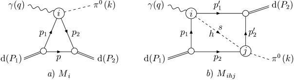
Figure 1: Feynman diagrams for the $\gamma d\!\to\!\pi^{0}d$ reaction. (a) single- and (b) double-scattering.

Figure 4: (a), (c), and (e) [(b), (d), and (f)] show real [image] parts of the loop integral $A_{11}$ of the double-scattering diagram (Fig.  1b) in “static” approximation with intermediate $\eta$ meson in reaction (1). The results are given for the values (a) and (b) $z\!=\!\cos\theta=\!0\,$; (c) and (d) $z=-0.55$; and (e) and (f) $z=-0.85$. Solid (dashed) curves correspond to the results with the Bonn (Gaussian) $s$ DWF.

Figure 5: The results for (a) and (b) Re$\,A_{11}$; (c) and (d) Im$\,A_{11}$; and (e) and (f) $|A_{11\,}|^{2}$ at (a), (c), and (e) $z\!=\!-0.55$; and (b), (d), and (f) $z\!=\!-0.85$ with the Gaussian $s$ DWF. Solid (dashed) curves correspond to “non-static” (“static”) case.

Figure 6: Differential cross sections of reaction (1) vs photon laboratory energy $E_{\gamma}$ at several values of $z\!=\!\cos\theta$. Dashed (dotted) and solid curves show the contributions of single (double) - scattering amplitudes and total amplitude, respectively. Dash-dotteded curves correspond to the contributions of total amplitude without $\omega$-exchange term. The results are obtained with energy-dependent total width of $N(1535)$. (a) $z=0$, (b) $z=-0.55$, (c) $z=-0.65$, (d) $z=-0.75$, (e) $z=-0.8$, and (f) $z=-0.85$,

Figure 7: The same as in Fig. 6 but the results are obtained with constant total width of $N(1535)$.

References

• (1) Y. Ilieva et al. [CLAS Collaboration], to be published in Nucl. Phys. A (2004) [nucl-ex/0309017].
• (2) R. L. Walker, Phys. Rev. 182, 1729 (1969).
• (3) R. G. Moorhouse, H. Oberlack, and A. H. Rosenfeld, Phys. Rev. D 9, 1 (1974).
• (4) H. Garcilazo and E. Moya de Guerra, Nucl. Phys. A562, 521 (1993).
• (5) D. Drechsel, O. Hanstein, S. S. Kamalov, and L. Tiator, Nucl. Phys. A645, 145 (1999) [nucl-th/9807001].
• (6) H. Garcilazo and E. Moya de Guerra, Phys. Rev. C 52, 49 (1995).
• (7) S. S. Kamalov, L. Tiator, and C. Bennhold, Phys. Rev. C 55, 98 (1997) [nucl-th/9602023].
• (8) G. Knöchlein, D. Drechsel, and L. Tiator, Z. Phys. A 352, 327 (1995) 327 [nucl-th/9506029].
• (9) M. Benmerrouche, N. C. Mukhopadhyay, and J. F. Zhang, Phys. Rev. D 51, 3227 (1995) [hep-ph/9412248].
• (10) F. Ritz and H. Arenhövel, Phys. Lett. B447, 15 (1999) [nucl-th/9810027];
Phys. Rev. C 64, 034005 (2001) [nucl-th/0011089].
• (11) C. Bennhold and H. Tanabe, Nucl. Phys. A530, 625 (1991).
• (12) L. A. Kondratyuk and F. M. Lev, Yad. Fiz. 23, 1056 (1976) [Phys. At. Nucl. (former Sov. J. Nucl. Phys.) 23, 556 (1976)];
Yad. Fiz. 27, 831 (1978) [Phys. At. Nucl. (former Sov. J. Nucl. Phys.) 27, 441 (1976)].
L. A. Kondratyuk, F. M. Lev, and L. V. Shevchenko, Yad. Fiz. 36, 377 (1982) [Phys. At. Nucl. (former Sov. J. Nucl. Phys.) 36, 220 (1982)].
• (13) B. M. Abramov et al., Nucl. Phys. A372, 301 (1981).
R. Keller et al., Phys. Rev. D 11, 2389 (1975).
M. Akemoto et al., Phys. Rev. Lett. 50, 400 (1983).
• (14) A. Imanishi et al., Phys. Rev. Lett. 54, 2497 (1985).
• (15) S. Eidelman et al. [Particle Data Group], Phys. Lett. B592, 1 (2004); http://pdg.lbl.gov.
• (16) R. A. Arndt, W. J. Briscoe, I. I. Strakovsky, and R. L. Workman, Phys. Rev. C 66, 055213 (2002) [nucl-th/0205067].
• (17) V. E. Tarasov, V. V. Baru, and A. E. Kudryavtsev, Yad. Fiz. 63, 871 (2000) [Phys. Atom. Nucl. 63, 801 (2000)].
• (18) R. Machleidt et al., Phys. Rep. 149, 1 (1987).
• (19) This “$c$-transformation” is applied to nucleon spin and isospin operators when writing the expression for the amplitude, we move along the nucleon lines (anticlockwise here) of the diagram in the direction of the nucleon momentum Tar .
• (20) R. A. Arndt, R. L. Workman, Z. Li, and L. D. Roper, Phys. Rev. C 42, 1864 (1990).
• (21) R. L. Crowford and W. T. Morton, Nucl. Phys. B211, 1 (1983).
• (22) R. Davidson, N. C. Mukhopadhyay, and R. Wittman, Phys. Rev. D 43, 71 (1991).
• (23) O. Dumbrajs et al., Nucl. Phys. B216, 277 (1983).
Refer to caption