Non-monotonic behavior of multiplicity fluctuations

Abstract

We discuss recently measured event-by-event multiplicity fluctuations in relativistic heavy-ion collisions. It is shown that the non-monotonic behavior of the multiplicity fluctuations as a function of collision centrality can be fully explained by the correlations between produced particles.

.

1 Introduction

Event-by-event fluctuations in heavy-ion collisions have been recently measured both at CERN SPS and BNL RHIC (see a brief review [1]). The data (usually used $F$ or $\Phi$ measures to quantify the fluctuations of transverse momentum) which show a non-trivial behavior as a function of collision centrality, have been theoretically discussed from very different points of view, including complete or partial equilibration, critical phenomena, string or cluster percolation, production of jets. In spite of these efforts a mechanism responsible for the fluctuations is far from being uniquely identified.

In [2] we have established connection of the $\Phi$-measure with the fluctuations of multiplicity and advocated that fluctuations of transverse momentum are practically irrelevant for the considered problem, i.e., for the apparent structure seen in collision centrality dependence. We argue [3] that the non-trivial behavior of the so called transverse momentum fluctuations (quantified by $F$ or $\Phi$ - measure) can be fully explained by the multiplicity fluctuations.

Recently, the NA49 Collaboration published very first data on multiplicity fluctuations as a function of collisions centrality [4], see also [5] in this volume. Unexpectedly, the ratio $Var(N)/\langle N\rangle$, where $Var(N)$ is the variance and $\langle N\rangle$ is the average multiplicity of negative particles, changes non-monotonically when number of wounded nucleons grows. It is close to unity at fully peripheral ($N_{w}\leq 10$) and completely central ($N_{w}\geq 250$) collisions but it manifests a prominent peak at $N_{w}\approx 70$. The measurement has been performed at the collision energy $158\,AGeV$ in the transverse momentum and pion rapidity intervals $(0.005,1.5)$ GeV and $(4.0,5.5)$, respectively. The azimuthal acceptance has been also limited, and about $20\%$ of all produced negative particles have been used in the analysis.

The aim of this paper is to show that the observed effect (non-monotonic dependence of the ratio $Var(N)/<N>$ on the number of projectile participants $N_{P}$, i.e., on the production volume $V$) stem from the correlations between produced particles and the correlations are of nuclear and electromagnetic interactions origin.

2 Correlations and fluctuations

Let us introduce the single-particle configuration distribution function [6]

$$n_{1}({\bf r}_{1})=n$$ (1)

where $n$ is (constant) density of particles. Two-particle configuration distribution function:

$$n^{\prime}_{2}({\bf r}_{1},{\bf r}_{2})=n^{2}\cdot n_{2}(|{\bf r}_{1}-{\bf r}_{2}|)\equiv n^{2}\cdot n_{2}(r)$$ (2)

is expressed by two-particle correlation function $\nu_{2}(r)$ following:

$$n_{2}(r)=1+\nu_{2}(r)$$ (3)

where, asymptotically for $r\rightarrow\infty$, $\nu_{2}(r)=0$ and $n_{2}(r)=1$.

For the volume $V$ one gets

$$<N_{V}>=\int\limits_{V}d{\bf r}_{1}n_{1}({\bf r}_{1})=\int\limits_{V}d{\bf r}_{1}n$$ (4)

$$<N_{V}^{2}>=\int\limits_{V}d{\bf r}_{1}n_{1}({\bf r}_{1})+\int\limits_{V}d{\bf r}_{1}\int\limits_{V}d{\bf r}_{2}n^{\prime}_{2}({\bf r}_{1},{\bf r}_{2})$$ (5)

The variance equals:

$$<N_{V}^{2}>-<N_{V}>^{2} = \int\limits_{V}d{\bf r}_{1}n_{1}({\bf r}_{1}){}$$ (6)

$${}+\int\limits_{V}d{\bf r}_{1}\int\limits_{V}d{\bf r}_{2}[n^{\prime}_{2}({\bf r}_{1},{\bf r}_{2})-n_{1}({\bf r}_{1})n_{1}({\bf r}_{2})]$$

and the normalized variance is given as:

$$\frac{<N_{V}^{2}>-<N_{V}>^{2}}{<N_{V}>}=1+\int\limits_{V}d{\bf r}\left[n\cdot n_{2}(r)-n\right]$$ (7)

Substituting now Eq. (3) to Eq. (7) one imediately leads to the formula:

$$\frac{<N^{2}>-<N>^{2}}{<N>}=1+n\int\limits_{V}d{\bf r}\nu_{2}(r)$$ (8)

which shows clearly that the normalized variance is given by two-particle correlation function.

Because:

$$\frac{Var(N)}{<N>}=1+nV<\nu_{2}>$$ (9)

where we note that the integral $\int\limits_{V}d{\bf r}_{1}\int\limits_{V}d{\bf r}_{2}\nu_{2}(|{\bf r}_{1}-{\bf r}_{2}|)=<\nu_{2}>V^{2}$, then it is clear that:

$$<\nu_{2}>=\frac{\left(\frac{Var(N)}{<N>}-1\right)}{<N>}$$ (10)

has numerical values close to zero. Determined this way $<\nu_{2}>$ do not depends on the detector acceptance $p$. Because, the normalized variance for the accepted particles:

$$\frac{Var(N)}{<N>}=(1-p)+p\cdot\frac{Var(N_{p=1})}{<N_{p=1}>}$$ (11)

and the accepted multiplicity:

$$<N>=p\cdot<N_{p=1}>$$ (12)

one finds from Eq. (10) the correlation function for the accepted particles $<\nu_{2}>=<\nu_{2}>_{p=1}$. Fig. 2 shows mean value of correlation function $<\nu_{2}>$ calculated from data on the ratio $Var\left(N\right)/<N>$ obtained at $158\,AGeV$ [4].

Figure 1: Mean value of correlation function calculated from data obtained at $158\,AGeV$.

Figure 2: The dependence of $\beta\cdot W\left(r\right)$ on relative distance $r$.

2.1 Simple example

Let the correlation function be in the form:

$$\nu_{2}({\bf r}_{1}-{\bf r}_{2})=\nu_{2}(r)=\exp(-2r/\lambda)$$ (13)

In this case:

$$\frac{Var\left(N\right)}{<N>} = 1+<N>\int\limits_{V}\int\limits_{V}d{\bf r}_{1}d{\bf r}_{2}\nu_{2}({\bf r}_{1}-{\bf r}_{2}){}$$ (14)

$$= 1+<N>\frac{2}{R^{2}}\int\limits_{0}^{R}(R-r)\nu_{2}(r)dr$$

and one gets

$$\frac{Var(N)}{<N>}=1+\frac{<N>}{2}\left(\frac{\lambda}{R}\right)^{2}\left(\exp\left(-2\frac{R}{\lambda}\right)-1+2\frac{R}{\lambda}\right)$$ (15)

It the limit $R>>\lambda$ we have

$$\frac{Var(N)}{<N>}\cong 1+<N>\frac{\lambda}{R}\cong 1$$ (16)

then for $R<<\lambda$

$$\frac{Var(N)}{<N>}\cong 1+<N>$$ (17)

3 Correlations and interactions

Two-particle distribution function $n^{\prime}_{2}(r)$ normalized for mean density, in the equilibrium case (with inverse temperature $\beta$) is given by the following Boltzmann factor [6]:

$$n^{-1}n^{\prime}_{2}(r)=n\cdot\exp\left(-\beta W(r)\right)$$ (18)

For the rigid spheres with the radius $d_{0}$, where

$$W(r)=\begin{array}[]{ll}\infty&r<2d_{0}\\ 0&r>2d_{0}\end{array}$$ (19)

we have the correlation function:

$$\begin{array}[]{ll}n_{2}(r)=0&r<2d_{0}\\ \nu_{2}(r)=-1&r<2d_{0}\end{array}$$ (20)

3.1 Two potentials

Let us consider two potentials: the electrostatic Debye potential [7]

$$\varphi_{e}(r)=e\frac{\exp\left(-r/\lambda_{e}\right)}{r}$$ (21)

and the nuclear Yukawa potential [8]:

$$\varphi_{n}(r)=-g\frac{\exp\left(-r/\lambda_{n}\right)}{r}$$ (22)

The attractive (nuclear) and repulsive (electrostatic) interactions leads to the effective energy:

$$W\left(r\right)=e\cdot\varphi_{e}\left(r\right)-g\cdot\varphi_{n}\left(r\right)$$ (23)

The dependence of $\beta\cdot W\left(r\right)$ on relative distance $r$ is presented in Fig. 2 for the numerical values: $\lambda_{n}=1.5\,fm]$ and $\lambda_{e}=3.5\,fm$.

For the radius $r>2d_{0}$ one can write the correlation function

$$\nu_{2}(r)=n_{2}(r)-1=\exp\left(a_{n}\frac{\exp\left(-r/\lambda_{n}\right)}{r}-a_{e}\frac{\exp\left(-r/\lambda_{e}\right)}{r}\right)-1$$ (24)

where strength factors are equal to: $a_{n}=\beta g^{2}$, $a_{e}=\beta e^{2}=\left(4\pi n\lambda_{e}^{2}\right)^{-1}$ and interaction lengths are: $\lambda_{n}=h\left(2\pi mc\right)^{-1}$, $\lambda_{e}=\left(4\pi e^{2}n\beta\right)^{-1/2}$.

In the first approximation one can write

$$\nu_{2}(r)\approx a_{n}\frac{\exp\left(-r/\lambda_{n}\right)}{r}-a_{e}\frac{\exp\left(-r/\lambda_{e}\right)}{r}$$ (25)

what allows for analytical integration $n\int d{\bf r}\nu_{2}(r)$ and analytical estimation of normalized variance $Var(N)/<N>$.

The problem of local and global fluctuations (the so called finite-size effect) was originally discussed by Nicolas [9] for correlation function:

$$\nu_{2}(r)=a\frac{\exp\left(-r/\lambda\right)}{r}$$ (26)

Integrating it (via the Fourier transformations method) in the spherical volume $V$ with the radius $R$ gives [10]:

$$f\left(R,\lambda,a\right) = \frac{Var(N)}{<N>}=1+n\int d{\bf r}a\frac{\exp\left(-r/\lambda\right)}{r}$$ (27)

$$= 1+6\pi an\frac{\lambda^{5}}{R^{3}}\Biggl{[}1-\left(\frac{R}{\lambda}\right)^{2}+\frac{2}{3}\left(\frac{R}{\lambda}\right)^{3}-\exp\left(-2R/\lambda\right)\cdot\left(1+\frac{R}{\lambda}\right)^{2}\Biggr{]}$$

Asymptotically for small $R$ $(V=4/3\pi R^{3}<<\lambda^{3})$ one gets:

$$f\left(R,\lambda,a\right)=\frac{Var(N)}{<N>}\propto 1+\frac{8\pi anR^{2}}{5}$$ (28)

whereas for large $R$ $(V=4/3\pi R^{3}>>\lambda^{3})$ one gets:

$$f\left(R,\lambda,a\right)=\frac{Var(N)}{<N>}\propto 4\pi an\lambda^{2}\left(1-\frac{3}{2}\frac{\lambda}{R}\right)$$ (29)

For our correlation function $\nu_{2}\left(r\right)$, given by Eq. (25), one immediately gets:

$$\frac{Var\left(N\right)}{<N>}=f\left(R,\lambda_{n},a_{n}\right)-f\left(R,\lambda_{e},a_{e}\right)$$ (30)

In this paper the integral Eq. (8) has been calculated via Monte-Carlo method, assuming the homogenous spherical production volume, $V\sim N_{P}$, to be proportional to the number of participants $N_{P}$. Fig.4 shows normalized variance of the multiplicity distribution and mean multiplicity of negatively charged particles produced in collisions at $158\,AGeV$ fitted by the two potentials model. It is interesting to note that different shapes of the production region (with particle density distribution $n\left(r\right)$) influence the presented results for the large number of participants $N_{P}$ and allow us to obtain much more satisfactory fit to experimental data.

3.2 Single potential (dipole-dipole interactions)

Electrostatic correlations play an important role in analysis of thermodynamic system [11, 12]. In following, we analyze one more (speculative, but possible) scenario, which result in non-monotonic behavior of fluctuations.

Let us assume that the particles are produced in pairs $\left(\pi^{+}\pi^{-}\right)$ creating dipoles. The potential describing interaction between ${\bf p}_{1}$ and ${\bf p}_{2}$ dipoles is given by:

$$\varphi(r) = \frac{1}{r^{3}}\Biggl{(}{\bf p}_{1}{\bf p}_{2}-\frac{3\left({\bf p}_{1}{\bf r}\right)\left({\bf p}_{2}{\bf r}\right)}{r^{2}}\Biggr{)}$$ (31)

$$= \frac{<p>^{2}}{r^{3}}\left(\sin\theta_{1}\sin\theta_{2}\cos\left(\phi_{1}-\phi_{2}\right)+\cos\theta_{1}\cos\theta_{2}-3\cos\theta_{1}\cos\theta_{2}\right)$$

$$= \frac{<p>^{2}}{r^{3}}f\left(\theta,\phi\right)$$

and changes from $-2<p>^{2}/r^{3}$ to $+2<p>^{2}/r^{3}$, depending on dipoles space arrangement. Changing the polarization of dipoles depending on distance between them $f\left(\theta,\phi\right)\rightarrow f\left(r,\theta,\phi\right)$ allows for transition from negative values of potential (low values of $r$; particles correlation) to positive (big $r$; particles anti-correlation). For instance the dependence of the type:

$$f\left(r,\theta,\phi\right)=-2\exp\biggl{[}-\left(r/\lambda\right)^{3}\biggr{]}+2\biggl{(}1-\exp\biggl{[}-\left(r/\lambda\right)^{3}\biggr{]}\biggr{)}$$ (32)

provides to the correlation function $\nu_{2}(r)$ which allow for approximate description of experimental data (c.f. Fig.4, where we fit data with the parameter $\lambda=2.6\,fm$). One can get the effect of changing $f\left(r,\theta,\phi\right)$ via correlation between the dipole angles, for example:

$$\Delta\theta=\pi\biggl{(}1-\exp\biggl{[}-\left(r/\lambda\right)^{3}\biggr{]}\biggr{)}$$ (33)

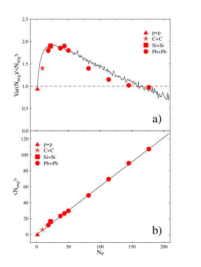
Figure 3: Normalized variance of the multiplicity distribution (a) and mean multiplicity (b) of negatively charged particles produced in collisions at $158\,AGeV$ [4] fitted by the two potentials model.

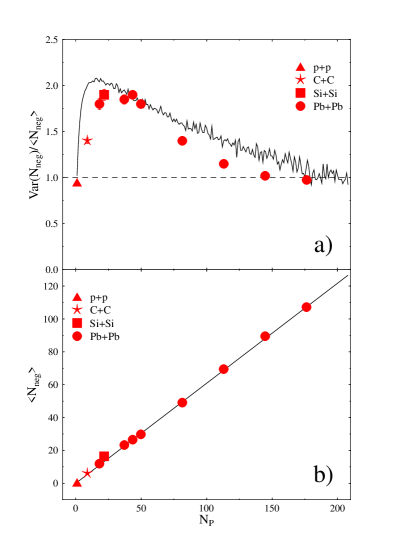
Figure 4: Normalized variance of the multiplicity distribution (a) and mean multiplicity (b) of negatively charged particles produced in collisions at $158\,AGeV$ [4] fitted by the dipole model.

4 Connections to percolation

The particles situated in correlation length $\lambda$ distance each other builds the cluster. For low $R<\lambda/2$ the whole production volume belongs to the single cluster. If the size of the fireball increases ”the percolation” to the next clusters appear [13]. The number of percolation clusters $M_{C}$ is proportional to:

$$M_{C}\sim\left(\frac{2R}{\lambda}\right)^{3}$$ (34)

The number of particle pairs in distance $d$, included in the sphere with radius $R$ is distributed as:

$$P(d)=\begin{array}[]{ll}\frac{d}{R}&0<d<R\\ 2-\frac{d}{R}&R<d<2R\end{array}$$ (35)

and the number of particles pairs with relative distance $d<\lambda$ to the total number of pairs is given by:

$$M_{P}=\frac{M_{P}\left(<\lambda\right)}{M_{TOT}}=\begin{array}[]{ll}2\left(\frac{\lambda}{2R}\right)^{2}&R>\lambda\\ 4\left(\frac{\lambda}{2R}\right)-2\left(\frac{\lambda}{2R}\right)^{2}-1&\frac{\lambda}{2}<R<\lambda\\ 1&R<\frac{\lambda}{2}\end{array}$$ (36)

In the simplest approximation the number of particle pairs for single cluster equals $M_{P}/M_{C}$ and correlation function $\nu_{2}\sim\left(M_{P}/M_{C}\right)^{2}$ is given by:

$$\nu_{2}=\begin{array}[]{ll}\Bigl{(}2\left(\frac{\lambda}{2R}\right)^{5}\Bigr{)}^{2}&R>\lambda\\ \Biggl{(}\left(\frac{\lambda}{2R}\right)^{3}\biggl{[}4\left(\frac{\lambda}{2R}\right)-2\left(\frac{\lambda}{2R}\right)^{2}-1\biggr{]}\Biggr{)}^{2}&\frac{\lambda}{2}<R<\lambda\\ 1&R<\frac{\lambda}{2}\end{array}$$ (37)

5 Connections to nonextensivity

Let us now continue discussion of the multiplicity fluctuations from the point of view of its possible connection with nonextensivity (for other hints on nonextensivity in hadronic production processes and references to nonextensive statistics, see [14, 15]). When there are only statistical fluctuations in the hadronizing system one should expect the Poissonian form of the multiplicity distribution. The existence of intrinsic (dynamical) fluctuations result in broader distributions usually expressed via Negative Binomial form and characterized by the parameter (so called the inverse number of ”clans”):

$$k^{-1}=\frac{Var(N)}{<N>^{2}}-\frac{1}{<N>}.$$ (38)

By using Eq. (9), $Var\left(N\right)/<N>=1+<N><\nu_{2}>$, then one gets:

$$q-1=k^{-1}=<\nu_{2}>$$ (39)

where $q$ is an nonextensivity parameter.

Small systems (with diameters non exceeding correlation length) are characterized by the parameter $q>1$ and just in the thermodynamic limit $q=1$ (for big size systems with $R>>\lambda$, where the correlation effects are small and all subsystems are characterized by the same temperature).

The $q$ parameter could be connected with the number of correlation clusters (”copies” of the system) $M_{C}$. If $M_{C}$ grows, the Tsallis entropy [16]:

$$S=\lim_{q\to 1}\frac{\sum p^{q}-1}{1-q}$$ (40)

where nonextensivity parameter $q=1+m\sim 1+\frac{1}{M_{C}}$ leads to the thermodynamic Shannon entropy:

$$S=-\sum p\ln p$$ (41)

because:

$$\ln p=\lim_{m\to 0}\frac{p^{m}-1}{m}.$$ (42)

Experimental data prefers dependence of the type:

$$M_{C}\sim\exp\Biggl{(}\left(\frac{R}{\lambda}\right)^{3}\Biggr{)}.$$ (43)

6 Conclusions

The observed effect (non-monotonic dependence of the ratio $Var(N)/<N>$ on production volume $V\sim N_{P}$) stem from the correlations between produced particles. The correlations are of nuclear and electromagnetic interactions origin. It is possible to describe the appearance of a prominent peak in $Var(N)/<N>$ at number of participants $N_{P}\approx 35$, for charged particles. For the neutral particles we observe lack of non-monotonic behavior of $Var(N)/<N>$ when number of wounded nucleons grows (satisfy the experimental observation [17]). Effect depends on energy, because particles density $n$ changes with energy (the magnitude of the effect $\simeq n$ and position of maximum also shifts, because correlation length $\lambda_{e}\simeq 1/\sqrt{n}$).

References

References

• [1] Mitchell J T, Preprint nucl-ex/0404005
• [2] Rybczyński M, Włodarczyk Z, Wilk G, 2004, Acta Phys. Pol. B 35 819
• [3] Mrówczyński S, Rybczyński M, and Włodarczyk Z, Preprint nucl-th/0407012
• [4] Gaździcki M et al. (NA49 Collaboration), 2004 J. Phys. G 30 S701
• [5] Rybczyński M et al. (NA49 Collaboration), 2004, Multiplicity fluctuations in relativistic heavy ion collisions (this proceedings)
• [6] Balescu R 1975 Equilibrium and Nonequilibrium Statistical Mechanics (New York: Wiley Interscience)
• [7] Debye P, Hückel E, 1923, Phys. Zs. 24 185
• [8] Yukawa H, 1935, Proc. Phys. Math. Soc. Jap. 17 48
• [9] Nicolas G, 1972, J. Stat. Phys. 6 195
• [10] Gardiner C W 1986 Handbook of Stochastic Methods for Physics, Chemistry and the Natural Science (Berlin: Springer)
• [11] Brown L S, Yaffe L G, 2001, Phys. Rep. 340 1
• [12] Levin Y, 2002, Rep. Prog. Phys. 65 1577
• [13] Stauffer D, Aharony A 1994 Introduction to Percolation Theory (Taylor & Francis)
• [14] Wilk G, Włodarczyk Z, 2000, Phys. Rev. Lett. 84 2770
• [15] Navarra F S, Utyuzh O V, Wilk G, Włodarczyk Z, 2003, Phys. Rev. D 67 114002; 2004, Physica A 340 467
• [16] Tsallis C A, 1988, J. Stat. Phys. 52 479 (a periodically updated bibliography can be found at: http://tsallis.cat.cbpf.br/biblio.htm)
• [17] Aggarwal M M et al. (WA98 Collaboration), 2002 Phys. Rev C 65 054912