Probing the nuclear energy functional at band termination

Abstract

A systematic study of terminating states in $A$$\sim$50 mass region using the self-consistent Skyrme-Hartree-Fock model is presented. The objective is to demonstrate that the terminating states, due to their intrinsic simplicity, offer unique and so far unexplored opportunities to study different aspects of the effective NN interaction or nuclear local energy density functional. In particular, we demonstrate that the agreement of the calculations to the data depend on the spin fields and the spin-orbit term which, in turn, allows to constrain the appropriate Landau parameters and the strength of the spin-orbit potential.

I Introduction

Within the mean-field approach the spin-orbit ($\ell s$) splitting is usually studied via the comparison of theoretical and experimental single-particle ($sp$) energies of the $\ell s$-doublet. The requirement is that both $\ell s$-partners should be simultaneously occupied [Rut98] ; [Lop00] . The method assumes that under such conditions the core polarization effects, which are known to modify strongly sp energies [Ham76] ; [Ber80] , are similar for $\ell s$-partners and therefore do not affect the $\ell s$-splittings, at least not in a major way.

The method requires by definition precise empirical knowledge on $sp$ energies of deep-hole states which are very difficult to measure. In addition, particle vibration coupling may contribute to the splitting and perturb the pure $sp$ picture. The available data on $\ell s$-splittings and their isotopic or isotonic dependence are therefore both scarce and uncertain. For example, in the $A$$\sim$40 mass region, which is of primary interest in this work, the most recent evaluations [Oro96] give $\Delta\varepsilon_{d_{3/2}-d_{5/2}}$$\approx$ 6 MeV in ⁴⁰Ca and $\Delta\varepsilon_{d_{3/2}-d_{5/2}}$$\approx$ 5 MeV in ⁴⁸Ca, respectively, while older works give $\Delta\varepsilon_{d_{3/2}-d_{5/2}}$$\approx$ 6.8 MeV [Swi66] , $\approx$ 7.3 MeV [Tyr66] , and $\approx$ 7.7 MeV [Ray79] in ⁴⁰Ca and $\approx$ 5.3 MeV [Ray79] in ⁴⁸Ca. More detailed information on $sp$ levels can be found in Ref. [Isa02] .

In this work we want to pursue a novel method to study the $\ell s$-potential by exploring high-spin data. The method is based on a direct comparison of the excitation energies of terminating states [which are maximum-spin states within a given $sp$ configuration] for two carefully selected configurations. In this study we limit ourselves to the $d_{3/2}^{-1}f_{7/2}^{n+1}$ and $f_{7/2}^{n}$ configurations in $A$$\sim$50, 20$\leqslant$Z$<$N$\leqslant$24 nuclei, where $n$ denotes the number of valence particles outside the ⁴⁰Ca core. The difference, $\Delta E$, between the excitation energies of states terminating within the $d_{3/2}^{-1}f_{7/2}^{n+1}$ and $f_{7/2}^{n}$ configurations is dominated by the size of the magic gap 20. The magnitude of the magic gap 20 is in turn governed by the strength of the $\ell s$-potential. Indeed, for the spherical Nilsson Hamiltonian [Nil55] , i.e. the three-dimensional harmonic-oscillator (HO) potential augmented by a one-body spin-orbit $-2\kappa\hbar\omega_{o}{\bm{\ell}}{\bm{s}}$ and orbit-orbit $-\kappa\mu\hbar\omega_{o}{\bm{\ell}}^{\,2}$ term one has:

$$\hat{H}_{Nilsson}-\frac{3}{2}\hbar\omega_{o}=\hbar\omega_{o}\left\{N-\kappa\left[2{\bm{\ell}}{\bm{s}}+\mu({\bm{\ell}}^{\,2}-\langle{\bm{\ell}}^{\,2}\rangle_{N})\right]\right\}.$$ (1)

Hence, within the Nilsson model, which is considered to be a fundamental approximation for the nuclear mean-field potential, the magnitude of the magic gap 20, or more precisely the $f_{7/2}$$-$$d_{3/2}$ splitting reads:

$$\Delta e_{20}=\hbar\omega_{o}(1-6\kappa-2\kappa\mu).$$ (2)

In light nuclei the nuclear potential resembles the pure HO, thus $\mu\sim 0$. Hence, within the Nilsson model, the $\ell s$-term plays a dominant role in establishing the size of the magic gap 20. Indeed, $\hbar\omega_{o}$ determines the global energy scale in low energy nuclear physics and one does not expect this value to change substantially. Although Eq. (2) pertains to the $f_{7/2}$$-$$d_{3/2}$ splitting, the conclusion drawn above seems to be easily extendable to heavier nuclei since there $\mu$$\rightarrow$1/2 as a consequence of approximate pseudo-SU(3) symmetry [Boh82] ; [Bah92] ; [Gin97] .

By limiting ourselves to the study of band terminating states only, we access the regime of essentially unperturbed $sp$ motion, where correlations going beyond mean-field are expected to be strongly suppressed. Indeed, the success of simple Nilsson-Strutinsky calculations of terminating bands by Ragnarsson and coworkers, for review see [Afa99] , nicely confirm the structural purity and $sp$ nature of the terminating states. However, within the self-consistent approaches, in particular within the Skyrme-Hartree-Fock (shf) approach which is used here, there are additional difficulties and in turn uncertainties related to the limited knowledge of the time-odd components of the mean-field. Direct studies of these terms are not only scarce but also in many cases inconclusive, see [Sat04] and refs. quoted therein. In contrast, the structural simplicity of terminating states is appealing and allows for a direct study of these terms.

The method proposed here to determine the $\ell s$-term has clear advantages over the standard method mentioned at the beginning: (i) it uses terminating states which are probably the best examples of unperturbed single-particle motion; (ii) the terminating states are uniquely defined implying that configuration mixing going beyond mean-field is expected to be marginal; (iii) shape polarization is included automatically within the calculations scheme and no further ad hoc assumptions are necessary; (iv) a wide set of rather precise experimental data is already available throughout the periodic table.

The paper is organized as follows. Sect. II overviews available empirical data. Sect. III briefly recalls the local energy density functional (ledf) formulation of the shf method. Sect. IV reveals the problems related to spin fields emerging from the Skyrme force induced local energy density functional (s-ledf) in $N$$\sim$$Z$ nuclei both in the ground state as well as at the band termination. It is shown, that an unification of spin fields cures these problems leading to an unified description of terminating states. The remaining discrepancy between experiment and theory can further be reduced by tuning (weakening) the strength of the spin-orbit interaction as shown in Sect. V. Finally, in Sect. VI we test the additivity relation for the only known case of a $2p$-$2h$ excitation across the magic gap in ⁴⁵Sc. All shf calculations presented in this paper were done using the shf code hfodd of Dobaczewski, Dudek, and Olbratowski [Dob00] ; [Dob04] .

II Experimental data

	Ref.	$\quad\quad f_{7/2}^{n}:$	$E[I_{max}]$	$I_{max}$	$\quad\quad d_{3/2}^{-1}f_{7/2}^{n+1}:$	$E[I_{max}]$	$I_{max}$	$\quad\quad\quad\Delta E_{exp}$
${}^{42}_{20}\mbox{Ca}_{22}$	[Lac03]		3.189	6+		8.297	11-	5.108
${}^{44}_{20}\mbox{Ca}_{24}$	[Lenzi]		10.568	8+		5.088	13-	5.480
${}^{44}_{21}\mbox{Sc}_{23}$	[Lac03a]		9.141	11+		3.567	15-	5.574
${}^{45}_{21}\mbox{Sc}_{24}$	[Bed01]		5.417	23/2-		11.022	31/2+	5.605
	[Lenzi]					15.701	35/2-	10.284
${}^{45}_{22}\mbox{Ti}_{23}$	[Lenzi]		7.143	27/2-		13.028	33/2+	5.885
${}^{46}_{22}\mbox{Ti}_{24}$	[Lenzi]		10.034	14+		15.549	17-	5.515
${}^{47}_{23}\mbox{V}_{24}$	[Bra01]		10.004	31/2-		15.259	35/2+	5.255

Table 1: Spins and excitation energies of terminating states in $20\leqslant Z<N\leqslant 24$ nuclei. The first two columns are representative the for $f_{7/2}^{n}$ configuration where $n$ denotes the number of valence particles outside the ⁴⁰Ca core. The next two columns are representative for the $d_{3/2}^{-1}f_{7/2}^{n+1}$ configuration involving the $1p$-$1h$ proton excitation across the magic gap 20. For the case of ⁴⁵Sc, data on the $d_{3/2}^{-2}f_{7/2}^{n+2}$ configuration involving two $1p$-$1h$ excitations from the $d_{3/2}$ to $f_{7/2}$ are also included. The relative excitation energies between the two configurations are given in the last column.

All available experimental data on the terminating states for $f_{7/2}^{n}$ and $d_{3/2}^{-1}f_{7/2}^{n+1}$ configurations in $A$$\sim$50, 20$\leqslant$Z$<$N$\leqslant$24 nuclei where both states are known are listed in Tab. 1. In the present data set we have excluded the $N$=$Z$ nuclei since in these nuclei the terminating state $d_{3/2}^{-1}f_{7/2}^{n+1}$ is not uniquely defined. Indeed, two states with the same value of $I_{max}$ can be formed, having approximately (due to the weak isospin symmetry breaking) symmetric ($T=0$) and antisymmetric ($T=1$) proton-neutron configurations, respectively. $N$=$Z$ nuclei will be addressed in a forthcoming paper [Sat04b] .

The differences in excitation energies, $\Delta E_{exp}$, listed in the last column of Tab. 1 are fairly constant. The mean value equals $\overline{\Delta E_{exp}}=5.489$ MeV while the standard deviation is $\sigma=0.251$ MeV i.e. at the level of $\sim$ 5% only. This suggests that the bulk part of $\Delta E_{exp}$ is indeed related to the energy of $1p$-$1h$ excitation across the gap 20, and that polarization effects are either weak or, most likely, cancel out.

This conclusion is further supported by a recent measurement in ⁴⁵Sc of a terminating state at spin $I^{\pi}_{max}=35/2^{-}$ and excitation energy of 15.701 MeV [Lenzi] . This state involves the $2p$-$2h$ excitation from the $\pi d_{3/2}$ to $\pi f_{7/2}$ sub-shell. The excitation energy with respect to the aligned $f_{7/2}^{n}$ state equals $\Delta E_{2p2h}=10.284$ MeV. For the extreme case of pure additivity this excitation can be composed from two, uniquely defined, $1p$-$1h$ states terminating at $I^{\pi}_{max}=29/2^{+}$ (termination at unfavored signature) which both are known. The empirical excitation energies of these states, relative to the aligned $f_{7/2}^{n}$ state, are 4.753 MeV and 5.783 MeV, respectively. The resulting sum yields $\Delta E^{(add)}_{2p2h}$=10.536 MeV implying that additivity holds within $\sim$2%.

III Skyrme-Hartree-Fock local energy density functional

The starting point of the shf approach is an energy density functional which, in the isoscalar-isovector $t=0,1$ representation, takes the following form:

$${\cal E}^{Skyrme}=\sum_{t=0,1}\int d^{3}{\bm{r}}\left[{\mathcal{H}}_{t}^{(TE)}({\bm{r}})+{\mathcal{H}}_{t}^{(TO)}({\bm{r}})\right].$$ (3)

The local energy density functional ${\mathcal{H}}$ (ledf) is uniquely expressed as a bilinear form of time-even (te) $\rho,\tau,\overleftrightarrow{J}$ and time-odd (to) $\bm{s},\bm{T},\bm{j}$ local densities, currents, and by their derivatives:

$${\mathcal{H}}_{t}^{(TE)}({\bm{r}})=C_{t}^{\rho}\rho_{t}^{2}+C_{t}^{\Delta\rho}\rho_{t}\Delta\rho_{t}+C_{t}^{\tau}\rho_{t}\tau_{t}+C_{t}^{J}\overleftrightarrow{J}_{t}^{2}+C_{t}^{\nabla J}\rho_{t}{\bm{\nabla}}\cdot{\bm{J}}_{t},$$ (4)

$${\mathcal{H}}_{t}^{(TO)}({\bm{r}})=C_{t}^{s}\bm{s}_{t}^{2}+C_{t}^{\Delta s}\bm{s}_{t}\Delta\bm{s}_{t}+C_{t}^{T}\bm{s}_{t}\cdot\bm{T}_{t}+C_{t}^{j}{\bm{j}}_{t}^{2}+C_{t}^{\nabla j}\bm{s}_{t}\cdot({\bm{\nabla}}\times{\bm{j}}_{t}).$$ (5)

The division of ledf into te and to parts is very convenient since the latter contributes only when time reversal symmetry is broken.

In the above formulas $\overleftrightarrow{J}_{t}^{2}\equiv\sum_{\mu\nu}J_{\mu\nu,t}^{2}$ while the vector spin-orbit density, ${\bm{J}}_{t}$, is not an independent quantity but constitutes an antisymmetric part of the tensor density, i.e., ${\bm{J}}_{t}\equiv\sum_{\mu\nu}\epsilon_{\mu\nu}J_{\mu\nu,t}$. Definitions of all local densities and currents $\rho,\tau,\overleftrightarrow{J},\bm{s},\bm{T},\bm{j}$ can be found in numerous references and will not be repeated here. We follow the notation used in Refs. [Dob95] ; [Dob00] ; [Ben02] where references to earlier works can be found as well.

By taking an expectation value of the Skyrme force over the Slater determinant one obtains ledf (3)–(5) with 20 coupling constants $C$ that are expressed uniquely through the 10 parameters $x_{i},t_{i},\,i=0,1,2,3$ and $W,\alpha$ of the standard Skyrme force. The appropriate formulas can be found, e.g., in Refs. [Dob95] ; [Ben02] . Due to the local gauge invariance (which includes the Galilean invariance) of the Skyrme force [Eng75] ; [Dob95] only 14 coupling constants $C$ are independent quantities. The local gauge invariance links three pairs of time-even and time-odd constants in the following way:

$$C_{t}^{j}=-C_{t}^{\tau},\quad C_{t}^{J}=-C_{t}^{T}\quad C_{t}^{\nabla j}=C_{t}^{\nabla J}.$$ (6)

Since the shf approach uses interaction-induced coupling constants $C$ it constitutes a restricted version of the local energy density theory of Hohenberg-Kohn-Sham [Hoh64] ; [Koh65] ; [Koh98] type. However, only very few shf approaches rigidly enforce the Skyrme-force-related values of $C$. Among those studied here these include SkP [Dob84] , SkXc [Bro98] , and Sly5 [Cha97] . Other forces studied here, including Sly4 [Cha97] , SIII [Bei75] , SkO [Rei99] , and SkM^⋆ [Bar82] disregard the tensor terms by setting $C_{t}^{J}=C_{t}^{T}\equiv 0$. This is not only due to practical reasons (these terms are the most difficult technically) but also due to lack of clear experimental information that would allow for reasonable estimates of their strengths. Moreover, in the case of SkO we were forced to set $C_{t}^{\Delta s}\equiv 0$ to assure convergence. All versions of ledf that use the Skyrme-force-induced $C$ values, including those taking $C_{t}^{J}=C_{t}^{T}\equiv 0$ will be called later Skyrme-ledf (s-ledf).

IV The spin fields

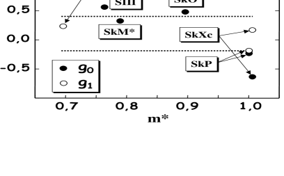
Figure 1: Isoscalar Landau parameters $g_{0}$ (solid circles) and $g_{1}$ (open circles) for various Skyrme forces. Vertical lines marks the values $g_{0}$=0.4 and $g_{1}$=–0.19 recommended by Bender et al. [Ben02] from their study of the Gamow-Teller resonances.

The strengths of the spin fields, $C^{s}_{t}{\bm{s}}^{2}$ and $C^{\Delta s}_{t}{\bm{s}}$$\cdot$$\Delta{\bm{s}}$, emerging from the Skyrme force appear to be more or less accidental. This is illustrated in Fig. 1 showing the isoscalar Landau parameters $g_{0}$ and $g_{1}$ calculated for the Skyrme forces under study. The Landau parameters are related to the ledf strengths in the following way [Ben02] :

$$g_{0}=N_{0}(2C_{0}^{s}+2C_{0}^{T}\beta\rho_{0}^{2/3}),\quad\quad g_{1}=-2N_{0}C_{0}^{T}\beta\rho_{0}^{2/3},$$ (7)

$$g_{0}^{\,\prime}=N_{0}(2C_{1}^{s}+2C_{1}^{T}\beta\rho_{0}^{2/3}),\quad\quad g_{1}^{\,\prime}=-2N_{0}C_{1}^{T}\beta\rho_{0}^{2/3},$$ (8)

where $\beta=(3\pi^{2}/2)^{2/3}$, and $N_{0}^{-1}=\pi^{2}\hbar^{2}/2m^{\star}k_{F}$ is an effective-mass-dependent normalization factor. The Skyrme-force-induced $g_{0}$ and $g_{1}$ parameters, see Fig. 1, are indeed scattered rather randomly reflecting the fact that Skyrme forces are fitted ultimately to the te channel while the to components of the s-ledf are only cross-checked mostly through the high-spin (cranking) applications. In Ref. [Ben02] the preferred values $g_{0}$=0.4, $g_{0}^{\,\prime}$=1.2 and $g_{1}$=–0.19, $g_{1}^{\,\prime}$=0.62 have been established from the analysis of the Gamow-Teller resonances, see also Ref. [Ost92] and refs. quoted therein. These values were obtained under an additional assumption of the density independence of $C_{t}^{s}$ and for $C_{t}^{\Delta s}$$\equiv$0. The ledf with spin fields defined in this way will be called later the Landau-ledf (l-ledf).

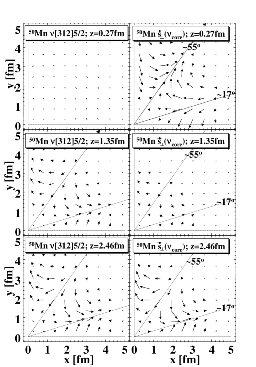
Figure 2: The $\vec{\bm{s}}_{\perp}$ component of the spin density (in arbitrary units) in the ground state of ⁵⁰Mn, calculated for three selected cross sections at $z$=0.27 fm (upper part) $z$=1.35 fm (middle part), and $z$=2.46 fm (lower part). Left panels show the contribution of the odd neutron right panels show polarization effect exerted by the odd neutron on the neutron core. For this case $\vec{\bm{s}}_{\perp}^{\,\nu}\approx\vec{\bm{s}}_{\perp}^{\,\pi}$, see text for further detail.

IV.1 The spin fields at the ground state

Before proceeding to the study of the terminating states let us discuss the spin fields of the ground states (calculated in HF approximation) of $N$$\approx$$Z$ nuclei. It is known that the binding energies calculated using the complete s-ledf functional exhibit a rather peculiar behavior in odd-odd $T_{z}=0$ and some odd-$A$ $|T_{z}|=1/2$ nuclei [Sat99] . It manifests itself via additional binding energy of the order of $\sim 1$ MeV as compared to the shf calculations using only the te part of the s-ledf. The effect disappears for $|T_{z}|>1$ nuclei.

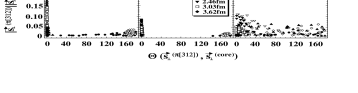
Figure 3: Product of $|\vec{s}^{\,\pi[512]}_{\perp}({\bm{r}})||\vec{s}^{\,core}_{\perp}({\bm{r}})|$ reflecting the magnitude of the spin fields (in arbitrary units) versus the classical angle between these vectors $\theta$, corresponding to their relative orientation. a) $N$=$Z$ o-o nucleus ⁵⁰Mn, b) $N-Z=1$ odd-$A$ nucleus ⁵¹Mn, c) $N-Z=2$ o-o nucleus ⁵²Mn. All points calculated at a fix value of the $z$ coordinate and different values of the ($x$,$y$) coordinates are labeled by the same symbol, as indicated in the legend.

The enhancement in the binding energy of $N$$\approx$$Z$ nuclei is due to a strong polarization effect exerted by the spin field of the odd-particle(s) on the spin field of the core, as illustrated in Figs. 2 and 3 for a representative example of the manganese isotopes. Fig. 2 shows the $Oxy$ component of the spin density $\vec{\bm{s}}_{\perp}$ in ⁵⁰Mn for three selected cross sections through this axially deformed nucleus, that include the near-equatorial plane at $z$=0.27 fm as well as $z$=1.35 fm and 2.46 fm planes. To visualize the polarization effect we decompose the spin density into contributions of the valence particles (note that $\vec{\bm{s}}^{\pi}\approx\vec{\bm{s}}^{\nu}$ in this $N$=$Z$ nucleus) and the core. The topology of the surfaces shown on the left hand side reflects the structure of the dominant asymptotic [312]5/2 Nilsson component in the wave function of the valence particle. Indeed, the one particle contribution to the spin field in a simplex-conserving axial HO basis state:

$$\Psi_{Nn_{z}|\Lambda|;s=\pm i}=\frac{1}{\sqrt{2}}(\Psi_{Nn_{z}\Lambda;1/2}\pm i\Psi_{Nn_{z}-\Lambda;-1/2})\quad\mbox{where}\quad\Psi_{Nn_{z}\Lambda}=\psi_{Nn_{z}|\Lambda|}e^{i\Lambda\varphi},$$ (9)

is

$$s_{x}=-\frac{1}{2}|\psi_{Nn_{z}|\Lambda|}(\rho,z)|^{2}\sin 2\Lambda\varphi,\quad s_{y}=-\frac{1}{2}|\psi_{Nn_{z}|\Lambda|}(\rho,z)|^{2}\cos 2\Lambda\varphi,\quad s_{z}=0,$$ (10)

see Ref. [Dob00] for further details. Hence, $|s_{x}|/|s_{y}|=|\mbox{ctg}2\Lambda\varphi|$ and the plot of $\vec{\bm{s}}_{\perp}$ shows the characteristic ”vortex” lines for $|s_{x}|/|s_{y}|=1$, i.e., for $\varphi=[45^{\circ}+n\pi]/2\Lambda$ where $n=0,1,2,...$. Two such lines that appear in Fig. 2 are consistent with $\Lambda=2$. Moreover, the small values of $s_{xy}\sim 0$ over the entire equatorial plane at $z=0.27$ fm are due to $\psi_{[312]}\sim H_{1}(z\approx 0)\approx 0$. Calculations also show that although $s_{z}\neq 0$ the condition $|s_{z}|\ll|s_{\perp}|$ is well fulfilled for most cases.

Correlation between the spin field $\vec{\bm{s}}^{\,\pi[512]}_{\perp}({\bm{r}})$ due to the occupation of the [512]5/2 orbital by the valence proton and that of the core $\vec{\bm{s}}^{\,core}_{\perp}({\bm{r}})$ (polarization effect) is illustrated in Fig. 3. The figure shows the product $|\vec{\bm{s}}^{\,\pi[512]}_{\perp}({\bm{r}})|\cdot|\vec{\bm{s}}^{\,core}_{\perp}({\bm{r}})|$ that reflects the magnitude of the spin fields versus the classical angle between these vectors $\theta$ that reflects their relative orientation. The figure clearly illustrates that in an o-o $N$=$Z$ nucleus the core polarization is strongest and of almost purely ferromagnetic type. In an odd-A $N$$-$$Z$=$\pm$1 nuclei the effect is quenched but remains to be of ferromagnetic type. Hence, the role of the spin fields in these nuclei is maximal. In $|N-Z|>1$ nuclei the induced (core) spin field appears to be quenched even further and, additionally, not coherent with the valence-particle(s) spin field, particularly in o-o nuclei, as depicted in Fig. 3c.

At least two very important conclusions can be drawn from this analysis. (i) The coherence of the spin fields in $N$$\sim$$Z$ nuclei may cause a strong polarization of the nucleus. (ii) The magnitude of the spin-field-induced effects is predicted to depend strongly on isospin. These two observations give an unique opportunity to resolve the strength of the spin fields, in particular, by using high spin states where spin fields are expected to be enhanced.

IV.2 The spin fields at the band termination

Fig. 4a shows the calculated energy differences for the terminating states $\Delta E_{th}=E_{th}[d_{3/2}^{-1}f_{7/2}^{n+1}]-E_{th}[f_{7/2}^{n}]$ relative to the experimental data $\Delta E_{exp}$ given in Tab. 1, i.e. the values of $\Delta E\equiv\Delta E_{exp}-\Delta E_{th}$. The first striking observation stemming from this calculation is that all considered Skyrme forces systematically underestimate empirical data by at least 10% . In case of the SkM^∗ and SkP parameterizations the difference even exceeds 20$\div$30%. The disagreement is unexpectedly large provided the structural simplicity of the terminating states.

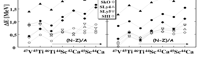
Figure 4: Calculated energy differences for the terminating states $\Delta E_{th}=E_{th}[d_{3/2}^{-1}f_{7/2}^{n+1}]-E_{th}[f_{7/2}^{n}]$ relative to the experimental data $\Delta E\equiv\Delta E_{exp}-\Delta E_{th}$ where $\Delta E_{exp}$ are listed in Tab. 1. The left panel shows shf calculations while right part illustrates calculations using l-ledf.

Let us further observe that the values of $\Delta E$ calculated using SLy4 and SLy5 forces, which are in general rather similar to $\Delta E$ obtained using SIII or SkO forces, increase rapidly in $N$$-$$Z$=1 nuclei ⁴⁷V and ⁴⁵Ti. This result is related to the magnitude of the spin fields and the ferromagnetic-type polarization of the core which, as discussed in the preceding section and in Ref. [Sat99] , are exceptionally large for Lyon-forces, see also Fig. 1. Since no enhancement of this type is observed in the data, this result clearly shows that an unified description of the spin fields within the ledf theory is required.

Hence, we state that the experimental data suggests a generalization of the s-ledf. However, our strategy is to introduce a minimal-type modification that pertains ultimately to the to part of the s-ledf only. More precisely, for SLy4, SIII, SkO, and SkM^∗ we will change the spin fields i.e. the first two terms of the to part of the ledf (5) not affecting the local gauge invariance (6). For SkP, SkXc, and SLy5 on the other hand, we also slightly modify the to part of the tensor term. In this way we actually brake the local gauge invariance. However, our calculations show that this has a very small effect on the final results when compared to calculations using the Skyrme-force-induced $C_{t}^{T}$ values. Thus, one can state that the local gauge invariance (6) is in fact preserved in our calculations.

Our favorite unification scheme for the treatment of spin fields (called l-ledf) follows the one developed by Bender et al. [Ben02] . Let us recall, that in the l-ledf calculations we assume density independent coefficients $C_{t}^{s}$ defined through the Landau parameters $g_{0}$=0.4, $g_{0}^{\,\prime}$=1.2, $g_{1}$=–0.19, and $g_{1}^{\,\prime}$=0.62 and set $C_{t}^{\Delta s}$=0. Such a simple treatment of the spin fields leads to a surprisingly consistent picture for various Skyrme-forces, irrespectively the difference in effective mass. Indeed, the results obtained for all forces, except of SkM^∗ and SkP, essentially overly each other as shown in Fig. 4b. Let us further observe that $\Delta E$ calculated with SkM^∗ and SkP show almost a constant offset as compared to the other forces. We suspect that the effective mass or, equivalently, current independence of our results is directly related to the gauge invariance of the ledf. This point requires, however, further investigation.

Since we do concentrate on $N$$\sim$$Z$ nuclei, our calculations are essentially insensitive to changes in the isovector Landau parameters $g_{0}^{\prime}$ and $g_{1}^{\prime}$ in the wide range of their proposed values. Sensitivity of our predictions with respect to the isoscalar Landau parameter $g_{0}$ is illustrated in Fig. 5. Fig. 5a shows the average deviation from the data, $\overline{\Delta E}$, versus $g_{0}$. Note, that $\overline{\Delta E}$ is minimal for $g_{0}\sim 0.4\div 0.8$, what is very close to the suggested value $g_{0}$=0.4 of Ref. [Ben02] . Let us further observe that $\overline{\Delta E}$ does not change sharply within the interval $\Delta g_{0}=\pm 0.4$ around the preferred value, but our analysis seem to rule out both negative and large positive $g_{0}>1.2$ values of $g_{0}$. Moreover, it clearly shows that the $\sim$10% discrepancy between the calculations and the data cannot be accounted for by further readjusting the Landau parameters, at least not within the analyzed unification scheme.

Fig. 5b shows the dependence of the standard deviation, $\sigma_{\Delta E}$, which reflects the spread in $\Delta E$, on $g_{0}$. Apparently the minimum is obtained for $g_{0}\sim 0.8\div 1.2$, i.e. well above the preferred value of $g_{0}$=0.4. Let us observe, however, that almost all curves shown in Fig. 4 show clearly an increasing trend as a function of the reduced isospin $T_{A}\equiv(N-Z)/A$. Hence, part of the spread may merely reflect the isovector properties of the ledf, most likely, the isovector part of the $\ell s$-term. The relatively weak dependence of $\Delta E$ on $T_{A}$ obtained for the SkO force seems to support this conclusion. Additional analysis strengthening this scenario will be given in the next section.

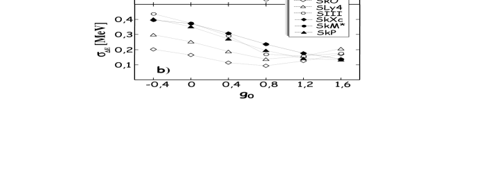
Figure 5: The average difference $\overline{\Delta E}$ ($\Delta E\equiv\Delta E_{exp}-\Delta E_{th}$) (upper part) and standard deviation $\sigma$ (lower part) between the data and the calculations versus Landau parameter $g_{0}$.

V The spin-orbit term

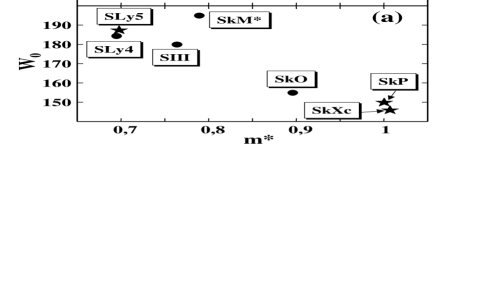
Figure 6: The strength $W_{0}$ (lower part) and the effective-mass scaled strength $W_{0}^{\star}$ (upper part) of the isoscalar part of the spin-orbit shf  potential versus the effective mass. Filled dots denote parameterizations which do not include tensor densities while those including these terms are indicated by stars. See text for more detail.

Within the shf theory, the $\ell s$-potential takes the following form:

$$V_{LS}(q,\bm{r})=-i\bm{W}_{q}(\bm{r})\bm{\nabla}\times\bm{\sigma},$$ (11)

where

$$\bm{W}_{q}(\bm{r})=\frac{1}{2}W{\bm{\nabla}}\rho_{0}(\bm{r})+\frac{1}{2}W^{\,\prime}{\bm{\nabla}}\rho_{q}(\bm{r})-\frac{1}{8}\left[(t_{1}x_{1}+t_{2}x_{2})\bm{J}(\bm{r})+(t_{2}-t_{1})\bm{J}_{q}(\bm{r})\right].$$ (12)

The vector spin density $\bm{J}(\bm{r})$ dependent terms appear to contribute rather weakly to the $\ell s$-potential. Hence, the magnitude of the $\ell s$-potential is determined essentially by the first two terms in Eq. (12). For the spherical limit the $\ell s$-potential can be approximated by:

$$V_{LS}(q,r)\approx\left\{W\frac{1}{r}\rho_{0}^{\,\prime}(r)+W^{\,\prime}\frac{1}{r}\rho_{q}^{\,\prime}(r)\right\}{\bm{\ell}}{\bm{s}}=\left\{\frac{W_{0}}{r}\rho_{0}^{\,\prime}(r)\pm\frac{W_{1}}{r}\rho_{1}^{\,\prime}(r)\right\}{\bm{\ell}}{\bm{s}}$$ (13)

where $\rho_{0}^{\,\prime}=(\rho_{n}+\rho_{p})^{\,\prime}$ and $\rho_{1}^{\,\prime}=(\rho_{n}-\rho_{p})^{\,\prime}$ are the radial derivatives of the local isoscalar and isovector densities, while $W_{0}\equiv W+\frac{1}{2}W^{\,\prime}$ and $W_{1}\equiv\frac{1}{2}W^{\,\prime}$ denote the isoscalar and isovector strengths, respectively.

A direct comparison of the isoscalar strengths $W_{0}$ of the $\ell s$-potential is given in Fig. 6a. Apparently, SLy4, Sly5, SkM^∗, and SIII forces have strong, while SkO, SkP, and SkXc have a weak $\ell s$-potential assuming, of course, that there are no drastic differences in the isoscalar density profile. The latter assumption should be rather well fulfilled in light nuclei, which are considered here. It is interesting to note that the conclusions stemming from a direct comparison of $W_{0}$ are in complete contradiction to the results presented in Fig. 4. Indeed, according to our calculations Sly4, SLy5, SkO, SIII, and eventually also SkXc are expected to have similar $\ell s$-strength while it should be considerably stronger for SkM^∗ and SkP.

The question therefore arises of how to compare the strengths of the $\ell s$-potential for different parameterizations. The problem appears to be related to non-local effects which are, within the shf, absorbed into the kinetic energy term through the effective mass $m^{*}$. The impact of non-localities on the $\ell s$-potential can be studied using the so called asymptotically equivalent wave function [Bei75] ; [Lop00]

$$\tilde{\phi}_{i}(\bm{r})=\sqrt{\frac{m}{m^{\star}(\bm{r})}}\phi_{i}(\bm{r}).$$ (14)

This representation allows to rewrite the shf equations in an alternative form with a bare mass $m$ in the kinetic energy term, a state-dependent central potential $U_{q}(e_{\mu};\bm{r})$, and the effective-mass-scaled $\ell s$-potential (13):

$$V_{LS}(q,r)\approx\frac{m^{\star}(r)}{m}\left\{\frac{W_{0}}{r}\rho_{0}^{\,\prime}(r)\pm\frac{W_{1}}{r}\rho_{1}^{\,\prime}(r)\right\}{\bm{\ell}}{\bm{s}}.$$ (15)

The effective-mass-scaled isoscalar strengths $W_{0}^{*}\equiv\frac{m^{\star}}{m}W_{0}$ are depicted in Fig. 6b. Note, that the classification of the $\ell s$-strength according to $W_{0}^{*}$ agrees very nicely with our results shown in Fig. 4. Indeed, the values of $W_{0}^{*}$ are similar for Sly4, SLy5, SIII, and SkO and considerably larger for SkP and SkM^∗.

This indicates that at least part of the observed discrepancy, $\overline{\Delta E}$, results from a too strong $\ell s$-term. By reducing the strength with $\sim 5$%, the $\overline{\Delta E}$ reduces by $\sim$350 keV bringing it to an acceptable level of $\overline{\Delta E}\sim 200$ keV for most of the forces. In particular, for the case of the SkO force $\overline{\Delta E}$ drops from 504 keV to 164 keV, while for Sly4 a 5% reduction of the $\ell s$-strength decreases $\overline{\Delta E}$ from 560 keV to 189 keV.

Concerning the isovector $\ell s$-potential, the Skyrme forces which are discussed in the literature can be divided into three major classes. The standard Skyrme force parameterizations assume that $W=W^{\,\prime}$ ($W_{1}/W_{0}=1/3$), implying that ${\bm{W}}_{q}\sim W(2\rho_{q}^{\,\prime}+\rho_{-q}^{\,\prime})$. The Sly4, Sly5, SkM^∗, SkO, and SIII are standard forces among those studied here.

Non-standard Skyrme interactions with $W\neq W^{\,\prime}$ were first studied by Reinhard and Flocard [Rei95] in connection with isotope shifts in Pb nuclei. Consistency with experimental data led them to the parameterizations with $W^{\,\prime}\sim-W$ or ($W_{1}/W_{0}=-1$), i.e. to an entirely different isovector dependence of the $\ell s$-term ${\bm{W}}_{q}\sim W\rho_{-q}^{\,\prime}$ as compared to the standard one. The study of the $\ell s$-term in neutron-rich nuclei by Reinhardt et al. [Rei99] seems further to corroborate this result. The so called SkO parametrization established in Ref. [Rei99] (and studied here) have even larger negative value of $W_{1}$ with $W_{1}/W_{0}\approx-1.3$.

The third type of the $\ell s$-term which is considered in the literature in connection with the shf approach, was introduced by Brown [Bro98] who uses $W^{\,\prime}=0$ (parametrization SkXc). In this case there is no isovector $\ell s$-term ($W_{1}/W_{0}\equiv 0$) and ${\bm{W}}_{q}\sim W(\rho_{n}^{\,\prime}+\rho_{p}^{\,\prime})$.

Figure 7: The values of $\Delta E$ calculated using SkO-induced l-ledf with four different parameterizations of the isovector $\ell s$-term, including the original $W_{1}/W_{0}\approx-1.3$ strength and the modified strengths $W_{1}/W_{0}=-1,0,1/3$. In the calculations $W_{0}$ was kept fix at 5% below its original value. The insert shows the dependence of the spread in $\Delta E$, $\sigma_{\Delta E}$, on $W_{1}/W_{0}$ calculated for SkO-induced as well as SLy4-induced l-ledf.

As already discussed at the end of Sect. IV.2 our calculations give certain preference for the SkO-induced l-ledf, since it minimizes the spread in $\Delta E$, $\sigma_{\Delta E}$. In particular, this result seems to speak in favor of a $\ell s$-potential with large negative isovector strength $W_{1}$. To reinforce this observation we have performed a set of calculations based on SkO-induced l-ledf, but exploring different isovector dependence of the $\ell s$-term, including the four possibilities discussed above $W_{1}/W_{0}=-1.3,-1,0,1/3$. In the calculations, the isoscalar strength $W_{0}$ was kept constant and its value was reduced by 5% as compared to the original SkO strength.

The calculated values of $\Delta E$ for these four variations of the SkO-induced l-ledf are shown in Fig. 7. Drastic change in the $W_{1}/W_{0}$ ratio from the (near)original values –1.3, –1 to 0, 1/3 clearly destroy the agreement to the data. Indeed, the spread, $\sigma_{\Delta E}$, increases from 113 keV and 136 keV ($W_{1}/W_{0}=-1.3,-1$) to 184 keV and 180 keV ($W_{1}/W_{0}=1/3,\,0$), respectively, see insert in Fig. 7. Note, however, that since we deal with $N$$\sim$$Z$, a fine tuning of the isovector terms cannot be achieved.

Similar calculations, but with the SLy4-induced l-ledf additionally corroborate our conclusions. The change in $W_{1}/W_{0}$ ratio from the (near)original values 1/3, 0 to –1, –1.3 improve the agreement to the data, as shown in the insert in Fig. 7. Note also, that the calculated spread, $\sigma_{\Delta E}$, is quantitatively very similar for both the SkO-induced and SLy4-induced l-ledf provided the isovector part of the $\ell s$-term is similar.

VI $2p$-$2h$ terminating state in ⁴⁵Sc and the additivity of $1p$-$1h$ excitations.

The $2p$-$2h$ $d_{3/2}^{-2}f_{7/2}^{n+2}$ terminating states can provide further insight into the to terms, the $\ell s$ potential, and into various polarization phenomena, since they allow to test self-consistent calculations against simple, intuitive additivity relations. Thus far such state is known, however, only in ⁴⁵Sc [Lenzi] . Although a single case does not allow for deep conclusions, the comparison between the data and the calculations, see Fig. 8, clearly shows that some naively-understood additivity concepts do not always work.

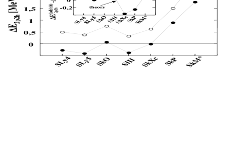
Figure 8: $\Delta E_{2p2h}$ calculated for different Skyrme-force-induced l-ledf. Open circles mark calculations using the standard $\ell s$ strength, while those using a 5% reduced $\ell s$ strength are labeled by filled circles. The insert shows the theoretically calculated deviation from the additivity $\Delta E_{2p2h}^{(add;th)}-\Delta E_{2p2h}^{(th)}$. The corresponding experimental value of $\Delta E_{2p2h}^{(add;exp)}-\Delta E_{2p2h}^{(exp)}$=0.252 MeV is marked by a solid line.

For example, the values of $\Delta E_{2p2h}\equiv\Delta E_{2p2h}^{(exp)}-\Delta E_{2p2h}^{(th)}$ calculated using Sly4, SLy5, SIII, and SkXc l-ledf are comparable or even smaller than the corresponding values of $\Delta E$ obtained for the terminating $1p$-$1h$ state in ⁴⁵Sc, see Fig. 4. Consequently, calculations using a 5% reduced isoscalar $\ell s$-strength overestimate the data with exception of the SkXc l-ledf for which one obtains an almost perfect agreement to the data. On the contrary, the additivity seems to work perfectly for the SkO-induced l-ledf. A reduction of the $\ell s$-strength by 5% gives, in this case, an excellent agreement to the data.

The excitation energy of the $2p$-$2h$ terminating state in ⁴⁵Sc can be approximated by a sum of the energy of the two aligned $29/2^{+}$, $[d_{3/2}^{-1}f_{7/2}^{n+1}]_{(I_{max}-1)}$ states terminating at unfavored signature. Since there exist exactly two such states, their centroid energy (sum of their energies) should be fairly insensitive to the possible beyond-mean-field mixing effects. Hence, the additivity relation for the excitation energies should provide an independent characteristics of the ledf.

Insert in Fig. 8 shows the theoretically calculated difference $\Delta E_{2p2h}^{(add;th)}-\Delta E_{2p2h}^{(th)}$ where $\Delta E_{2p2h}^{(th)}$ denotes excitation energy of the terminating $2p$-$2h$ state while $\Delta E_{2p2h}^{(add;th)}$ denotes $2p$-$2h$ excitation energy calculated by adding excitation energies of the two $1p$-$1h$ configurations given above. In general, the additivity works relatively well. There are however two exceptions: the SkP and, unexpectedly, SkXc l-ledf. The downward shift of SLy5 with respect to SLy4 as well as rather mediocre agreement for SkP and SkXc forces, may be is related to the tensor component that is present in these three forces and deserves further investigation.

This short analysis indicates already the rich physics that can be addressed using $2p$-$2h$ terminating states.

VII Summary

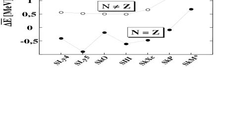
Figure 9: The average deviation $\overline{\Delta E}$ for $N$$\neq$$Z$ (open dots) and for $N$$=$$Z$ (filled dots) nuclei. The latter case includes data in ⁴⁴Ti [Lenzi] where $E[f_{7/2}^{n}]_{12^{+}}$=8.038 MeV, $E[d_{3/2}^{-1}f_{7/2}^{n+1}]_{15^{-}}$=13.369 MeV, and $\Delta E_{exp}$=5.331 MeV, and ⁴⁶V [Len99] where $E[f_{7/2}^{n}]_{15^{+}}$=8.484 MeV, $E[d_{3/2}^{-1}f_{7/2}^{n+1}]_{17^{-}}$=13.629 MeV, and $\Delta E_{exp}$=5.145 MeV. All calculations were done using l-ledf.

We have performed a systematic study of terminating states in the $A$$\sim$50 mass region using the self-consistent Skyrme-Hartree-Fock model and testing several parameterizations of the Skyrme force. The objective was to demonstrate that the terminating states, due to their intrinsic simplicity, offer an unique and so far unexplored opportunity to study different aspects of effective NN interaction or nuclear local energy density functional within the self-consistent approaches.

It is shown, that the Skyrme-force parameterizations used in our work, including Sly4, Sly5, SkO, SIII, SkXc, SkP, and SkM^∗, give rise to a rather mediocre (for SkP and SkM^∗ even unacceptable) agreement with the data even for such a seemingly simple observable like the energy difference between the aligned $f_{7/2}^{n}$ and $d_{3/2}^{-1}f_{7/2}^{n+1}$ states.

It is further demonstrated that a simple unification of the spin fields according to the scheme proposed in Ref. [Ben02] leads to an unified description of the data for Sly4, Sly5, SkO, SIII, SkXc, i.e. for very different parameterizations. This result seems to indicate the importance of the local gauge (and Galilean) invariance of the local energy density functional. The remaining discrepancy of $\sim$500 keV (see Fig. 9) which is still of the order of $\sim$10% cannot be reduced by further readjusting the spin fields.

It is also shown, that the observed disagreement between theory and experiment for different parameterizations correlates nicely with the values of the effective mass scaled isoscalar strength of the $\ell s$-term for these parameterizations. Hence, a part of this discrepancy can, most likely, be ascribed to a too strong isoscalar $\ell s$-term. Reduction of the isoscalar $\ell s$-strength by 5% reduces the discrepancy well below the 5% level. Moreover, our calculations suggest that the spread in $\Delta E$ can be further reduced by adopting the non-standard parameterizations of the $\ell s$-term with a strong negative isovector strength $W_{1}/W_{0}\leq-1$.

Finally, let us point out that there is a large difference in $\overline{\Delta E}$ calculated in $N$$\neq$$Z$ and $N$$=$$Z$ nuclei, see Fig. 9. For $N$$\neq$$Z$ our l-ledf approach systematically underestimates the data while the opposite is true for $N$$=$$Z$ nuclei. The offset between the two curves is of the order of $\sim$1 MeV. This result leaves us with an extremely important question: Does this offset indicate a breakdown of the standard mean-field in $N$$\sim$$Z$ nuclei and a need for substantial configuration mixing even at the terminating states [Ter98] and what is the possible source of such mixing?

This work was supported by the Foundation for Polish Science (FNP), the Göran Gustafsson Foundation, the Swedish Science Council (VR), the Swedish Institute (SI) and the Polish Committee for Scientific Research (KBN). The authors thank Sylvia Lenzi and Jan Styczeń for communicating experimental results prior to publication. One of us (WS) is grateful to J. Dobaczewski for stimulating discussions and many constructive comments on the manuscript.

References

- (1) K. Rutz, M. Bender, P.-G. Reinhard, J.A. Maruhn, and W. Greiner, Nucl. Phys. A634 (1998) 67.
- (2) M. Lopez-Quelle, N. Van Giai, S. Marcos, and L.N. Savushkin, Phys. Rev. C61 (2000) 064321.
- (3) I. Hamamoto and P.Siemens, Nucl. Phys. A269 (1976) 199.
- (4) V. Bernard and N. van Giai, Nucl. Phys. A348 (1980) 75.
- (5) A. Oros, Ph.D. thesis, University of Köln, 1996.
- (6) A. Swift and L.R.B. Elton, Phys. Rev. Lett. 17 (1966) 484.
- (7) H. Tyren, S. Kullander, O. Sundberg, R. Ramachandran, P. Isacsson, and T. Berggren, Nucl. Phys. 17 (1966) 321.
- (8) L. Ray and P.E. Hodgson, Phys. Rev. C20 (1979) 2403.
- (9) V.I. Isakov, K.I. Erokhina, H. Mach, M. Sanchez-Vega, and B. Fogelberg, Eur. Phys. J. A14 (2002) 29.
- (10) S.G. Nilsson, Mat. Fys. Medd. Dan. Vid. Selsk. 29 (1955).
- (11) A. Bohr, B. Mottelson, and I. Hamamoto, Phys. Scr. 26 (1982) 267.
- (12) C. Bahri, J.P. Draayer, and S.A. Moszkowski, Phys. Rev. Lett. 68 (1992) 2133.
- (13) J. Ginocchio, Phys. Rev. Lett. 78 (1997) 436.
- (14) A.V. Afanasjev, D.B. Fossan, G.J. Lane, and I. Ragnarsson, Phys. Rep. 322, 1 (1999).
- (15) W. Satuła and R. Wyss, submitted to Rep. Prog. Phys. (2004).
- (16) J. Dobaczewski and J. Dudek, Comput. Phys. Commun. 131 (2000) 164.
- (17) J. Dobaczewski, J. Dudek, and P. Olbratowski, Comput. Phys. Commun. 158 (2004) 158; HFODD user’s guide, to be published.
- (18) M. Lach, J. Styczeń, W. Mȩczyński, P. Bednarczyk, A. Bracco, J. Grȩbosz, A. Maj, J.C. Merdinger, N. Schulz, M.B. Smith, K.M. Spohr, J.P. Vivien, and M. Ziȩbliński, Eur. Phys. J. A16 (2003) 309.
- (19) S. Lenzi and J. Styczeń, private communication.
- (20) M. Lach, J. Styczeń, W. Mȩczyński, P. Bednarczyk, A. Bracco, J. Grȩbosz, A. Maj, J.C. Merdinger, N. Schulz, M.B. Smith, K.M. Spohr, and M. Ziȩbliński, Eur. Phys. J. A (2004) in print.
- (21) P. Bednarczyk et al., Acta Phys. Pol. B32 (2001) 747.
- (22) F. Brandolini, N.H. Medina, S. Lenzi, D.R. Napoli, A. Poves, R.V. Ribas, J. Sanchez-Solano, C.A. Ur, M. De Poli, N. Marginean, D. Bazzacco, J.A. Cameron, G. de Angelis, A. Gadea, N. Menegazzo, and C. Rossi-Alvarez, Nucl. Phys. A693 (2001) 517.
- (23) W. Satuła et al., to be published.
- (24) J. Dobaczewski and J. Dudek, Phys. Rev. C52, 1827 (1995); C55 (1997) E3177.
- (25) M. Bender, J. Dobaczewski, J. Engel, and W. Nazarewicz, Phys. Rev. C65, 054322 (2002).
- (26) Y.M. Engel, D.M. Brink, K. Goeke, S.J. Krieger, and D. Vautherin, Nucl. Phys. A249, 215 (1975).
- (27) P. Hohenberg and W. Kohn, Phys. Rev. 136 (1964) B864.
- (28) W. Kohn and L.J. Sham, Phys. Rev. 140 (1965) A1133.
- (29) W. Kohn, Rev. Mod. Phys. 71 (1998) 1253.
- (30) J. Dobaczewski, H. Flocard, and J. Treiner, Nucl. Phys. A422 (1984) 103.
- (31) B.A. Brown, Phys. Rev. C58 (1998) 220.
- (32) E. Chabanat, P. Bonche, P. Haensel, J. Meyer, and F. Schaeffer, Nucl. Phys. A627 (1997) 710; A635 (1998) 231.
- (33) M. Beiner, H. Flocard, N. Van Giai, and P. Quentin, Nucl. Phys. A422 (1975) 29.
- (34) P.-G. Reinhard, D.J. Dean, W. Nazarewicz, J. Dobaczewski, J.A. Maruhn, and M.R. Strayer, Phys. Rev. C60 (1999) 014316.
- (35) J. Bartel, P. Quentin, M. Brack, C. Guet, and H.B. Håkansson, Nucl. Phys. A386, 79 (1982).
- (36) F. Osterfeld, Rev. Mod. Phys. 64 (1992) 491.
- (37) W. Satuła, in Nuclear Structure 98, ed. by C. Baktash, AIP Conf. Proc. No. 481, (AIP, Woodbury, NY, 1999), p. 114; nucl-th/9809089.
- (38) P.-G. Reinhard and H. Flocard, Nucl. Phys. A584, 467 (1995).
- (39) S. Lenzi, D.R. Napoli, C.A. Ur, D. Bazzacco, F. Brandolini, J.A. Cameron, E. Caurier, G. de Angelis, M. De Poli, E. Farnea, A. Gadea, S. Hankonen, S. Lunardi, G. Martinez-Pinedo, Zs. Podolyak, A. Poves, C. Rossi-Alvarez, J. Sanchez-Solano, and H. Sornacal, Phys. Rev. C60 (1999) 021303.
- (40) J. Terasaki, R. Wyss, and P.-H. Heenen, Phys. Lett. B437 (1998) 1.