The Kinetic Energy Density in Kohn-Sham
Density Functional Theory

Abstract

This work continues a program to systematically generalize the Skyrme Hartree-Fock method for medium and heavy nuclei by applying effective field theory (EFT) methods to Kohn-Sham density functional theory (DFT). When conventional Kohn-Sham DFT for Coulomb systems is extended beyond the local density approximation, the kinetic energy density $\tau$ is sometimes included in energy functionals in addition to the fermion density. However, a local (semi-classical) expansion of $\tau$ is used to write the energy as a functional of the density alone, in contrast to the Skyrme approach. The difference is manifested in different single-particle equations, which in the Skyrme case include a spatially varying effective mass. Here we show how to generalize the EFT framework for DFT derived previously to reconcile these approaches. A dilute gas of fermions with short-range interactions confined by an external potential serves as a model system for comparisons and for testing power-counting estimates of new contributions to the energy functional.

I Introduction

Density functional theory (DFT) is widely used in many-body applications with Coulomb interactions because it provides a useful balance between accuracy and computational cost, allowing large systems to be treated in a simple self-consistent manner. In DFT, the particle density $\rho{({\bf\bf{x}})}$ plays a central role rather than the many-body wave function. DFT has the generality to deal with any interaction but has had little explicit impact on nuclear structure phenomenology so far (see, however Refs. PETKOV91 ; HOFMANN98 ; Fayans:2001fe ; SOUBBOTIN03 ), although the Skyrme-Hartree-Fock formalism is often considered to be a form of DFT BRACK85 . In previous work, effective field theory (EFT) methods were applied in a DFT framework, with the ultimate goal of calculating bulk observables for medium to heavy nuclei in a systematic fashion. The present work takes another step toward this goal by generalizing the EFT framework for DFT to include the kinetic energy density in the same way it appears in the Skyrme approach.

Kohn-Sham (KS) DFT maps an interacting many-body system to a much easier-to-solve non-interacting system. Hohenberg and Kohn proved that the ground-state density $\rho{({\bf\bf{x}})}$ of a bound system of interacting particles in some external potential $v({\bf\bf{x}})$ determines this potential uniquely up to an additive constant HK64 . They showed that there exists an energy functional $E[\rho]$ that can be decomposed as

$$E[\rho({\bf\bf{x}})]=F_{\rm HK}[\rho({\bf\bf{x}})]+\int\!d^{3}{\bf\bf{x}}\,v({\bf\bf{x}})\rho({\bf\bf{x}})\ ,$$ (1)

where the functional $F_{\rm HK}[\rho]$ is called the HK free energy, and is universal in the sense that it has no explicit dependence on the potential $v({\bf\bf{x}})$. A variational principle, formulated in terms of trial densities rather than trial wavefunctions, ensures that the functional $E[\rho]$ is a minimum equal to the ground-state energy when evaluated at the exact ground-state density.

The free-energy functional $F_{\rm HK}[\rho]$ can be further decomposed into a non-interacting kinetic energy $T_{s}[\rho]$, the Hartree term $E_{H}[\rho]$, and the exchange-correlation energy $E_{xc}[\rho]$ ARGAMAN00 :

$$F_{\rm HK}[\rho]=T_{s}[\rho]+E_{H}[\rho]+E_{xc}[\rho]\ .$$ (2)

Kohn-Sham DFT KOHN65 ; PARR89 ; DREIZLER90 ; KOHN99 ; ARGAMAN00 allows $T_{s}[\rho]$ to be calculated exactly [see Eq. (30)], which efficiently treats a leading source of non-locality in the energy functional. Given the Hartree and exchange-correlation functionals, the solution of the interacting problem at zero temperature reduces to solving a single-particle Schrödinger equation,

$$\bigl{[}-\frac{{\nabla}^{2}}{2M}+v_{s}({\bf\bf{x}})\bigr{]}\,\psi_{\beta}({\bf x})=\varepsilon_{\beta}\psi_{\beta}({\bf x})\,,$$ (3)

for the lowest $A$ orbitals $\psi_{\beta}({\bf\bf{x}})$ (including degeneracies), where the effective local external potential $v_{s}({\bf\bf{x}})$ is given by

$$v_{s}({\bf\bf{x}})=v({\bf\bf{x}})+\frac{\delta E_{H}[\rho]}{\delta\rho{({\bf\bf{x}})}}+\frac{\delta E_{xc}[\rho]}{\delta\rho{({\bf\bf{x}})}}\,.$$ (4)

The wave functions for the occupied states in this fictitious external potential $v_{s}({\bf\bf{x}})$ generate the same physical density $\rho{({\bf\bf{x}})}$ through $\rho({\bf\bf{x}})\equiv\sum_{\beta}|\psi_{\beta}({\bf\bf{x}})|^{2}$ as that of the original, fully interacting system in the external potential $v({\bf\bf{x}})$.

The practical problem of DFT is finding a useful explicit expression for $E_{xc}[\rho]$ DREIZLER90 ; PARR89 ; ARGAMAN00 ; KOHN99 . For Coulomb systems, the conventional procedure is to approximate $E_{xc}$ in the local density approximation (LDA) by taking the exchange-correlation energy density at each point in the system to be equal to its value for a uniform interacting system at the local density (which is calculated numerically) ARGAMAN00 , and then to include semi-phenomenological gradient corrections PERDEWWANG92 ; ARGAMAN00 . These gradient corrections have become steadily more sophisticated. The initial attempts at gradient corrections violated a sum rule KOHN99 ; ARGAMAN00 , which was fixed by the generalized gradient expansion approximation (GGA), where spatial variations of $\rho({{\bf\bf{x}}})$ are constrained by construction to conform with the sum rule PERDEW96 . To further improve the exchange-correlation functional, the semi-local kinetic energy density $\tau{({\bf\bf{x}})}\equiv\sum_{\beta}|\bm{\nabla}\psi_{\beta}({\bf\bf{x}})|^{2}$ was built into the GGA formalism to construct meta-generalized gradient approximations (Meta-GGA) PERDEW99 . However, in practice, the kinetic energy density is replaced by its local expansion in terms of the density $\rho({{\bf\bf{x}}})$ and its gradients DREIZLER90 so that the energy is treated as a functional of the density alone. The Kohn-Sham single-particle equation still takes the form of Eq. (3).

The Skyrme-Hartree-Fock approach to nuclei is also based on energy functionals and single-particle equations, which suggests a link between the traditional DFT and nuclear mean-field approaches BRACK85 ; SCHMID95 ; SCHMID95a . In calculations with the usual density-dependent Skyrme force, the energy density for spherical, even-even $N=Z$ nuclei takes the form of a local expansion in density VB72 ; RINGSCHUCK ,

$${\cal E}_{SK}{({\bf\bf{x}})} = \frac{1}{2M}\tau{({\bf\bf{x}})}+\frac{3}{8}t_{0}{[\rho{({\bf\bf{x}})}]}^{2}+\frac{1}{16}t_{3}{[\rho{({\bf\bf{x}})}]}^{2+\alpha}+\frac{1}{16}(3t_{1}+5t_{2})\rho{({\bf\bf{x}})}\,\tau{({\bf\bf{x}})}$$ (5)

$$+\frac{1}{64}(9t_{1}-5t_{2})|\bm{\nabla}\rho({\bf\bf{x}})|^{2}-\frac{3}{4}W_{0}\rho{({\bf\bf{x}})}\bm{\nabla}\cdot\bm{J}({\bf\bf{x}})+\frac{1}{32}(t_{1}-t_{2})[{\bm{J}}({\bf\bf{x}})]^{2}\,,$$

(see Ref. JACEK95 for a more general treatment). The density $\rho$, kinetic density $\tau$, and the spin-orbit density $\bm{J}$ are expressed as sums over single-particle orbitals $\psi_{\beta}({\bf\bf{x}})$:

$$\rho({\bf\bf{x}})\equiv\sum_{\beta}|\psi_{\beta}({\bf\bf{x}})|^{2}\,,\qquad\tau({\bf\bf{x}})\equiv\sum_{\beta}|\bm{\nabla}\psi_{\beta}({\bf\bf{x}})|^{2}\,,\qquad\bm{J}({\bf\bf{x}})\equiv\sum_{\beta}\psi^{\dagger}_{\beta}({\bf\bf{x}})(\bm{\nabla\times\sigma})\psi_{\beta}({\bf\bf{x}})\,,$$ (6)

where the sums are over occupied states. The $t_{i}$’s, $W_{0}$, and $\alpha$ are generally obtained from numerical fits to experimental data. Varying the energy with respect to the wavefunctions leads to a Schrödinger-type equation with a position-dependent mass term VB72 ; RINGSCHUCK :

$$\Bigl{(}-\bm{\nabla}\frac{1}{2M^{*}({\bf\bf{x}})}\bm{\nabla}+U({\bf\bf{x}})+W({\bf\bf{x}})\Bigr{)}\,\psi_{\beta}({\bf\bf{x}})=\varepsilon_{\beta}\,\psi_{\beta}({\bf\bf{x}})\,,$$ (7)

where $M^{*}({\bf\bf{x}})$ is given by

$$\frac{1}{2M^{*}({\bf\bf{x}})}=\frac{1}{2M}+\left[{3\over{16}}\,t_{1}+{5\over{16}}\,t_{2}\right]\,\rho({\bf\bf{x}})\,,$$ (8)

and $W({\bf\bf{x}})$ is a spin-orbit potential (see Ref. JACEK95 for details). The appearance of $M^{*}({\bf\bf{x}})$ and $W({\bf\bf{x}})$ are a consequence of not expanding $\tau$ and $\bm{J}$ in terms of $\rho$.

The Skyrme approach has had many phenomenological successes over the last 30 years and, generalized to include the effects of pairing correlations, continues to be a major tool for analyzing the nuclear structure of medium and heavy nuclei BROWN98 ; Dobaczewski:2001ed ; BENDER2003 ; Stoitsov:2003pd . The form of the Skyrme interaction was originally motivated as an expansion of an effective interaction (G-matrix) in the medium SKYRME . Negele and Vautherin made the connection concrete with the density matrix expansion method DME , but there has been little further development since their work. Many unresolved questions remain, which become acute as one attempts to reliably extrapolate away from well-calibrated nuclei and to connect to modern treatments of the few-nucleon problem. Why are certain terms included in the energy functional and not others? What is the expansion parameter(s)? How can we estimate uncertainties in the predictions? Are long-range effects included adequately? Can we really include correlations beyond mean-field, as implied by the DFT formalism? We turn to effective field theory to address these questions, using a DFT rather than a G-matrix approach as in Ref. Duguet:2002xn .

Effective field theory (EFT) promises a model-independent framework for analyzing low-energy phenomena with reliable error estimates EFT98 ; EFT99 ; LEPAGE89 ; Birareview ; BEANE99 . In Ref. PUG02 , an effective action framework was used to merge effective field theory with DFT for a dilute gas of identical fermions confined in an external potential with short-range, spin-independent interactions (see also Refs. Polonyi:2001uc ; Schwenk:2004hm ). The calculations in Ref. PUG02 used the results from the EFT treatment of a uniform system in Ref. HAMMER00 in the local density approximation. In the present work, we extend the formalism to include the kinetic energy density as a functional variable, leading to Kohn-Sham equations with position-dependent $M^{*}$’s (see Ref. AUREL95 for an earlier discussion of such an extension to Kohn-Sham DFT). We take a (small) step beyond the LDA by evaluating the full $\tau$ dependence in the Hartree-Fock diagrams with two-derivative vertices, which leads to an energy expression similar to the standard Skyrme energy (excepting the spin-orbit parts).

The plan of the paper is as follows. In Sect. II, we extend the EFT/DFT construction for a dilute Fermi system to include a source coupled to the kinetic energy density operator. A double Legendre transformation, carried out via the inversion method, yields an energy functional of $\rho$ and $\tau$, and Kohn-Sham equations with $M^{*}({\bf\bf{x}})$. In Sect. III, we illustrate the formalism with numerical calculations for a dilute Fermi system in a trap, including power-counting estimates. Section IV is a summary. For the bulk of the paper, we will restrict our discussion to spin-independent interactions but in Sec. II.4 the extension to more general forces is discussed.

II EFT/DFT with the Kinetic Energy Density

A dilute Fermi system with short-range interactions is an ideal test laboratory for effective field theory at finite density, but it is also directly relevant for comparison to Skyrme functionals. We describe such a system using a general local Lagrangian for a nonrelativistic fermion field with spin-independent, short-range interactions that is invariant under Galilean, parity, and time-reversal transformations BEANE99 ; HAMMER00 :

$${\cal L} = \psi^{\dagger}\biggl{[}i\partial_{t}+\frac{\overrightarrow{\nabla}^{\,2}}{2M}\biggr{]}\psi-\frac{C_{0}}{2}(\psi^{\dagger}\psi)^{2}+\frac{C_{2}}{16}\Bigl{[}(\psi\psi)^{\dagger}(\psi\tensor{\nabla}^{2}\psi)+\mbox{ h.c.}\Bigr{]}$$ (9)

$$\hbox{}+\frac{C_{2}^{\prime}}{8}(\psi\tensor{\nabla}\psi)^{\dagger}\cdot(\psi\tensor{\nabla}\psi)+\cdots\ ,$$

where $\tensor{\nabla}=\overleftarrow{\nabla}-\overrightarrow{\nabla}$ is the Galilean invariant derivative and h.c. denotes the Hermitian conjugate. The terms proportional to $C_{2}$ and $C_{2}^{\prime}$ contribute to $s$-wave and $p$-wave scattering, respectively, while the dots represent terms with more derivatives and/or more fields. To describe trapped fermions, we add to the Lagrangian a term for an external confining potential $v({\bf\bf{x}})$ coupled to the density operator $v({\bf\bf{x}})\psi^{\dagger}\psi$ PUG02 . For the numerical calculations, we take the potential to be an isotropic harmonic confining potential,

$$v({\bf\bf{x}})={1\over 2}m\,\omega^{2}\,|{\bf\bf{x}}|^{2}\ ,$$ (10)

although the discussion holds for a general non-vanishing external potential. This Lagrangian can be simply generalized to include spin-dependent interactions, as described in Sec. II.4, although the complete set of terms grows rapidly with the number of derivatives.

II.1 Effective Action and the Inversion Method

We introduce a generating functional in the path integral formulation with ${\cal L}$ from Eqs. (9) and (10) supplemented by c-number sources $J(x)$ and $\eta(x)$, coupled to the composite density operator and to the kinetic energy density operator, respectively,

$$Z[J,\eta]=e^{iW[J,\eta]}=\int\!D\psi D\psi^{\dagger}\ e^{i\int\!d^{4}x\ [{\cal L}\,+\,J(x)\psi^{\dagger}(x)\psi(x)\,+\,\eta(x)\bm{\nabla}\psi^{\dagger}(x)\cdot\bm{\nabla}\psi(x)]}\ .$$ (11)

For simplicity, normalization factors are considered to be implicit in the functional integration measure FUKUDA94 ; FUKUDA95 . The fermion density in the presence of the sources is

$$\rho(x)\equiv\langle\psi^{\dagger}(x)\psi(x)\rangle_{J\,,\,\eta}={\delta W[J,\eta]\over\delta J(x)}\ ,$$ (12)

and the kinetic energy density is given by

$$\tau(x)\equiv\langle\bm{\nabla}\psi^{\dagger}(x)\bm{\cdot\nabla}\psi(x)\rangle_{J\,,\,\eta}={\delta W[J,\eta]\over\delta\eta(x)}\ ,$$ (13)

where functional derivatives are taken keeping the other source fixed. The effective action is defined through the functional Legendre transformation

$$\Gamma[\rho,\tau]=W[J,\eta]-\int\!d^{4}x\,J(x)\rho(x)-\int\!d^{4}x\,\eta(x)\tau(x)\ ,$$ (14)

which implies that $\Gamma$ has no explicit dependence on $J$ and $\eta$.

As in Ref. PUG02 , we choose finite-density boundary conditions that enforce a given particle number $A$ by hand, so that $\Gamma$ and $W$ are functions of $A$ and variations over $\rho(x)$ and $\tau(x)$ conserve $A$. This is naturally achieved by working with a fixed number of Kohn-Sham orbitals, as seen below. By limiting ourselves to time independent sources and densities, we can factor out a ubiquitous time factor corresponding to the time interval over which the source is acting, and write PUG02

$${\widetilde{\Gamma}}[\rho,\tau]\equiv\Gamma[\rho,\tau]\times\left[\int_{-\infty}^{\infty}\,dt\right]^{-1}=-E[\rho,\tau]\,.$$ (15)

and similarly with $W[J,\eta]$ and the expansions below. The effective action has extrema at the possible quantum ground states of the system, and when evaluated at the minimum is proportional (at zero temperature) to the ground-state energy FUKUDA94 ; FUKUDA95 ; HU96 . In particular, Eq. (15) defines an energy functional $E[\rho,\tau]$, which when evaluated with the exact ground-state density $\rho$ and kinetic energy density $\tau$, is equal to the ground-state energy.

If we take functional derivatives of Eq. (14) with respect to $J({\bf\bf{x}})$ and $\eta({\bf\bf{x}})$, and then apply Eqs. (12) and (13) PUG02 , we obtain two equations that can be written in matrix form as

$$\int d^{3}{\bf y}\,\left(\begin{array}[]{lr}\frac{\textstyle\delta\rho({\bf y})\phantom{{\widetilde{\Gamma}}}}{\textstyle\delta J({\bf\bf{x}})}&\frac{\textstyle\delta\tau({\bf y})}{\textstyle\delta J({\bf\bf{x}})}\\[10.0pt] \frac{\textstyle\delta\rho({\bf y})\phantom{{\widetilde{\Gamma}}}}{\textstyle\delta\eta({\bf\bf{x}})}&\frac{\textstyle\delta\tau({\bf y})}{\textstyle\delta\eta({\bf\bf{x}})}\end{array}\right)\,\left(\begin{array}[]{l}\frac{\textstyle\delta{\widetilde{\Gamma}}[\rho,\tau]}{\textstyle\delta\rho({\bf y})}+J({\bf y})\\[10.0pt] \frac{\textstyle\delta{\widetilde{\Gamma}}[\rho,\tau]}{\textstyle\delta\tau({\bf y})}+\eta({\bf y})\end{array}\right)=0\ .$$ (16)

The invertibility of the transformation from $\{J,\eta\}$ to $\{\rho,\tau\}$ implies that the matrix in Eq. (16) has no zero eigenvalues, which means that the elements of the vector vanish identically for each ${\bf\bf{x}}$, so that

$$\frac{\delta{\widetilde{\Gamma}}[\rho,\tau]}{\delta\rho({\bf\bf{x}})}=-J({\bf\bf{x}})\ ,\qquad\frac{\delta{\widetilde{\Gamma}}[\rho,\tau]}{\delta\tau({\bf\bf{x}})}=-\eta({\bf\bf{x}})\ .$$ (17)

Thus, the effective action when evaluated at the exact ground state density and kinetic energy density is an extremum when the sources are set to zero, which corresponds to the original (source-free) system. The convexity of $\Gamma$ implies that the energy (equal to minus ${\widetilde{\Gamma}}[\rho,\tau]$ at the extremum) is a minimum.

These properties are analogous to conventional applications of effective actions where the Legendre transformation is with respect to one of the fields rather than a composite operator COLEMAN88 ; PESKIN95 ; WEINBERG96 . A possible complication in the present case would be if new divergences arose in $W[J,\eta]$, which generally happens when adding a source coupled to a composite operator BANKSRABY ; COLLINS86 . However, that is not the case here FURNSTAHL04 . On the other hand, sources coupled to operators such as $\psi\psi+\psi^{\dagger}\psi^{\dagger}$, which arise when considering pairing, will introduce new divergences, including for the kinetic energy density. This issue will be considered elsewhere FURNSTAHL04 .

To carry out the inversion and Legendre transformation, we apply the inversion method of Fukuda et al. FUKUDA94 ; FUKUDA95 ; VALIEV96 ; VALIEV97 ; VALIEV97b ; RASAMNY98 . This method applies to any system that can be characterized by a hierarchy, which we organize by introducing a parameter $\lambda$ that is ultimately set to unity. This parameter can label different orders in a coupling constant expansion (e.g., powers of $e^{2}$ for the Coulomb interaction), in a large $N$ expansion, or in an effective field theory expansion. Here we apply the latter, and associate powers of $\lambda$ with the orders in the dilute EFT expansion derived in Refs. HAMMER00 and PUG02 . The effective action is given a dependence on $\lambda$

$${\widetilde{\Gamma}}={\widetilde{\Gamma}}[\rho,\tau,\lambda]\ ,$$ (18)

which is treated as an independent variable. The Legendre transformation defining ${\widetilde{\Gamma}}$ follows from Eq. (14):

$${\widetilde{\Gamma}}[\rho,\tau,\lambda]={\widetilde{W}}[J,\eta,\lambda]-\int\!d^{3}{\bf\bf{x}}\ J({\bf\bf{x}})\ \rho({\bf\bf{x}})-\int\!d^{3}{\bf\bf{x}}\ \eta({\bf\bf{x}})\ \tau({\bf\bf{x}})\ ,$$ (19)

where $J$ and $\eta$ depend on $\lambda$ as well as being functionals of $\rho$ and $\tau$.

Now we expand each of the quantities that depend on $\lambda$ in Eq. (19) in a series in $\lambda$ PUG02 , treating $\rho$ and $\tau$ as order unity, and substitute the expansion for $J$ and $\eta$ into the expansion for ${\widetilde{W}}$. Equating terms with equal powers of $\lambda$ on both sides of Eq. (19) after carrying out a functional Taylor expansion of ${\widetilde{W}}[J,\eta]$ about $J_{0}$ and $\eta_{0}$ gives a series of equations relating the ${\widetilde{\Gamma}}_{l}$, ${\widetilde{W}}_{l}$, $J_{l}$, and $\eta_{l}$, where the subscript $l$ indicates the power of $\lambda$. These equations allow the ${\widetilde{\Gamma}}_{l}$’s to be constructed recursively (see Ref. PUG02 for explicit expressions). Since $\rho$ and $\tau$ are independent of $\lambda$, the sources for any $l$ satisfy

$$J_{l}({\bf\bf{x}})=-\frac{\delta{\widetilde{\Gamma}}_{l}[\rho,\tau]}{\delta\rho({\bf\bf{x}})}\ ,\qquad\eta_{l}({\bf\bf{x}})=-\frac{\delta{\widetilde{\Gamma}}_{l}[\rho,\tau]}{\delta\tau({\bf\bf{x}})}\ ,$$ (20)

which is just the term-by-term expansion of Eq. (17). All of the $J_{l}$’s and $\eta_{l}$’s as defined here are functionals of $\rho$ and $\tau$, and this functional dependence will be understood even if not explicitly shown from now on (and functional derivatives with respect to $\rho$ will have $\tau$ held fixed, and vice versa). We identify the ${\widetilde{W}}_{l}$’s for $l\geq 1$ in the present case with the diagrammatic expansion in Fig. 1 HAMMER00 ; PUG02 . That is, ${\widetilde{W}}_{1}$ is given by diagram (a), ${\widetilde{W}}_{2}$ by diagrams (b) and (c), and ${\widetilde{W}}_{3}$ by diagrams (d) through (j).

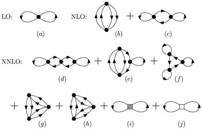
Figure 1: Hugenholtz diagrams for a dilute Fermi gas through next-to-next-to-leading-order (NNLO) in an EFT expansion.

The zeroth-order equation from Eq. (19) is

$${\widetilde{\Gamma}_{0}}[\rho,\tau]={\widetilde{W}_{0}}[J_{0},\eta_{0}]-\int\!d^{3}{\bf\bf{x}}\ J_{0}({\bf\bf{x}})\ \rho({\bf\bf{x}})-\int\!d^{3}{\bf\bf{x}}\ \eta_{0}({\bf\bf{x}})\ \tau({\bf\bf{x}})\ .$$ (21)

The corresponding zeroth order expansion of Eqs. (12) and (13) is

$$\rho({\bf\bf{x}})=\frac{\delta{\widetilde{W}}_{0}[J_{0},\eta_{0}]}{\delta J_{0}({\bf\bf{x}})}\ ,\qquad\tau({\bf\bf{x}})=\frac{\delta{\widetilde{W}}_{0}[J_{0},\eta_{0}]}{\delta\eta_{0}({\bf\bf{x}})}\ ,$$ (22)

(this also follows by taking functional derivatives of Eq. (21) with respect to $\rho$ and $\tau$ and using invertibility again, see PUG02 ). Note that these are the exact ground-state densities. Because $\rho$ and $\tau$ are treated as order unity, this is the only equation in the expansion of Eqs. (12) and (13) in which they appear. Thus, the sources $J_{0}({\bf\bf{x}})$ and $\eta_{0}({\bf\bf{x}})$ are particular functions that generate the expectation values $\rho$ and $\tau$ from the noninteracting system defined by $\lambda=0$. (The existence of $J_{0}({\bf\bf{x}})$ and $\eta_{0}({\bf\bf{x}})$ is the heart of the Kohn-Sham approach.) The inversion method achieves this end by construction.

The exponent in the non-interacting generating functional $Z_{0}[J,\eta]$ is quadratic in the fermion fields,

$$\int\!d^{4}x\ \psi^{\dagger}\biggl{[}i\partial_{t}+\frac{\nabla^{\,2}}{2M}-v({\bf\bf{x}})+J_{0}({\bf\bf{x}})\biggr{]}\psi+\int\!d^{4}x\ \eta_{0}({\bf\bf{x}})\nabla\psi^{\dagger}\cdot\nabla\psi$$ (23)

$$=\int\!d^{4}x\ \psi^{\dagger}\biggl{[}i\partial_{t}+\frac{\nabla^{\,2}}{2M}-v({\bf\bf{x}})+J_{0}({\bf\bf{x}})-\nabla\cdot\eta_{0}({\bf\bf{x}})\nabla\biggr{]}\psi\ ,$$

which leads us to define the Green’s function ${G}_{{\rm ks}}^{0}$ of the Kohn-Sham non-interacting system. This Green’s function satisfies

$$\left(i\partial_{t}+\nabla\cdot\frac{1}{2M^{*}({\bf\bf{x}})}\nabla-v({\bf\bf{x}})+J_{0}({\bf\bf{x}})\right){G}_{{\rm ks}}^{0}({\bf\bf{x}}t,{\bf\bf{x}}^{\prime}t^{\prime})=\delta^{3}({\bf\bf{x}}-{\bf\bf{x}}^{\prime})\delta(t-t^{\prime})$$ (24)

with finite density boundary conditions FETTER71 and a position-dependent effective mass defined by

$$\frac{1}{2M^{*}({\bf\bf{x}})}\equiv\frac{1}{2M}-\eta_{0}({\bf\bf{x}})\ .$$ (25)

Kohn-Sham orbitals arise as solutions to

$$\bigl{[}-\nabla\cdot\frac{1}{2M^{*}({\bf\bf{x}})}\nabla+v({\bf\bf{x}})-J_{0}({\bf\bf{x}})\bigr{]}\,\psi_{k}({\bf x})=\varepsilon_{k}\psi_{k}({\bf x})\,,$$ (26)

where the index $k$ represents all quantum numbers except for the spin. Note that Eq. (26) is in the form of the Skyrme single-particle equation [Eq. (7)] (without the spin-orbit part).

The spectral decomposition of ${G}_{{\rm ks}}^{0}$ in terms of the Kohn-Sham orbitals is PUG02

$$i{G}_{{\rm ks}}^{0}({\bf\bf{x}}t,{\bf\bf{x}}^{\prime}t^{\prime})=\sum_{k}\psi_{k}({\bf\bf{x}})\,\psi_{k}^{*}({\bf\bf{x}}^{\prime})\,e^{-i\varepsilon_{k}(t-t^{\prime})}[\theta(t-t^{\prime})\,\theta(\varepsilon_{k}-\varepsilon_{\rm F})-\theta(t^{\prime}-t)\,\theta(\varepsilon_{\rm F}-\varepsilon_{k})]\ .$$ (27)

It follows that ${\widetilde{W}}_{0}[J_{0},\eta_{0}]\propto{\rm Tr}\ln({G}_{{\rm ks}}^{0})^{-1}$ (since it is quadratic it yields a simple determinant), corresponding to the system without interactions, and can be written explicitly in terms of the single-particle Kohn-Sham eigenvalues as NEGELE88

$${\widetilde{W}}_{0}[J_{0},\eta_{0}]=-\nu\sum_{\varepsilon_{k}\leq\varepsilon_{\rm F}}\varepsilon_{k}\ ,$$ (28)

where $\nu$ is the spin-isospin degeneracy, as expected for a system without interactions. Equation (22) applied to Eq. (28) [with the help of Eq. (26)] implies that $\rho({\bf\bf{x}})$ and $\tau({\bf\bf{x}})$ follow as in Eq. (6) from the orbitals PUG02 . By using Eq. (28) in Eq. (21) and then eliminating $\varepsilon_{k}$ using Eq. (26), the lowest order effective action can be written two ways,

$${\widetilde{\Gamma}}_{0}[\rho,\tau] = -\nu\sum_{k}^{\rm occ.}\varepsilon_{k}-\int\!d^{3}{\bf\bf{x}}\ J_{0}({\bf\bf{x}})\ \rho({\bf\bf{x}})-\int\!d^{3}{\bf\bf{x}}\ \eta_{0}({\bf\bf{x}})\ \tau({\bf\bf{x}})$$ (29)

$$= -T_{s}[\tau]-\int\!d^{3}{\bf\bf{x}}\ v({\bf\bf{x}})\ \rho({\bf\bf{x}})\ ,$$

where

$$T_{s}[\tau]=\nu\sum_{k}\int\!d^{3}{\bf\bf{x}}\ \psi_{k}^{*}({\bf\bf{x}})\left(-{\nabla^{2}\over 2M}\right)\psi_{k}({\bf\bf{x}})={\nu\over 2M}\sum_{k}\int\!d^{3}{\bf\bf{x}}\ |\nabla\,\psi_{k}({\bf x})|^{2}={1\over 2M}\int\!d^{3}{\bf\bf{x}}\ \tau({\bf\bf{x}})$$ (30)

is the total kinetic energy of the KS non-interacting system.

The first-order equation in $\lambda$ from Eq. (19) is

$${\widetilde{\Gamma}}_{1}[\rho,\tau] = {\widetilde{W}}_{1}[J_{0},\eta_{0}]+\int\!d^{3}{\bf\bf{x}}\,\frac{\delta{\widetilde{W}}_{0}[J_{0},\eta_{0}]}{\delta J_{0}({\bf\bf{x}})}J_{1}({\bf\bf{x}})+\int\!d^{3}{\bf\bf{x}}\,\frac{\delta{\widetilde{W}}_{0}[J_{0},\eta_{0}]}{\delta\eta_{0}({\bf\bf{x}})}\eta_{1}({\bf\bf{x}})$$ (31)

$$\qquad\hbox{}-\int\!d^{3}{\bf\bf{x}}\ J_{1}({\bf\bf{x}})\ \rho({\bf\bf{x}})-\int\!d^{3}{\bf\bf{x}}\ \eta_{1}({\bf\bf{x}})\ \tau({\bf\bf{x}})$$

$$= {\widetilde{W}}_{1}[J_{0},\eta_{0}]\ .$$

The complete cancellation of the $J_{1}$ and $\eta_{1}$ terms from applying Eq. (22) occurs for the $J_{l}$ and $\eta_{l}$ terms in the equation for ${\widetilde{\Gamma}}_{l}$ for all $l\geq 1$. Thus for a given $l$, we only need ${\widetilde{W}}_{k}$’s with $k$ less than or equal to $l$, and $J_{k}$’s and $\eta_{k}$’s with $k$ smaller than $l$. The ${\widetilde{W}}_{k}$ functionals are constructed using conventional Feynman rules in position space with factors as in Ref. HAMMER00 , but with fermion lines representing $i{G}_{{\rm ks}}^{0}$.

In particular, the LO effective action is given by PUG02

$${\widetilde{\Gamma}}_{1}[\rho,\tau]={\widetilde{W}}_{1}[J_{0},\eta_{0}]={1\over 2}\,\nu\,(\nu-1)\,C_{0}\int d^{3}{\bf\bf{x}}\ {G}_{{\rm ks}}^{0}(x,x^{+})\,{G}_{{\rm ks}}^{0}(x,x^{+})\ .$$ (32)

The density can be directly expressed in terms of the Kohn-Sham Green’s function with equal arguments as

$$\rho({\bf\bf{x}})=-i\nu\,{G}_{{\rm ks}}^{0}(x,x^{+})\ ,$$ (33)

so that we have

$${\widetilde{\Gamma}}_{1}[\rho,\tau]=-{1\over 2}{(\nu-1)\over\nu}\ C_{0}\int d^{3}{\bf\bf{x}}\ |\rho({\bf\bf{x}})|^{2}\equiv{\widetilde{\Gamma}}_{1}[\rho]\ ,$$ (34)

which is minus the Hartree-Fock energy. Using Eq. (20), we obtain

$$J_{1}({\bf\bf{x}})={C_{0}\,(\nu-1)\over\nu}\ \rho({\bf\bf{x}})\ ,\qquad\quad\eta_{1}({\bf\bf{x}})=0\ .$$ (35)

After canceling the $J_{2}$ and $\eta_{2}$ terms as advertised above, the second-order effective action is given by

$${\widetilde{\Gamma}}_{2}[\rho,\tau] = {\widetilde{W}}_{2}[J_{0},\eta_{0}]+\int\!d^{3}{\bf\bf{x}}\,\frac{\delta{\widetilde{W}}_{1}[J_{0},\eta_{0}]}{\delta J_{0}({\bf\bf{x}})}J_{1}({\bf\bf{x}})+\int\!d^{3}{\bf\bf{x}}\,\frac{\delta{\widetilde{W}}_{1}[J_{0},\eta_{0}]}{\delta\eta_{0}({\bf\bf{x}})}\eta_{1}({\bf\bf{x}})$$ (36)

$$+ \frac{1}{2}\int\!d^{3}{\bf\bf{x}}\,d^{3}{\bf y}\,\frac{\delta^{2}{\widetilde{W}}_{0}[J_{0},\eta_{0}]}{\delta J_{0}({\bf\bf{x}})\,\delta J_{0}({\bf y})}J_{1}({\bf\bf{x}})\,J_{1}({\bf y})+\frac{1}{2}\int\!d^{3}{\bf\bf{x}}\,d^{3}{\bf y}\,\frac{\delta^{2}{\widetilde{W}}_{0}[J_{0},\eta_{0}]}{\delta\eta_{0}({\bf\bf{x}})\,\delta\eta_{0}({\bf y})}\eta_{1}({\bf\bf{x}})\,\eta_{1}({\bf y})$$

$$+ \int\!d^{3}{\bf\bf{x}}\,d^{3}{\bf y}\,\frac{\delta^{2}{\widetilde{W}}_{0}[J_{0},\eta_{0}]}{\delta J_{0}({\bf\bf{x}})\,\delta\eta_{0}({\bf y})}J_{1}({\bf\bf{x}})\,\eta_{1}({\bf y})\ .$$

${W}_{2}[J_{0},\eta_{0}]$ is calculated from the graphs Figs. 1(b) and (c):

$${W}_{2}[J_{0},\eta_{0}] = i\nu(\nu-1){C_{0}^{2}\over 4}\ \int\!d^{4}x\ d^{4}y\ {G}_{{\rm ks}}^{0}(x,y){G}_{{\rm ks}}^{0}(x,y){G}_{{\rm ks}}^{0}(y,x){G}_{{\rm ks}}^{0}(y,x)$$ (37)

$$\hskip 8.53581pt\hbox{}-i\nu(\nu-1)^{2}\ {C_{0}^{2}\over 2}\int\!d^{4}x\ d^{4}y\ {G}_{{\rm ks}}^{0}(x,x^{+}){G}_{{\rm ks}}^{0}(x,y){G}_{{\rm ks}}^{0}(y,x){G}_{{\rm ks}}^{0}(y,y^{+})\ .$$

The other terms in ${\widetilde{\Gamma}}_{2}$ completely cancel against the “anomalous” graph of Fig. 1(c) so that

$${\Gamma}_{2}[\rho,\tau]=i\nu(\nu-1)\,{C_{0}^{2}\over 4}\int\!d^{4}x\ d^{4}y\ {G}_{{\rm ks}}^{0}(x,y){G}_{{\rm ks}}^{0}(x,y){G}_{{\rm ks}}^{0}(y,x){G}_{{\rm ks}}^{0}(y,x)\,,$$ (38)

which is equal to the contribution made by the “beachball” diagram [Fig. 1(b)] to the energy [up to the time factor of Eq. (15)]. This cancellation is proven exactly as in Ref. PUG02 after generalizing to the matrix notation of Eq. (16). Calculation of the third-order effective action in the inversion method similarly leads to cancellation of the “anomalous” graphs in ${\widetilde{W}}_{3}$ given by Figs. 1(d), (e), and (f), leaving only Fig. 1(g) through (j) as contributors. All higher orders in ${\widetilde{\Gamma}}[\rho,\tau,\lambda]$ are determined in a similar manner, as described in Refs. VALIEV97 ; PUG02 .

In order to solve for the orbitals in Eq. (26) and to calculate the energy, we need expressions for $J_{0}({\bf\bf{x}})$ and $\eta_{0}({\bf\bf{x}})$. Since $J({\bf\bf{x}})=\eta({\bf\bf{x}})=0$ in the ground state, Eq. (17) becomes a variational principle that, together with Eq. (20), yields self-consistent expressions for $J_{0}$ and $\eta_{0}$ PUG02 :

$$J_{0}({\bf\bf{x}})\Bigr{|}_{{\rm gs}} = -\sum_{l\geq 1}J_{l}({\bf\bf{x}})\Bigr{|}_{{\rm gs}}=\left.\frac{\delta\widetilde{\Gamma}_{\rm int}[\rho,\tau]}{\delta\rho({\bf\bf{x}})}\right|_{{\rm gs}}\,,$$ (39)

$$\eta_{0}({\bf\bf{x}})\Bigr{|}_{{\rm gs}} = -\sum_{l\geq 1}\eta_{l}({\bf\bf{x}})\Bigr{|}_{{\rm gs}}=\left.\frac{\delta\widetilde{\Gamma}_{\rm int}[\rho,\tau]}{\delta\tau({\bf\bf{x}})}\right|_{{\rm gs}}\ ,$$ (40)

where $\widetilde{\Gamma}_{\rm int}[\rho,\tau]$ is the interaction effective action

$$\widetilde{\Gamma}_{\rm int}[\rho,\tau]\equiv\sum_{l\geq 1}{\widetilde{\Gamma}}_{l}[\rho,\tau]\ ,$$ (41)

and the subscript “$\rm gs$” refers to the ground-state. (Note that at this stage $\lambda=1$, and Eqs. (39) and (40) mix all orders of the original inversion-method expansion into the Kohn-Sham potentials $J_{0}$ and $\eta_{0}$.) A given approximation corresponds to truncating Eq. (41) at $l_{\rm max}$ and then carrying out the self-consistent calculation. We refer to $l_{\rm max}=1$ as leading order, or LO, $l_{\rm max}=2$ as next-to-leading order or NLO, and $l_{\rm max}=3$ as NNLO.

II.2 EFT for Dilute Fermi Systems

The non-interacting energy density at zero temperature for $A$ particles with spin-degeneracy $\nu$ in volume $V$ can be written as

$${\cal E}_{0}={3\over 5}\left({k_{\rm F}^{2}\over 2M}\right)\rho\ ,$$ (42)

where the density $\rho$ is

$$\rho=\frac{A}{V}=\nu\int{d^{3}k\over(2\pi)^{3}}\ \theta(k_{\rm F}-k)={\nu k_{F}^{3}\over 6\pi^{2}}\ .$$ (43)

For a uniform system, the order-by-order in $k_{\rm F}a_{s}$ corrections to Eq. (42) due to interactions can be calculated in the EFT via the Hugenholtz diagrams in Fig. 1, as described in Ref. HAMMER00 .

For a dilute Fermi system, the coefficients $C_{0}$, $C_{2}$, and $C_{2}^{\prime}$ can be expressed in terms of the effective-range parameters by matching to the effective-range expansion for low-energy fermion-fermion scattering HAMMER00 :

$$C_{0}=\frac{4\pi a_{s}}{M},\qquad C_{2}=C_{0}\frac{a_{s}r_{s}}{2},\quad\mbox{and}\quad C_{2}^{\prime}=\frac{4\pi a_{p}^{3}}{M}\,,$$ (44)

where $a_{s}$ ($a_{p}$) is the $s$-wave ($p$-wave) scattering length and $r_{s}$ is the $s$-wave effective range, respectively. If the effective range parameters are all of order the interaction range, then the EFT is said to be natural. In a uniform system at finite density, the mean inter-particle spacing $r_{0}$ provides a length scale for comparison; the ratio $a_{s}/r_{0}\sim k_{F}a_{s}$ provides a dimensionless measure of density, where $k_{F}$ is the Fermi momentum. In the dilute regime, $k_{F}a_{s}\ll 1$ serves as an expansion parameter, as realized by the EFT of Ref. HAMMER00 where the diagrams of Fig. 1 each contributed to precisely one order in the energy density: LO or ${\cal E}_{1}$ is ${\cal O}(k_{\rm F}^{6})$, NLO or ${\cal E}_{2}$ is ${\cal O}(k_{\rm F}^{7})$, and NNLO or ${\cal E}_{3}$ is ${\cal O}(k_{\rm F}^{8})$.

In extending these results to a finite system, the simplest approximation that can be invoked is the local density approximation (LDA). In Ref. PUG02 , the results for a uniform system were used in the LDA to evaluate the ${\widetilde{\Gamma}}_{l}$ and hence the energy through NNLO. We simply quote the results here. The LO diagram [Fig. 1(a)] is the Hartree-Fock contribution, which is purely local. Thus, it is an exact evaluation and Eq. (34) can be used directly for the energy contribution:

$$E_{HF}[\rho({\bf\bf{x}})]=\int\!d^{3}{\bf\bf{x}}\ {\cal E}_{1}[\rho({\bf\bf{x}})]={1\over 2}{(\nu-1)\over\nu}\ C_{0}\int d^{3}{\bf\bf{x}}\ |\rho({\bf\bf{x}})|^{2}\ .$$ (45)

The contributions to the energy from NLO and NNLO diagrams are computed in LDA by simply integrating the corresponding uniform energy densities evaluated at the local density PUG02 :

$$E^{\rm LDA}_{c}[\rho({\bf\bf{x}})] = \int\!d^{3}{\bf\bf{x}}\,\left\{{\cal E}_{2}(\rho_{0})+{\cal E}_{3}(\rho_{0})\right\}\,|_{\rho_{0}\rightarrow\rho({\bf\bf{x}})}$$ (46)

$$= b_{1}\,{a_{s}^{2}\over 2M}\int\!d^{3}{\bf\bf{x}}\,[\rho({\bf\bf{x}})]^{7/3}$$

$$\hbox{}+\left(b_{2}\,a_{s}^{2}\,r_{s}+b_{3}\,a_{p}^{3}+b_{4}\,a_{s}^{3}\right){1\over 2M}\int\!d^{3}{\bf\bf{x}}\,[\rho({\bf\bf{x}})]^{8/3}\ ,$$

where the dimensionless $b_{k}$ are

$$b_{1} = {4\over 35\pi^{2}}\,(\nu-1)\left({6\pi^{2}\over\nu}\right)^{4/3}\,(11-2\ln 2)\ ,$$

$$b_{2} = {1\over 10\pi}\,(\nu-1)\left({6\pi^{2}\over\nu}\right)^{5/3}\ ,$$

$$b_{3} = {1\over 5\pi}\,(\nu+1)\left({6\pi^{2}\over\nu}\right)^{5/3}\ ,$$

$$b_{4} = \left({6\pi^{2}\over\nu}\right)^{5/3}\biggl{(}0.0755\,(\nu-1)+0.0574\,(\nu-1)(\nu-3)\biggr{)}\ .$$ (47)

The numerical constants in the last line of Eq. (47) were obtained by Monte Carlo integration HAMMER00 .

II.3 Including $\tau$ in Hartree-Fock Diagrams

The contributions to $E^{\rm LDA}_{c}[\rho({\bf\bf{x}})]$ from the Hartree-Fock graphs containing the $C_{2}$ and $C^{\prime}_{2}$ vertices [Figs. 1(i) and (j)], which have gradients, were approximately evaluated in the LDA in Eq. (46) to obtain a functional of $\rho$ alone. In the DFT formalism generalized to include the kinetic energy density $\tau({\bf\bf{x}})$, however, we observe that they can be evaluated exactly in terms of $\rho({\bf\bf{x}})$ and $\tau({\bf\bf{x}})$ (for closed shells). These contributions to ${\widetilde{W}}_{3}[J_{0},\eta_{0}]$ can be simply expressed in terms of gradients acting on the Kohn-Sham Green’s functions [cf. Eq. (32)]:

$${\widetilde{W}}_{3}[J_{0},\eta_{0}] = -{1\over 16}\int d^{3}{\bf\bf{x}}\ \biggl{[}C_{2}\,\nu\,(\nu-1)\,\left\{(\bm{\nabla}_{1}-\bm{\nabla}_{2})^{2}+(\bm{\nabla}_{3}-\bm{\nabla}_{4})^{2}\right\}$$ (48)

$$\qquad\qquad\qquad\hbox{}+2C^{\prime}_{2}\,\nu\,(\nu+1)\,\left\{(\bm{\nabla}_{1}-\bm{\nabla}_{2})\cdot(\bm{\nabla}_{3}-\bm{\nabla}_{4})\right\}\biggr{]}$$

$$\qquad\qquad\qquad\qquad{G}_{{\rm ks}}^{0}(x_{4},x_{2}^{+})\,{G}_{{\rm ks}}^{0}(x_{3},x_{1}^{+})\biggr{|}_{x_{1}=x_{2}=x_{3}=x_{4}=x}\ +\cdots$$

Equation (48) is evaluated by carrying out the gradients and then setting all of the $x_{i}$ equal to $x$. For this purpose, the replacement

$${G}_{{\rm ks}}^{0}(x,x^{\prime})\longrightarrow i\sum_{k}^{\rm occ.}\psi_{k}({\bf\bf{x}})\psi^{*}_{k}({\bf\bf{x}}^{\prime})$$ (49)

can be made and, since in the end we integrate over ${\bf\bf{x}}$, we can partially integrate any term. It is not difficult to write the resulting expressions in terms of $\rho({\bf\bf{x}})$, $\tau({\bf\bf{x}})$, and a current density $\bm{j}({\bf\bf{x}})$,

$$\bm{j}({\bf\bf{x}})=\frac{i}{2}\nu\sum_{k}^{\rm occ.}\left[\bm{\nabla}\psi^{*}_{k}({\bf\bf{x}})\psi_{k}({\bf\bf{x}})-\psi^{*}_{k}({\bf\bf{x}})\bm{\nabla}\psi_{k}({\bf\bf{x}})\right]\ .$$ (50)

The current density vanishes when summed over closed shells, leaving simple expressions for the Hartree-Fock energy functionals:

$$E_{C_{2}}[\rho({\bf\bf{x}}),\tau({\bf\bf{x}})]={B_{2}\,a_{s}^{2}\,r_{s}\over 2M}\int\!d^{3}{\bf\bf{x}}\,[\rho({\bf\bf{x}})\tau({\bf\bf{x}})+\frac{3}{4}\left(\bm{\nabla}\rho\right)^{2}]\ ,$$ (51)

$$E_{C^{{}^{\prime}}_{2}}[\rho({\bf\bf{x}}),\tau({\bf\bf{x}})]={B_{3}\,a_{p}^{3}\over 2M}\int\!d^{3}{\bf\bf{x}}\,[\rho({\bf\bf{x}})\tau({\bf\bf{x}})-\frac{1}{4}\left(\bm{\nabla}\rho\right)^{2}]\ .$$ (52)

The dimensionless constants $B_{2}$ and $B_{3}$ are given by

$$B_{2}=\pi\,{(\nu-1)\over\nu}\ ,\qquad B_{3}=2\,\pi\,{(\nu+1)\over\nu}\ .$$ (53)

The total contribution to the energy from NLO and NNLO diagrams is

$$E_{c}[\rho({\bf\bf{x}}),\tau({\bf\bf{x}})] = {b_{1}\,a_{s}^{2}\over 2M}\int\!d^{3}{\bf\bf{x}}\,[\rho({\bf\bf{x}})]^{7/3}+E_{C_{2}}[\rho({\bf\bf{x}}),\tau({\bf\bf{x}})]$$ (54)

$$+\,E_{C^{{}^{\prime}}_{2}}[\rho({\bf\bf{x}}),\tau({\bf\bf{x}})]+\,{b_{4}\,a_{s}^{3}\over 2M}\int\!d^{3}{\bf\bf{x}}\,[\rho({\bf\bf{x}})]^{8/3}\ .$$

Since this functional now has the semi-local $\tau({\bf\bf{x}})$ as one of its ingredients, it represents a step beyond LDA, even though the contributions from Figs. 1(b), (g), and (h) are still evaluated with the LDA prescription. The next step in the DFT/EFT program will be to develop systematic expansions to these contributions in terms of $\rho$ and $\tau$.

For now, we carry out the DFT/EFT formalism in the effective action framework using the hybrid functional with $\tau({\bf\bf{x}})$. The full effective action is given by

$${\widetilde{\Gamma}}[\rho,\tau]={\widetilde{\Gamma}}_{0}[\rho,\tau]+{\widetilde{\Gamma}}_{1}[\rho,\tau]+\sum_{k=2}^{\infty}\,{\widetilde{\Gamma}}_{k}[\rho,\tau]\ .$$ (55)

We proceed to calculate the sources using Eqs. (39), (40), and (54) to NNLO; first $J_{0}({\bf\bf{x}})$ is

$$J_{0}({\bf\bf{x}}) = \frac{\delta}{\delta\rho({\bf\bf{x}})}\left({\widetilde{\Gamma}}_{1}[\rho,\tau]+\sum_{k=2}^{3}{\widetilde{\Gamma}}_{k}[\rho,\tau]\right)=-{\delta\over\delta\rho({\bf\bf{x}})}\left(E_{\rm HF}[\rho]+E_{c}[\rho,\tau]\right)$$ (56)

$$= -\frac{(\nu-1)}{\nu}\,\frac{4\pi\,a_{s}}{M}\,\rho({\bf\bf{x}})-{7\over 3}\,b_{1}\,\frac{a_{s}^{2}}{2M}\,[\rho({\bf\bf{x}})]^{4/3}-\frac{8}{3}\,b_{4}\,\frac{a_{s}^{3}}{2M}[\rho({\bf\bf{x}})]^{5/3}$$

$$-\left(B_{2}\,a_{s}^{2}\,r_{s}+B_{3}\,a_{p}^{3}\right)\frac{1}{2M}\,\tau({\bf\bf{x}})+\left(3B_{2}\,a_{s}^{2}\,r_{s}-B_{3}\,a_{p}^{3}\right)\frac{1}{4M}\,{\nabla}^{2}\rho({\bf\bf{x}})\ ,$$

and then $\eta_{0}({\bf\bf{x}})$ is:

$$\eta_{0}({\bf\bf{x}})=-{\delta\over\delta\tau({\bf\bf{x}})}\left(E_{\rm HF}[\rho]+E_{c}[\rho,\tau]\right)=-\left(B_{2}\,a_{s}^{2}\,r_{s}+B_{3}\,a_{p}^{3}\right)\frac{1}{2M}\,\rho({\bf\bf{x}})\ .$$ (57)

The spatially dependent effective mass $M^{*}({\bf\bf{x}})$ is therefore

$$\frac{1}{2M^{*}({\bf\bf{x}})}=\frac{1}{2M}-\eta_{0}({\bf\bf{x}})=\frac{1}{2M}+\left[{(\nu-1)\over{4\nu}}\,C_{2}+{(\nu+1)\over{4\nu}}\,C^{\prime}_{2}\right]\,\rho({\bf\bf{x}})\ ,$$ (58)

where Eq. (44) has been used. An expression for the total binding energy (through NNLO) follows by substituting for $J_{0}({\bf\bf{x}})$ and $\eta_{0}({\bf\bf{x}})$ in Eq. (29) and then using Eq. (55) and Eq. (15),

$$E[\rho({\bf\bf{x}}),\tau({\bf\bf{x}})] = \nu\sum_{k}^{\rm occ.}\varepsilon_{k}-\int\!d^{3}{\bf\bf{x}}\,\biggl{\{}\frac{1}{2}\frac{(\nu-1)}{\nu}\,\frac{4\pi\,a_{s}}{M}\,[\rho({\bf\bf{x}})]^{2}+\frac{4}{3}\,b_{1}\,\frac{a_{s}^{2}}{2M}\,[\rho({\bf\bf{x}})]^{7/3}$$ (59)

$$+ \hbox{}\frac{5}{3}\,b_{4}\,\frac{a_{s}^{3}}{2M}\,[\rho({\bf\bf{x}})]^{8/3}+\left(3B_{2}\,a_{s}^{2}\,r_{s}-B_{3}\,a_{p}^{3}\right)\frac{1}{8M}\,{[\nabla\rho({\bf\bf{x}})]}^{2}$$

$$+ \hbox{}\left(B_{2}\,a_{s}^{2}\,r_{s}+B_{3}\,a_{p}^{3}\right)\frac{1}{2M}\,\rho({\bf\bf{x}})\tau({\bf\bf{x}})\biggr{\}}\ .$$

The noninteracting case ($C_{i}\equiv 0$) uses $J_{0}({\bf\bf{x}})\equiv 0$, $\eta_{0}({\bf\bf{x}})\equiv 0$ and the first term in Eq. (59). Leading order (LO) uses the first term in Eq. (56) and the first two terms in Eq. (59), and so on for NLO and NNLO. An alternative expression for the energy is obtained by using the second part of Eq. (29) followed by Eqs. (30), (55), and (15):

$$E[\rho({\bf\bf{x}}),\tau({\bf\bf{x}})] = \int\!d^{3}{\bf\bf{x}}\,\biggl{\{}{1\over 2M}\tau({\bf\bf{x}})+\,v({\bf\bf{x}})\,\rho({\bf\bf{x}})+\frac{1}{2}\frac{(\nu-1)}{\nu}\,\frac{4\pi\,a_{s}}{M}\,[\rho({\bf\bf{x}})]^{2}$$ (60)

$$+ \left(B_{2}\,a_{s}^{2}\,r_{s}+B_{3}\,a_{p}^{3}\right)\frac{1}{2M}\,\rho({\bf\bf{x}})\,\tau({\bf\bf{x}})+\left(3B_{2}\,a_{s}^{2}\,r_{s}-B_{3}\,a_{p}^{3}\right)\frac{1}{8M}\,{[\nabla\rho({\bf\bf{x}})]}^{2}$$

$$+ b_{1}\,\frac{a_{s}^{2}}{2M}\,[\rho({\bf\bf{x}})]^{7/3}+b_{4}\,\frac{a_{s}^{3}}{2M}\,[\rho({\bf\bf{x}})]^{8/3}\biggr{\}}\ .$$

II.4 Comparison to Skyrme Hartree-Fock

A nucleus is a self-bound system, so the external potential $v({\bf\bf{x}})=0$. To compare the DFT/EFT functional to the conventional Skyrme energy density functional of Eq. (5), we set the spin multiplicity $\nu=4$ and use Eq. (44) to rewrite Eq. (60) in terms of the $C_{i}$’s, obtaining the energy density:

$${\cal E}[\rho({\bf\bf{x}}),\tau({\bf\bf{x}})]={1\over 2M}\tau({\bf\bf{x}}) + \frac{3}{8}C_{0}\,[\rho({\bf\bf{x}})]^{2}+\frac{1}{16}(3C_{2}+5C^{{}^{\prime}}_{2})\rho{({\bf\bf{x}})}\,\tau{({\bf\bf{x}})}+\frac{1}{64}(9C_{2}-5C^{{}^{\prime}}_{2})(\bm{\nabla}\rho)^{2}$$ (61)

$$+ b_{1}\,\frac{a_{s}^{2}}{2M}[\rho({\bf\bf{x}})]^{7/3}+b_{4}\,\frac{a_{s}^{3}}{2M}[\rho({\bf\bf{x}})]^{8/3}\ .$$

We observe that we get all the terms of ${\cal E}_{SK}({\bf\bf{x}})$ from Eq. (5) except for the one with coefficient $t_{3}$ and the spin-dependent terms, if we make the correspondence $t_{0}\leftrightarrow C_{0}$, $t_{1}\leftrightarrow C_{2}$ and $t_{2}\leftrightarrow C^{{}^{\prime}}_{2}$. This correspondence is not surprising since the Skyrme interaction was originally motivated as a low-momentum expansion of the G matrix SKYRME . The two additional terms in Eq. (61) of the form ${\rho({\bf\bf{x}})}^{2+\alpha}$ come from correlations (i.e., terms beyond Hartree-Fock), but there is no direct association with the $t_{3}$ term in the Skyrme energy density, which was originally motivated as a three-body contribution (so $\alpha=1$). However, it is clear that the Skyrme functional is incomplete as an expansion; a direct connection to microscopic interactions by matching to an EFT will include at least these additional terms.

The generalization of the DFT/EFT to include spin and isospin dependence is straightforward. If one writes a complete set of four-fermion terms with $\bm{\sigma}$ and $\bm{\tau}$ matrices in the EFT Lagrangian, there are redundant terms because of Fermi statistics. In conventional discussions of the Skyrme approach, this observation is typically cast in terms of antisymmetrization of the interaction VB72 ; RINGSCHUCK . For a path integral formulation of the DFT/EFT, using Fierz rearrangement is a convenient alternative. We illustrate the procedure for the leading spin dependence.

First consider just spin-1/2 (no isospin, so $\nu=2$). We expand the product of Grassmann fields $\psi_{i}\psi^{\dagger}_{j}$ ($i$ and $j$ are spin indices) in the complete basis of $\delta_{ij}$ and $\sigma^{a}_{ij}$ ($a=\{1,2,3\}$), identifying the coefficients by contracting in turn with $\delta_{ij}$ and $\sigma^{b}_{ji}$. The result, with minus signs from interchanging Grassmann fields, is

$$\psi_{i}\psi^{\dagger}_{j}=-\frac{1}{2}(\psi^{\dagger}\psi)\delta_{ij}-\frac{1}{2}(\psi^{\dagger}\sigma^{a}\psi)\sigma^{a}_{ij}\ .$$ (62)

If we substitute this result into $(\psi^{\dagger}\psi)^{2}=\psi^{\dagger}_{i}\{\psi_{i}\psi^{\dagger}_{j}\}\psi_{j}$, we find

$$(\psi^{\dagger}\psi)^{2}=-\frac{1}{2}(\psi^{\dagger}\psi)^{2}-\frac{1}{2}(\psi^{\dagger}\bm{\sigma}\psi)^{2}\ ,$$ (63)

or

$$(\psi^{\dagger}\bm{\sigma}\psi)^{2}=-3(\psi^{\dagger}\psi)^{2}\ .$$ (64)

(We could also start with $(\psi^{\dagger}_{i}\sigma^{a}_{ii^{\prime}}\psi_{i^{\prime}})(\psi^{\dagger}_{j}\sigma^{a}_{jj^{\prime}}\psi_{j^{\prime}})$ and obtain the same result with a bit more effort). Therefore

$$C_{0}(\psi^{\dagger}\psi)^{2}+C_{0}^{\sigma}(\psi^{\dagger}\bm{\sigma}\psi)^{2}=(C_{0}-3C_{0}^{\sigma})(\psi^{\dagger}\psi)^{2}$$ (65)

and the single term ${\widetilde{C}}_{0}(\psi^{\dagger}\psi)^{2}$ with ${\widetilde{C}}_{0}\equiv C_{0}-3C_{0}^{\sigma}$ yields the same results for all diagrams as the original two terms.

For the $\nu=4$ case with spin and isospin, we perform a similar procedure to find

$$\psi_{i\alpha}\psi^{\dagger}_{j\beta}=-\frac{1}{4}(\psi^{\dagger}\psi)\delta_{ij}\delta_{\alpha\beta}-\frac{1}{4}(\psi^{\dagger}\sigma^{a}\psi)\sigma^{a}_{ij}\delta_{\alpha\beta}-\frac{1}{4}(\psi^{\dagger}\tau^{b}\psi)\delta_{ij}\tau^{b}_{\alpha\beta}-\frac{1}{4}(\psi^{\dagger}\sigma^{a}\tau^{b}\psi)\sigma^{a}_{ij}\tau^{b}_{\alpha\beta}\ .$$ (66)

Substituting into any two of $(\psi^{\dagger}\psi)^{2}$, $(\psi^{\dagger}\bm{\sigma}\psi)^{2}$, $(\psi^{\dagger}\bm{\tau}\psi)^{2}$, and $(\psi^{\dagger}\bm{\sigma}\bm{\tau}\psi)^{2}$, we find two independent relations, which can be solved simultaneously to find:

$$(\psi^{\dagger}\bm{\tau}\psi)^{2} = -2(\psi^{\dagger}\psi)^{2}-(\psi^{\dagger}\bm{\sigma}\psi)^{2}$$ (67)

$$(\psi^{\dagger}\bm{\sigma}\bm{\tau}\psi)^{2} = -3(\psi^{\dagger}\psi)^{2}\ ,$$ (68)

which allow us to eliminate explicit dependence on $\bm{\tau}$ matrices in favor of just two independent couplings:

$$C_{0}(\psi^{\dagger}\psi)^{2}+C_{0}^{\sigma}(\psi^{\dagger}\bm{\sigma}\psi)^{2}+C_{0}^{\tau}(\psi^{\dagger}\bm{\tau}\psi)^{2}+C_{0}^{\sigma\tau}(\psi^{\dagger}\bm{\sigma}\bm{\tau}\psi)^{2}$$

$$\qquad\qquad=(C_{0}-2C_{0}^{\tau}-3C_{0}^{\sigma\tau})(\psi^{\dagger}\psi)^{2}+(C_{0}^{\sigma}-C_{0}^{\tau})(\psi^{\dagger}\bm{\sigma}\psi)^{2}\ .$$ (69)

This agrees (of course) with the usual discussion in terms of antisymmetrized interactions (e.g., see RINGSCHUCK or VB72 ). The choice to eliminate the $\bm{\tau}$ terms is purely conventional. The convention with Skyrme interactions is to choose the independent couplings to be $t_{i}$ and $x_{i}$, which multiply terms in the effective interaction in the combination $t_{i}(1+x_{i}P_{\sigma})$, with $P_{\sigma}$ the spin exchange operator. Extending to more derivatives and the spin-orbit (and tensor) terms follows systematically in the EFT approach, but introduces many more constants; complete sets of contact terms with more derivatives in the EFT Lagrangian can be found in Refs. VANKOLCK and EPELBAUM . The proliferation of constants leads to a clash of philosophies between the minimalist, phenomenological approach (use as few terms as possible), which is necessarily model dependent, and the model-independent EFT approach (use a complete set of terms).

The similarities of the successful Skyrme functional and the DFT functional for a dilute Fermi gas prompts an analysis of typical Skyrme parameters as effective range parameters. One can use the association of the $t_{i}$’s and the $C_{i}$’s along with numerical values from successful Skyrme parameterizations (e.g., Ref. BROWN98 ) to estimate “equivalent” values of $a_{s}$, $r_{s}$, and $a_{p}$. We find that $a_{s}\approx-2\mbox{--}3\,\mbox{fm}$, which is about the inverse pion mass and is much smaller than the large, fine-tuned values of the free-space nucleon-nucleon interaction (however, some Skyrme parameterization have an “equivalent” $a_{s}$ of $5\,\mbox{fm}$ or larger). However, $k_{\rm F}a_{s}$ is still significantly larger than unity inside a nucleus, which precludes a perturbative dilute expansion. Interestingly, the equivalent $r_{s}$ and $a_{p}$ values have magnitudes consistent with what one might expect from the nuclear hard-core radius (with $a_{p}<0$), leading to $k_{\rm F}r_{s}$ and $k_{\rm F}a_{p}$ less than unity.

III Results for Dilute Fermi System in a Trap

In this section, we present numerical results for the dilute Fermi system comprised of a small number of fermions confined in a harmonic oscillator trap. We compare the nature of the convergence of the EFT in a finite system both qualitatively and quantitatively to the analysis done purely in the LDA PUG02 , which means the effect of treating the Hartree-Fock contributions at NNLO [Fig. 1(i) and (j)] exactly.

III.1 Kohn-Sham Self-Consistent Procedure

We restrict our calculations to finding the Kohn-Sham orbitals for closed shells, so the density and potentials are functions only of the radial coordinate $r\equiv|{\bf\bf{x}}|$. Note that the basic procedure is the same one used for closed-shell nuclei in Skyrme-Hartree-Fock RINGSCHUCK , even though the DFT/EFT can include correlations to any order. The Kohn-Sham iteration procedure is as follows:

1. Start by solving the Schrödinger equation with the external potential profile $v(r)$ for the lowest $A$ states (including degeneracies) to find a set of orbitals and Kohn-Sham eigenvalues $\{\psi_{k},\varepsilon_{k}\}$.

2. Compute the density and kinetic energy density from the orbitals:

   $$\rho(r)=\sum_{k=1}^{A}|\psi_{k}({\bf x})|^{2}\ ,$$ (70)

   $$\tau(r)=\frac{1}{4\pi}\int\!d\Omega\,\tau({\bf\bf{x}})=\frac{1}{4\pi}\sum_{k=1}^{A}\int\!d\Omega\,|\nabla\,\psi_{k}({\bf x})|^{2}\ .$$ (71)

3. Using Eqs. (56)–(57), find $J_{0}(r)$ and $\eta_{0}(r)$. Evaluate the local single-particle potential

   $$v_{s}[\rho(r),\tau(r)]\equiv v_{s}(r)\equiv v(r)-J_{0}(r)$$ (72)

   at the chosen level of approximation (e.g., NLO) and the “effective” mass :

   $$\frac{1}{2M^{*}(r)}=\frac{1}{2M}-\eta_{0}(r)\ .$$ (73)

4. Solve the Skyrme-type Schrödinger equation for the lowest $A$ states (including degeneracies), to find $\{\psi_{k},\varepsilon_{k}\}$ as before:

   $$\bigl{[}-\nabla\frac{1}{2M^{*}(r)}\nabla+v_{s}(r)\bigr{]}\,\psi_{k}({\bf x})=\varepsilon_{k}\psi_{k}({\bf x})\,.$$ (74)

5. Repeat steps 2.–4. until changes are acceptably small (“self-consistency”). In practice, the changes in the density are “damped” by using a weighted average of the densities from the $(n-1)$th and $n$th iterations:

   $$\rho(r)=\beta\rho_{n-1}(r)+(1-\beta)\rho_{n}(r)\ ,$$ (75)

   with $0<\beta\leq 1$.

This procedure has been implemented for dilute fermions in a trap using two different methods for carrying out step 4. The Kohn-Sham single-particle equations are solved in one approach by direct integration of the differential equations and in the other approach by diagonalization of the single-particle Hamiltonian in a truncated basis of unperturbed harmonic oscillator wavefunctions. The same results are obtained to high accuracy. [Note that other methods used for Skyrme-type equations, such as the conjugate-gradient method REINHARD , can also be directly applied.]

III.2 Fermions in a Harmonic Trap

The interaction through NNLO is specified in terms of the three effective range parameters $a_{s}$, $r_{s}$, and $a_{p}$. For the numerical calculations presented here, we consider the natural case of hard-sphere repulsion with radius $R$, in which case $a_{s}=a_{p}=R$ and $r_{s}=2R/3$, and also the case with $a_{p}=2a_{s}$, so we can emphasize the effect of $M^{*}(r)/M$ significantly less than unity.

Lengths are measured in units of the oscillator parameter $b\equiv\sqrt{\hbar/M\omega}$, masses in terms of the fermion mass $M$, and $\hbar=1$. In these units, $\hbar\omega$ for the oscillator is unity and the Fermi energy of a non-interacting gas with filled shells up to $N_{F}$ is $E_{F}=(N_{F}+3/2)$. The total number of fermions $A$ is related to $N_{F}$ by

$$A=\frac{\nu}{6}(N_{F}+1)(N_{F}+2)(N_{F}+3)\ .$$ (76)

Since we have only considered spin-independent interactions, our results are independent of whether the spin degeneracy $\nu$ actually originates from spin, isospin, or some flavor index.

With interactions included, single-particle states are labeled by a radial quantum number $n$, an orbital angular momentum $l$ with $z$-component $m_{l}$, and the spin projection. The radial functions depend only on $n$ and $l$, so the degeneracy of each level is $\nu\times(2l+1)$. The solutions take the form (times a spinor, which is suppressed)

$$\psi_{nlm_{l}}({\bf\bf{x}})=R_{nl}(r)\,Y_{lm_{l}}(\Omega)=\frac{u_{nl}(r)}{r}\,Y_{lm_{l}}(\Omega)\ ,$$ (77)

where the radial function $u_{nl}(r)$ satisfies

$$\left[-\frac{1}{2M^{\ast}(r)}\frac{d^{2}}{dr^{2}}-\frac{d\eta_{0}}{dr}\,\left(\frac{1}{r}-\frac{d}{dr}\right)+v_{s}(r)+\frac{l(l+1)}{2M^{\ast}(r)r^{2}}\right]u_{nl}(r)=\varepsilon_{nl}u_{nl}(r)\ ,$$ (78)

and the $u_{nl}$’s are normalized according to

$$\int_{0}^{\infty}\!|u_{nl}(r)|^{2}\,dr=1\ .$$ (79)

Thus the density is given by

$$\rho(r)=\nu\,\sum_{nl}^{\rm occ.}\,\frac{(2l+1)}{4\pi}\,|R_{nl}(r)|^{2}\ ,$$ (80)

and the kinetic energy density is given by REINHARD

$$\tau(r)=\frac{\nu}{4\pi}\,\sum_{nl}^{\rm occ.}\,(2l+1)\left[{\left(\frac{dR_{nl}}{dr}\right)}^{2}+\frac{l(l+1)}{r^{2}}\,|R_{nl}(r)|^{2}\right]\ .$$ (81)

The interactions are sufficiently weak that the occupied states are in one-to-one correspondence with those occupied in the non-interacting harmonic oscillator potential.

III.3 Numerical Results

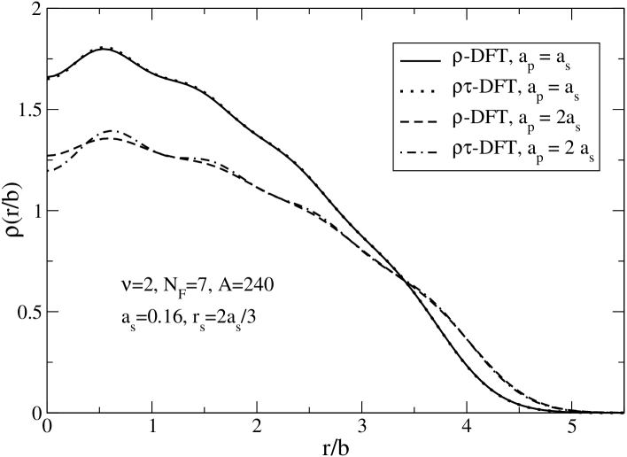
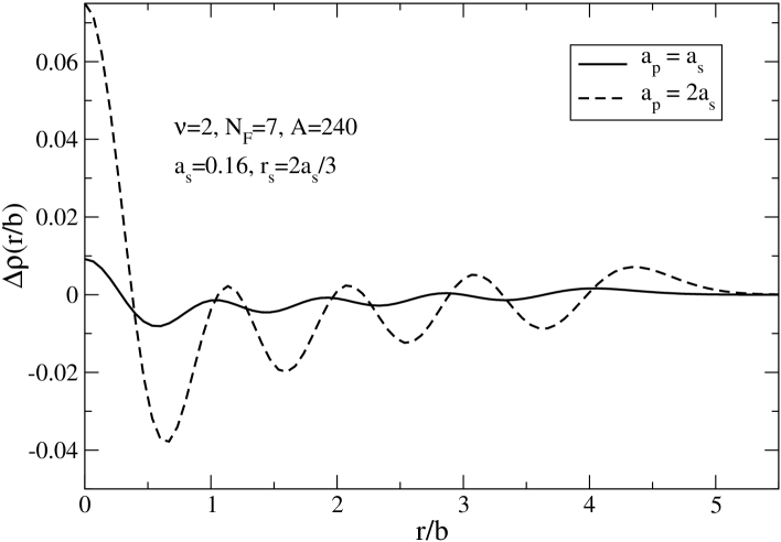
Figure 2: NNLO Kohn-Sham density distributions for a dilute gas of fermions in a harmonic trap with degeneracy $\nu=2$ filled up to $N_{\rm F}=7$, which implies there are 240 particles in the trap. The scattering length is $a_{s}=0.16$ and the effective range is $r_{s}=2a_{s}/3$. Results for two values of $a_{p}$ are compared for the LDA $\rho$-only functional ($\rho$–DFT) and with $\tau$ ($\rho\tau$–DFT).

Figure 3: Deviation of $\rho\tau$–DFT from $\rho$–DFT results at NNLO for the same systems as in Fig. 3.

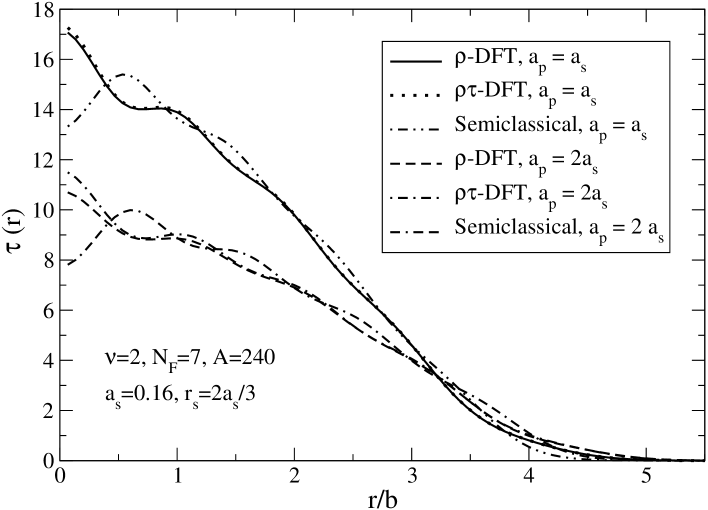
Figure 4: NNLO Kohn-Sham kinetic-energy-density distributions for the same systems as in Fig. 3. The upper three curves are for $a_{p}=a_{s}$ and the lower three curves are for $a_{p}=2a_{s}$.

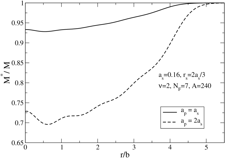
Figure 5: NNLO Kohn-Sham effective mass distributions for the same systems as in Fig. 3. Results for two values of $a_{p}$ are shown.

Table 1: Energies per particle, averages of the local Fermi momentum $k_{\rm F}$, and rms radii for sample parameters and particle numbers for a dilute Fermi gas in a harmonic trap. See the text for a description of units. The scattering length is fixed at $a_{s}=0.16$ and the effective range is set to $r_{s}=2a_{s}/3$ when $a_{p}\neq 0$. Results with the DFT functional including $\tau$ are marked “$\tau$–NNLO.”

$\nu$	$N_{F}$	$A$	$a_{p}$	$E/A$	$\langle k_{\rm F}\rangle$	$\sqrt{\langle r^{2}\rangle}$	approximation
2	7	240	–	$7.36$	3.08	$2.76$	LO
2	7	240	–	$7.51$	3.03	$2.81$	NLO (LDA)
2	7	240	0.00	$7.52$	3.02	$2.82$	NNLO (LDA)
2	7	240	0.16	$7.66$	2.97	$2.87$	NNLO (LDA)
2	7	240	0.16	$7.65$	2.97	$2.87$	$\tau$–NNLO (LDA)
2	7	240	0.32	$8.33$	2.76	$3.10$	NNLO (LDA)
2	7	240	0.32	$8.30$	2.77	$3.09$	$\tau$–NNLO (LDA)

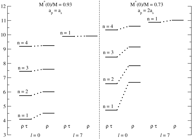
Figure 6: Comparison of selected single-particle energy spectra for the same systems as in Fig. 3.

Here we compare density distributions at zero temperature for the LDA analysis PUG02 to those from evaluating Figs. 1(i) and (j) exactly at NNLO (where the differences first appear in the present analysis). This comparison obviously makes sense only if at least one of $r_{s}$ and $a_{p}$ is non-zero. We choose 240 particles as a representative example (other numbers of particles give qualitatively similar results). Densities at different orders in the DFT expansion were shown in Ref. PUG02 . Results for the energy per particle $E/A$, average Fermi momentum $\langle k_{\rm F}\rangle$ and the rms radius are given in Table 1.

In Fig. 3, we compare the densities at NNLO in the Kohn-Sham formalism with $\rho$-only functionals (the LDA calculation from Ref. PUG02 ) to the same system with the $\rho\tau$ functionals. For hard-sphere scattering (for which $a_{p}=a_{s}$), the density curves are almost indistinguishable. If we plot the difference on an expanded scale (see Fig. 3), we can see a small amplitude oscillation. The close agreement is not surprising given that the source of the difference is the NNLO Hartree-Fock terms, so the difference itself is higher order in the EFT expansion (note that the $\rho$–DFT and $\rho\tau$–DFT NNLO energies in Table 1 differ only by 0.01). We can magnify the difference by considering $a_{p}=2a_{s}$, which multiplies the corresponding Hartree-Fock term by a factor of eight (which also implies that the $C^{\prime}_{2}$ coefficient is unnaturally large). For this case, the difference in Fig. 3 is visible and significant oscillations are seen in Fig. 3. The increased oscillation is analogous to the difference between Thomas-Fermi and Kohn-Sham DFT densities (shown in Ref. PUG02 ), although not as dramatic. The explanation is also analogous: the $\rho\tau$–DFT captures more non-locality into the DFT functional.

The kinetic energy densities for these cases are shown in Fig. 4. When calculated from the Kohn-Sham wave functions, $\tau(r)$ is quite similar for the $\rho$-only and $\rho\tau$ calculations. Also shown in this figure is the leading contribution from the semiclassical approximation, which reproduces the “exact” kinetic energy densities except near the origin.

Only in the $\rho\tau$ case is the effective mass $M^{*}(r)$ different from unity; it is shown in Fig. 5 for the two values of $a_{p}$. The values close to the origin are in the range of those obtained in Skyrme functionals fit to nuclear data. In those functionals, the value of $M^{*}$ is associated with the single-particle energy levels. This correspondence is seen in the single-particle energy spectra in Fig. 6. If we take the uniform limit (with the external potential turned off), the single-particle energies for momentum ${\bf k}$ differ according to

$$\varepsilon^{\rho}_{\bf k}-\varepsilon^{\rho\tau}_{\bf k}=(B_{2}a_{s}^{2}r_{s}+B_{3}a_{p}^{3})\frac{(k_{\rm F}^{2}-{\bf k}^{2})}{2M}\rho\ .$$ (82)

Thus, for positive $r_{s}$ and $a_{p}$, the $\rho\tau$ levels will always lie lower except at the Fermi surface (where they must be equal).

This comparison demonstrates how the Kohn-Sham formalism can be misinterpreted. Even though the single-particle energies differ significantly, they are not observables. Indeed, the true bulk observables calculated in the DFT framework, those in Table 1, are barely distinguishable. One could ask whether the single-particle levels in some representation are “better” than in other representations. In particular, they can be compared to the energy spectrum corresponding to the poles of the exact Green’s function, which can be constructed in terms of the Kohn-Sham Green’s function VALIEV97b ; FURNSTAHL04b . If this construction is carried out in the present approximations for both the $\rho$-only and the $\rho\tau$ formalisms, the $\rho\tau$ single-particle spectrum is obtained in both cases FURNSTAHL04b . It is not clear from the present calculation how close the full and Kohn-Sham spectra would be if the LDA were relaxed [e.g., for Fig. 1(b)]. It would be useful to add spin-orbit interactions and then to study Kohn-Sham spin-orbit splittings near the Fermi surface, since such splittings are commonly fit in mean-field models.

III.4 Power Counting and Convergence

The effective field theory approach allows us to estimate contributions to the energy. At each successive order in the EFT expansion, the low-energy constants (LEC’s) can be estimated using naive dimensional analysis, or NDA PUG02 . In the case of a short-range force with a natural scattering length, the underlying momentum scale $\Lambda\sim 1/R$, where $R$ is the range of the potential, is the basic ingredient in the NDA. The estimate of two-body Hartree-Fock energy contributions from a given term in the Lagrangian can be found by replacing $\psi^{\dagger}\psi$ by the average density (and including an appropriate spin factor) and the coefficient by the natural estimate $C_{2i}\sim 4\pi/M\Lambda^{2i+1}$ HAMMER00 . As an example, the NDA estimate of the Hartree-Fock energy per particle at LO was computed from Eq. (45) as :

$${\left(E_{\rm HF}\over A\right)}_{\rm NDA}\approx{1\over 2}{(\nu-1)\over\nu}\ \frac{4\pi}{M\Lambda}\ \langle\rho({\bf\bf{x}})\rangle\ ,$$ (83)

with $\Lambda=1/R=1/a_{s}$ for a hard-sphere potential. The Thomas-Fermi result can be used to find the average density, or one might just take the actual computed average value (the results will differ by much less than the uncertainty in the estimate). The NLO estimate was found by multiplying the LO result by $\langle k_{\rm F}\rangle a_{s}$, where $\langle k_{\rm F}\rangle$ is the average Fermi momentum PUG02 . At NNLO, we have three terms. The ${\rho}^{8/3}$ LDA term was estimated by multiplying the LO result by$(\langle k_{\rm F}\rangle a_{s})^{2}$, and the other two terms ($\rho\,\tau\mbox{ and }\nabla\rho$) arising from Hartree-Fock at that order was estimated directly as in the case of LO (using $\langle\rho\tau\rangle\approx\langle\rho\rangle\langle\tau\rangle$).

In Figs. 8 and 8, estimates and actual contributions are shown for $\nu=4$, $A=140$, $a_{s}=0.10$ (for which $\langle k_{\rm F}a_{s}\rangle\approx 0.24$) and for $\nu=2$, $A=240$, $a_{s}=0.16$ (for which $\langle k_{\rm F}a_{s}\rangle\approx 0.5$). Square symbols denote estimates based on naive dimensional analysis, with error bars indicating a 1/2 to 2 uncertainty in the estimate. Actual contributions to the energy per particle from each of the orders are shown as round symbols, i.e., the actual NLO contribution is $|E_{\rm NLO}-E_{\rm LO}|/A$. At NNLO, we plot estimated contributions from the ${\rho}^{8/3}$ LDA, $\rho\,\tau$, and gradient terms separately. The latter gives a very small contribution consistent with its NDA estimate, and it has been multiplied by ten in Figs. 8 and 8 to fit them on the graphs. The two sets of estimates and results correspond to $a_{p}=a_{s}$ (hard sphere) and $a_{p}=0$.

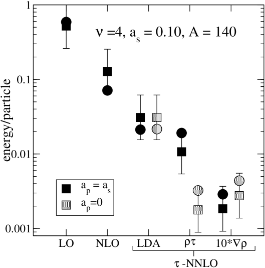
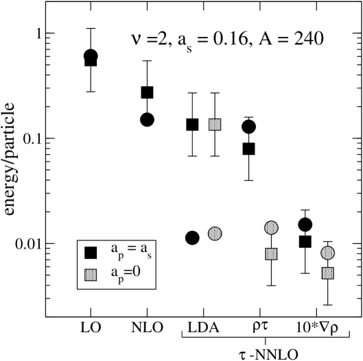
Figure 7: Energy estimates (squares and error bars) for $\nu=4$, $a_{s}=0.10$, $A=140$ particles compared with actual values (circles) for a hard-sphere gas (solid) and with the p-wave scattering length equal to zero (shaded).

Figure 8: Energy estimates (squares and error bars) for $\nu=2$, $a_{s}=0.16$, $A=240$ particles compared with actual values (circles) for a hard-sphere gas (solid) and with the p-wave scattering length equal to zero (shaded).

We see from Figs. 8 and 8 that the actual results for LO, NLO and NNLO agree well with NDA estimates, including the new gradient contributions, with one exception. The exception is the $\rho^{8/3}$ LDA estimate for the $\nu=2$ system, which greatly overestimates the actual contribution at that order due to an accidental cancellation when $\nu=2$ between the two terms in the $b_{4}$ coefficient in Eq. (47) PUG02 . In general, however, we can use these estimates to reliably predict the uncertainty in the energy per particle from higher orders.

While it’s clear that nuclei are not perturbative dilute Fermi systems with natural free-space scattering lengths, there is phenomenological evidence that power counting can apply to energy functionals that are fit to bulk nuclear properties. Phenomenologically successful functionals, both of the Skyrme type and covariant, have Hartree terms that are consistent with Georgi-Manohar NDA for a chiral low-energy theory Furnstahl:2001hs ; FURNSTAHL99b ; HACKWORTH . This involves power counting with two scales: the pion decay constant $f_{\pi}$ and an underlying scale for short-range physics $\Lambda$, which empirically (for these functionals) is around 600 MeV. (Equivalently, there is an additional large dimensionless coupling $g\sim\Lambda/f_{\pi}$ that enters in a well-prescribed manner). Thus the functionals do take the form of a density expansion (with parameter $\rho/f_{\pi}^{2}\Lambda$) as well as a gradient expansion, with the same hierarchy as illustrated here. A major goal of future investigations will be to elucidate the nature of the density expansion for finite nuclei and to connect it to the underlying chiral EFT.

IV Summary

In this paper, the EFT-based Kohn-Sham density functional for a confined, dilute Fermi gas was extended by incorporating the kinetic-energy-density $\tau({\bf\bf{x}})$ into the formalism. The generating functional is constructed by including, in addition to a source $J({\bf\bf{x}})$ coupled to the composite density operator $\psi^{\dagger}\psi$, another source $\eta({\bf\bf{x}})$ coupled to the (semi-local) kinetic energy density operator $\nabla\psi^{\dagger}\cdot\nabla\psi$. A functional Legendre transformation with respect to the sources yields an effective action of the kinetic energy density $\tau$ as well as the fermion density $\rho$. This construction also serves as a prototype for including additional densities currents (such as separate proton and neutron densities or a spin-orbit current).

This extension sets the stage for the construction of energy functionals and Kohn-Sham equations that go systematically beyond the local density approximation (LDA). As a first step, we included the exact Hartree-Fock (HF) contribution at NNLO for a natural dilute Fermi system but treated non-HF contributions in LDA. This exact HF contribution provides explicit dependence on $\tau$ and on the gradient of the density, unlike the LDA. The EFT expansion for a confined, finite system with natural effective range parameters is controlled by those parameters ($a_{s}$, $r_{s}$, $a_{p}$, …) times an average Fermi momentum and by the gradient of the density. Thus the expansion is perturbative in the sense of being a density expansion but is not perturbative in an underlying potential. (This is clear since our prototype system is hard spheres, which yields infinities even in first-order perturbation theory!) An error plot of contributions to the energy per particle versus the order of the calculation showed that we can reliably estimate the truncation error in a finite system, including the gradient terms.

The ground-state energy functional and Kohn-Sham single-particle equations constructed here take the same form as those in Skyrme Hartree-Fock calculations (not including the spin-orbit contribution, which can be added with a similar generalization). There is work supporting the Skyrme (and also covariant FURNSTAHL99b ) mean-field energy functionals as density expansions. Low-energy effective theories of QCD are expected to have a type of power counting. As shown in Ref. HACKWORTH , power counting in the energy functional based on chiral naive dimensional analysis is fully consistent with phenomenological parametrizations. The value of including the kinetic energy density as a functional variable is not conclusive in the present example, but it does lead to a single-particle spectrum closer to that of the exact Green’s function. In general, summing more nonlocalities without decreasing the numerical efficiency of the calculation is a plus.

Even in the simplest low-density expansion, there are contributions at all powers of the Fermi momentum, which means fractional powers of the density. In the Skyrme parametrization, there is only one such term. This is presumably a balance between phenomenological accuracy and a desire to maximize predictive power through limiting parameters. For reproducing bulk properties of stable nuclei, the Skyrme functional is only sensitive to a relatively small window in density, which allows significant freedom for a phenomenological parameterization. The future challenge will be to see if additional terms motivated by power counting, which may become important for extrapolating far from stability, can be determined.

The immediate next steps are to develop a derivative expansion to evaluate diagrams such as the NLO “beachball” diagram beyond LDA and to test it for convergence, and to generalize the DFT formalism to include pairing. Work is in progress on these extensions, which will be directly relevant for nuclear applications FURNSTAHL04 . In addition, in order to adapt the density functional procedure to chiral effective field theories with explicit pions, we will need to extend the discussion to include long-range forces. Kaiser, Weise, and collaborators have already generated functionals of the Skyrme type using free-space chiral perturbation theory together with the density matrix expansion of Negele et al. Kaiser:2002jz . It is not clear that the power counting is consistent in those calculations, but future development along these lines is certainly warranted. Finally, a systematic solution to the large scattering length problem for trapped atoms also remains a challenge.