Evolution of Hot, Dissipative Quark Matter in Relativistic Nuclear Collisions

Abstract

Non-ideal fluid dynamics with cylindrical symmetry in transverse direction and longitudinal scaling flow is employed to simulate the space-time evolution of the quark-gluon plasma produced in heavy-ion collisions at RHIC energies. The dynamical expansion is studied as a function of initial energy density and initial time. A causal theory of dissipative fluid dynamics is used instead of the standard theories which are acausal. We compute the parton momentum spectra and HBT radii from two-particle correlation functions. We find that, in non-ideal fluid dynamics, the reduction of the longitudinal pressure due to viscous effects leads to an increase of transverse flow and a decrease of the ratio $R_{out}/R_{side}$ as compared to the ideal fluid approximation.

1 Introduction

High-energy heavy-ion collisions offer the opportunity to study hot and dense nuclear matter [1]. Lattice QCD calculations [2] of thermodynamical functions indicate that, at zero net baryon number density, strongly interacting matter undergoes a rapid transition from (a chirally broken, confined) hadronic phase to a (chirally symmetric, deconfined) quark-gluon plasma (QGP). The transition temperature is found to be around $T_{c}\sim 160$ MeV. One of the primary goals of relativistic heavy-ion physics is the creation and observation of the predicted QGP.

Fluid dynamics is the only dynamical model which provides a direct link between collective observables and the equation of state. Besides, it can also be linked to microscopic models via the energy-momentum tensor or via the transport coefficients.

The applicability of ideal fluid dynamics rests on the assumption of local thermodynamic equilibrium. That is, in the local rest frame of the fluid the single-particle phase space distribution function is assumed to be isotropic in momentum space. However, for the early stage of a collision this may not be a very accurate approximation because the initial particle momenta are predominantly oriented in the longitudinal (beam) direction. Then it is necessary to account for the anisotropy of the phase space distribution in order to carry out a detailed analysis of the dynamics of the matter. Because of the anisotropy, shear viscous stresses arise. In the case of strongly interacting mixtures, in addition to shear and bulk viscous pressure, also diffusion has to be included in the analysis [3, 4].

While for ideal fluid dynamics we only consider the conservation equations, in non-ideal fluid dynamics we need to include a second set of transport equations. The standard theories of irreversible processes due to Eckart [5] or Landau [6] exhibit undesirable effects (i.e., they predict an infinite speed of propagation for thermal and viscous signals and unstable equilibrium states [7]). It is then necessary to resort to another non-ideal fluid-dynamical theory that does not have this anomalous behavior. Causal theories for non-ideal fluids were formulated by Müller [8] based on Grad’s 14-moment method [9] and written in relativistically covariant form by Israel and Stewart [10]. These are based upon extended irreversible thermodynamics, where the entropy current vector of standard thermodynamics is extended by including terms that are quadratic in the dissipative quantities. Causal fluid dynamics seems to be a good candidate to replace the standard Eckart or Landau theory. It has already been applied previously in Ref. [11] to one-dimensional Bjorken scaling flow [12].

In the present work we extend the investigation of Ref. [11] to more realistic, three-dimensional geometries. We consider a system consisting of quarks and gluons with an equation of state of an ultrarelativistic ideal gas. This implies that the bulk viscosity vanishes [13]. We also assume the system to be net baryon free. Consequently the heat flow is small and will be neglected. The dominant dissipative corrections are then due to shear viscosity. The evolution of the system is studied assuming transverse cylindrical symmetry and Bjorken scaling flow in the longitudinal direction. To explore observable consequences of non-ideal fluid behaviour, we calculate the transverse momentum distribution of the produced partons and the two-particle correlation functions in side-, out- and long-direction, giving rise to the so-called HBT radii $R_{side}$, $R_{out}$, and $R_{long}$. At this point, we do not consider the hadronization of partons since the transport coefficients in the mixed phase are unknown. Nevertheless, the present work is the first to solve the second order (and thus causal) equations of relativistic dissipative fluid dynamics for a realistic three-dimensional geometry. Previous attempts use the first order equations which are acausal as a matter of principle.

The remainder of the paper is organized as follows. In section 2 we briefly review the equations of causal non-ideal fluid dynamics in a general frame. In section 3 we present the relaxational transport equations necessary to solve non-ideal fluid dynamics (also in a general frame). In section 4 we explicitly present the equations for the Bjorken cylinder-type expansion. In section 5 we outline the initial conditions, equations of state and transport coefficients used in the calculations. In section 6 we discuss the freeze-out prescription for particle spectra and HBT radii. We also discuss the dissipative corrections to the distribution function. In section 7 we present our results for the spectra and HBT radii. In section 8 we summarize our work. Mathematical details are deferred to the Appendix.

Our units are $\hbar=c=k_{\rm B}=1$. The metric tensor is $g^{\mu\nu}=\mbox{diag}(+,-,-,-)$. The scalar product of two 4-vectors $a^{\mu},\,\,b^{\mu}$ is denoted by $a^{\mu}\,g_{\mu\nu}\,b^{\nu}\equiv a^{\mu}\,b_{\mu}$, and the scalar product of two 3-vectors ${a}$ and ${b}$ by $\mbox{\boldmath${a}$}\cdot\mbox{\boldmath${b}$}$. The notations $A^{(\alpha\beta)}\equiv(A^{\alpha\beta}+A^{\beta\alpha})/2$ and $A^{[\alpha\beta]}\equiv(A^{\alpha\beta}-A^{\beta\alpha})/2$ denote symmetrization and antisymmetrization, respectively. The 4-derivative is denoted by ${\partial}_{\alpha}\equiv{\partial}/{\partial}x^{\alpha}$. An overdot denotes $\dot{A}=u^{\lambda}{\partial}_{\lambda}A$.

2 Basics of non-ideal fluid dynamics

In this section we present the equations of causal non-ideal fluid dynamics. We consider a fluid that consists of a single conserved charge. For a mixture of several conserved charges see Ref. [4]. The variables of concern are the (net) charge current $N^{\mu}$, the energy-momentum tensor $T^{\mu\nu}$ and the entropy flux $S^{\mu}$. The divergence of the energy-momentum tensor and the charge current vanish, i.e., energy-momentum and charge are conserved. However, in general the divergence of the entropy current does not vanish. The second law of thermodynamics requires that it be a positive and nondecreasing function of time. In equilibrium the entropy is maximum and the divergence of the entropy current vanishes. Thus,

$${\partial}_{\mu}N^{\mu} = 0\enspace,$$ (1)

$${\partial}_{\nu}T^{\mu\nu} = 0\enspace,$$ (2)

$${\partial}_{\mu}S^{\mu} \geq 0\enspace,$$ (3)

where

$$N^{\mu} = nu^{\mu}+V^{\mu}\enspace,$$ (4)

$$T^{\mu\nu} = (\varepsilon+p+\Pi)u^{\mu}u^{\nu}-(p+\Pi)g^{\mu\nu}+2W^{(\mu}u^{\nu)}+\pi^{\mu\nu}\enspace,$$ (5)

$$S^{\mu} = su^{\mu}+\beta W^{\mu}-\alpha V^{\mu}-{1\over 2}\beta u^{\mu}\biggl{(}\beta_{0}\Pi^{2}-\bigl{[}\beta_{1}q^{\nu}q_{\nu}+{W^{\nu}W_{\nu}\over w}\bigr{]}+\beta_{2}\pi^{\lambda\nu}\pi_{\lambda\nu}\biggr{)}$$ (6)

$$~{}~{}~{}~{}~{}~{}~{}~{}~{}~{}~{}~{}~{}~{}~{}~{}~{}~{}~{}~{}~{}~{}~{}~{}~{}-\beta\biggl{(}\bigl{[}\alpha_{0}q^{\mu}+{W^{\mu}\over w}\bigr{]}\Pi-\bigl{[}\alpha_{1}q_{\nu}+{W_{\nu}\over w}\bigr{]}\pi^{\mu\nu}\biggr{)}\enspace.$$

In the local rest frame defined by $u^{\mu}=(1,\bf{0})$ the quantities appearing in the above tensors have the following meaning. Defining the projection operator $\bigtriangleup^{\mu\nu}\equiv g^{\mu\nu}-u^{\mu}u^{\nu}\equiv\bigtriangleup^{\nu\mu}$ onto the 3-space orthogonal to $u^{\mu}$, i.e., $\bigtriangleup^{\mu\nu}u_{\nu}=0$, $n\equiv u_{\mu}N^{\mu}$ is the net baryon number density, $V^{\mu}\equiv\bigtriangleup^{\mu}_{\nu}N^{\nu}$ is the net flow of charge, $\varepsilon\equiv u_{\mu}T^{\mu\nu}u_{\nu}$ is the energy density, $p+\Pi\equiv-\frac{1}{3}\bigtriangleup_{\mu\nu}T^{\mu\nu}$ is the local isotropic pressure plus bulk pressure, $W^{\mu}\equiv u_{\nu}T^{\nu\lambda}\bigtriangleup^{\mu}_{\lambda}$ is the energy flow, $q^{\mu}\equiv W^{\mu}-(w/n)V^{\mu}$ is the heat flow, $\pi^{\mu\nu}\equiv T^{\langle\mu\nu\rangle}$ is the stress tensor, and $s\equiv u_{\mu}\,S^{\mu}$ is the entropy density. The angular bracket notation, representing the symmetrized spatial and traceless part of the tensor, is defined by $A^{\langle\mu\nu\rangle}\equiv\left[\frac{1}{2}\left(\bigtriangleup^{\mu}_{\sigma}\bigtriangleup^{\nu}_{\tau}+\bigtriangleup^{\mu}_{\tau}\bigtriangleup^{\nu}_{\sigma}\right)-\frac{1}{3}\bigtriangleup^{\mu\nu}\bigtriangleup_{\sigma\tau}\right]A^{\sigma\tau}$. The space-time derivative decomposes into $\partial^{\mu}=u^{\mu}D+\bigtriangledown^{\mu}$, where $D\equiv u^{\mu}\partial_{\mu}$ is the comoving time derivative and $\bigtriangledown^{\mu}\equiv\bigtriangleup^{\mu\nu}\partial_{\nu}$ is the gradient operator. The quantity $\beta\equiv 1/T$ is the inverse temperature and $\alpha=\mu/T$ is the chemical potential times the inverse temperature. $w\equiv\varepsilon+p$ is the enthalpy density. The coefficients $\alpha_{i}(\varepsilon,n)$ and $\beta_{i}(\varepsilon,n)$ in Eq. (6) are thermodynamic integrals and given by the equation of state.

So far $u^{\mu}$ is an arbitrary 4-vector and is normalized such that $u^{\mu}u_{\mu}=1$ and therefore $u^{\mu}{\partial}_{\nu}u_{\mu}=0$. It can be taken to be the particle flow velocity. This is the Eckart frame. In this frame $V^{\mu}\equiv 0$. Alternatively, it can be taken to be the energy flow velocity. This is known as the Landau frame. In this frame $W^{\mu}\equiv 0$. The Landau or energy frame variables $\alpha_{i}$ and $\beta_{i}$ are related to the Eckart or particle frame variables $\bar{\alpha_{i}}$ and $\bar{\beta_{i}}$, respectively, by

$$\bar{\alpha_{i}}-\alpha_{i}=\bar{\beta_{1}}-\beta_{1}=w^{-1}\enspace,~{}~{}~{}~{}~{}\mbox{and}~{}~{}~{}~{}~{}\bar{\beta_{0}}=\beta_{0}~{}~{},~{}~{}~{}~{}~{}\bar{\beta_{2}}=\beta_{2}\enspace.$$ (7)

3 Transport Equations

In this section we present the transport equations for the independent dissipative fluxes $\Pi,q^{\mu},\pi^{\mu\nu}$. We shall consider the Landau frame where $W^{\mu}=0$ and thus $q^{\mu}=-(w/n)V^{\mu}$. We shall use the Müller-Israel-Stewart second-order theory for non-ideal fluids [8, 10], which is based on extended irreversible thermodynamics. Causal non-ideal fluid dynamics rests on two assumptions: (1) The dissipative flows (heat flow and viscous pressures) are considered as independent variables, hence, the entropy function depends not only on the standard variables, charge density and energy density, but also on these dissipative flows. (2) In equilibrium, the entropy function assumes a maximum. Moreover, its flow depends on all dissipative flows and its production rate is positive semi-definite. As a consequence the heat flow $q^{\mu}$, the bulk pressure $\Pi$ and the traceless shear viscous tensor $\pi^{\mu\nu}$ obey the evolution equations [10]

$$\tau_{\Pi}\dot{\Pi}+\Pi = -\zeta\bigtriangledown_{\mu}u^{\mu}-\frac{1}{2}\zeta T\Pi{\partial}_{\mu}\left(\frac{\tau_{\Pi}u^{\mu}}{\zeta T}\right)$$ (8)

$$+l_{\Pi q}\bigtriangledown_{\mu}q^{\mu}\enspace,$$

$$\tau_{q}\bigtriangleup_{\nu}^{\mu}\dot{q}^{\nu}+q^{\mu} = \kappa T\left(\frac{\bigtriangledown^{\mu}T}{T}-a^{\mu}\right)+\frac{1}{2}\kappa T^{2}q^{\mu}{\partial}_{\nu}\left(\frac{\tau_{q}u^{\nu}}{\kappa T^{2}}\right)$$ (9)

$$-l_{q\pi}\bigtriangledown_{\nu}\pi^{\mu\nu}-l_{q\Pi}\bigtriangledown^{\mu}\Pi+\tau_{q}\omega^{\mu\nu}q_{\nu}\enspace,$$

$$\tau_{\pi}\bigtriangleup^{\mu\alpha}\bigtriangleup^{\nu\beta}\dot{\pi}_{\alpha\beta}+\pi^{\mu\nu} = 2\eta\bigtriangledown^{\langle\mu}u^{\nu\rangle}-\frac{1}{2}\eta T\pi^{\mu\nu}{\partial}_{\lambda}\left(\frac{\tau_{\pi}u^{\lambda}}{\eta T}\right)$$ (10)

$$+l_{\pi q}\bigtriangledown^{\langle\mu}q^{\nu\rangle}+2\tau_{\pi}\pi^{\alpha(\mu}\omega^{\nu)}_{\alpha}\enspace,$$

where $\kappa$, $\zeta$, and $\eta$ denote the thermal conductivity, and the bulk and shear viscous coefficients, respectively. Also

$$\tau_{\Pi} = \zeta\beta_{0}\;\;,\;\;\tau_{q}=\kappa T\beta_{1}\;\;,\;\;\tau_{\pi}=2\eta\beta_{2}\enspace,$$ (11)

$$l_{\Pi q} = \zeta\alpha_{0}\;\;,\;\;l_{q\Pi}=\kappa T\alpha_{0}\;\;,\;\;l_{q\pi}=\kappa T\alpha_{1}\;\;,\;\;l_{\pi q}=2\eta\alpha_{1}\enspace,$$ (12)

are the relaxation times for the bulk pressure ($\tau_{\Pi}$), the heat flux ($\tau_{q}$), and the shear tensor ($\tau_{\pi}$) ; and the relaxation lengths for the coupling between heat flux and bulk pressure ($l_{\Pi q}$, $l_{q\Pi}$) and between heat flux and shear tensor ($l_{q\pi}$, $l_{\pi q}$). Since the bulk viscosity vanishes for an ultrarelativistic ideal gas [13] and since the heat flux will turn out to be negligible small, we shall only need the expression for $\beta_{2}$. $a^{\mu}\equiv\dot{u}^{\mu}$ is the 4- acceleration, and $\omega^{\mu\nu}\equiv\bigtriangleup^{\mu\alpha}\bigtriangleup^{\nu\beta}{\partial}_{[\beta}u_{\alpha]}$ is the vorticity tensor.

The standard theory of Landau is contained in these causal transport equations. To see this, set all relaxation time and length scales in Eqs. (8-10) to zero:

$$\Pi \equiv -\zeta\Theta\enspace,$$ (13)

$$q^{\mu} \equiv \kappa T\left(\frac{\bigtriangledown^{\mu}T}{T}-a^{\mu}\right)=-{\lambda\,n\,T^{2}\over w}\bigtriangledown^{\mu}\left(\frac{\mu}{T}\right)\enspace,$$ (14)

$$\pi^{\mu\nu} \equiv 2\eta\sigma^{\mu\nu}\enspace,$$ (15)

where $\Theta\equiv\bigtriangledown_{\mu}u^{\mu}$ is the expansion scalar, and $\sigma^{\mu\nu}\equiv\bigtriangledown^{\langle\mu}u^{\nu\rangle}=\bigtriangledown^{(\mu}u^{\nu)}-\frac{1}{3}\bigtriangleup^{\mu\nu}\bigtriangledown_{\lambda}u^{\lambda}$ is the shear tensor.

4 Longitudinal boost invariance with transverse expansion

We now consider the three-dimensional expansion with longitudinal boost invariance and cylindrical symmetry in transverse direction. We take the $z$-axis to be the beam direction and use cylindrical coordinates.

We are interested in the transverse motion. We will take advantage of the one-dimensional scaling solution which, under boosts along the longitudinal direction, is invariant. Thus we can go to a point (along the $z$-axis) where the equations are simple, for instance $z=0$, and derive the radial solution. Afterwards, one can boost this solution along the longitudinal direction. We use the coordinate transformations,

$$t=\tau\cosh\eta\;\;,\;\;z=\tau\sinh\eta\enspace,$$ (16)

where

$$\tau=\sqrt{t^{2}-z^{2}}\enspace,~{}~{}~{}~{}~{}~{}~{}~{}~{}~{}\eta=\frac{1}{2}\ln\frac{t+z}{t-z}\enspace.$$ (17)

We take matter to be net baryon free, and thus $N^{\mu}\equiv 0$. Therefore we do not need to consider Eq. (1). The energy-momentum tensor in the local rest frame is

$$\hat{T}^{\mu\nu} = \left(\varepsilon+{\cal P}_{\perp}\right)\hat{u}^{\mu}\hat{u}^{\nu}-{\cal P}_{\perp}g^{\mu\nu}+\left({\cal P}_{z}-{\cal P}_{\perp}\right)\hat{l}^{\mu}\hat{l}^{\nu}+\left({\cal P}_{r}-{\cal P}_{\perp}\right)\hat{m}^{\mu}\hat{m}^{\nu}$$ (18)

$$+2\tau^{rz}\hat{l}^{(\mu}\hat{m}^{\mu)}+2W^{r}\hat{u}^{(\mu}\hat{m}^{\nu)}+2W^{z}\hat{u}^{(\mu}\hat{l}^{\nu)}\enspace,$$

where ${\cal P}_{r}\equiv p+\tau^{rr}+\Pi$, ${\cal P}_{z}\equiv p+\tau^{zz}+\Pi$, ${\cal P}_{\perp}={\cal P}_{\phi}\equiv p+\tau^{\phi\phi}+\Pi$ and

$$\hat{u}^{\mu}(r,\eta,\tau) = (1,0,0,0)\enspace,$$ (19)

$$\hat{l}^{\mu}(r,\eta,\tau) = (0,0,0,1)\enspace,$$ (20)

$$\hat{m}^{\mu}(r,\eta,\tau) = (0,\mbox{\boldmath${e}$}_{r},0)\enspace,$$ (21)

with

$$\mbox{\boldmath${e}$}_{r}=(\cos\phi,\sin\phi)\enspace.$$ (22)

The $\tau^{ij}$ and $W^{i}$ are the components of $\pi^{\mu\nu}$ and the $W^{\mu}$ in the local rest frame. Due to scaling assumption the component $\tau^{rz}$ will not contribute at $z=0$ or $\eta=0$. For the same reason $W^{z}$ will not contribute.

Successive boosts with radial fluid flow velocity $v_{r}=v_{r}(r,\tau)$ in the transverse direction and with Bjorken fluid flow velocity $v_{z}=\tanh\eta$ in the longitudinal ($z$-axis) direction give

$$T^{\mu\nu} = \left(\varepsilon+{\cal P}_{\perp}\right)u^{\mu}u^{\nu}-{\cal P}_{\perp}g^{\mu\nu}+\left({\cal P}_{z}-{\cal P}_{\perp}\right)l^{\mu}l^{\nu}+\left({\cal P}_{r}-{\cal P}_{\perp}\right)m^{\mu}m^{\nu}$$ (23)

$$+2\tau^{rz}l^{(\mu}m^{\mu)}+2W^{r}u^{(\mu}m^{\nu)}+2W^{z}u^{(\nu}l^{\nu)}\enspace,$$

with

$$u^{\mu}(r,\eta,\tau) = \gamma(\cosh\eta,v_{r}\mbox{\boldmath${e}$}_{r},\sinh\eta)\enspace,$$ (24)

$$l^{\mu}(r,\eta,\tau) = (\sinh\eta,0,0,\cosh\eta)\enspace,$$ (25)

$$m^{\mu}(r,\eta,\tau) = \gamma(v_{r}\cosh\eta,\mbox{\boldmath${e}$}_{r},v_{r}\sinh\eta)\enspace,$$ (26)

where $\gamma\equiv 1/\sqrt{1-v_{r}^{2}}$. The set of three 4-vectors has the following properties: $u^{\mu}$ is timelike, $u^{\mu}u_{\mu}=1$, and the other two, $l^{\mu}$ and $m^{\mu}$, are spacelike $l^{\mu}l_{\mu}=m^{\mu}m_{\mu}=-1$. The three are orthogonal $u^{\mu}l_{\mu}=u^{\mu}m_{\mu}=l^{\mu}m_{\mu}=0$. The energy flux is given by

$$W^{\mu}=W^{r}u^{(\mu}m^{\nu)}+W^{z}u^{(\mu}l^{\nu)}\enspace.$$ (27)

and due to the symmetry of the problem (no energy flow in the $z$-direction at $z=0$) only the radial part remains and we will simply denote it by $W$, i.e. $W\equiv W^{r}$. The shear stress tensor takes the form

$$\pi^{\mu\nu}=\left(\begin{matrix}\Pi^{rz}\cosh^{2}\eta-\tau^{zz}&\tau^{rr}\gamma^{2}v_{r}\cos\phi\cosh\eta&\tau^{rr}\gamma^{2}v_{r}\sin\phi\cosh\eta&\Pi^{rz}\cosh\eta\sinh\eta\\ \tau^{rr}\gamma^{2}v_{r}\cos\phi\cosh\eta&\Pi^{r\phi}\cos^{2}\phi+\tau^{\phi\phi}&\Pi^{r\phi}\cos\phi\sin\phi&\tau^{rr}\gamma^{2}v_{r}\cos\phi\sinh\eta\\ \tau^{rr}\gamma^{2}v_{r}\sin\phi\cosh\eta&\Pi^{r\phi}\cos\phi\sin\phi&\Pi^{r\phi}\sin^{2}\phi+\tau^{\phi\phi}&\tau^{rr}\gamma^{2}v_{r}\sin\phi\sinh\eta\\ \Pi^{zr}\cosh\eta\sinh\eta&\tau^{rr}\gamma^{2}v_{r}\cos\phi\sinh\eta&\tau^{rr}\gamma^{2}v_{r}\sin\phi\sinh\eta&\Pi^{zr}\cosh^{2}\eta-\tau^{rr}\gamma^{2}v_{r}^{2}\end{matrix}\right)\enspace,$$ (28)

where $\Pi^{rz}=\Pi^{zr}=\tau^{rr}\gamma^{2}v_{r}^{2}+\tau^{zz}$ and $\Pi^{r\phi}=\Pi^{\phi r}=\tau^{rr}\gamma^{2}-\tau^{\phi\phi}$.

Note that in writing Eq. (28) we have omitted the $\tau^{rz}$ terms, since they will not contribute due to scaling at $z=0$ or at $\eta=0$. For the same reason the component $\pi^{rz}$ will not contribute.

The components of $T^{\mu\nu}$ which will be used in the following are $T^{00}$ and $T^{0r}$. At $\eta=z=0$ they take the form:

$$T^{00} = {\cal W}\gamma^{2}-{\cal P}_{r}+2W\gamma^{2}v_{r}\enspace,$$ (29)

$$T^{0r} = {\cal W}\gamma^{2}v_{r}+W\gamma^{2}(v_{r}^{2}+1)\enspace,$$ (30)

with ${\cal W}\equiv\varepsilon+{\cal P}_{r}$.

The equations of motion at $z=\eta=0$ reduce to

$${{\partial}\over{\partial}\tau}T^{00} = -{{\partial}\over{\partial}r}\left\{(T^{00}+{\cal P}_{r})v_{r}+W\right\}$$ (31)

$$~{}~{}~{}~{}~{}~{}~{}~{}~{}~{}~{}~{}~{}~{}~{}-\;(T^{00}+{\cal P}_{r}){\cal S}+({\cal P}_{r}-{\cal P}_{z}){1\over\tau}-W{1\over r}\enspace,$$

$${{\partial}\over{\partial}\tau}T^{0r} = -{{\partial}\over{\partial}r}\left\{(T^{0r}+W)v_{r}+{\cal P}_{r}\right\}$$ (32)

$$~{}~{}~{}~{}~{}~{}~{}~{}~{}~{}~{}~{}~{}~{}~{}-T^{0r}{\cal S}-({\cal P}_{r}-{\cal P}_{\phi}){1\over r}-W{v_{r}\over r}\enspace,$$

where

$${\cal S}\equiv\frac{v_{r}}{r}+\frac{1}{\tau}\enspace.$$ (33)

The velocity and local energy density are given by

$$v_{r} = {T^{0r}-W\over T^{00}+{\cal P}_{r}}\enspace,$$ (34)

$$\varepsilon = T^{00}-{\left(T^{0r}\right)^{2}-\left(W\right)^{2}\over T^{00}+{\cal P}_{r}}\enspace.$$ (35)

For an equation of state of the form $p=\varepsilon/3$ the energy density is determined from

$$\varepsilon=-\biggl{(}T^{00}+\frac{3}{2}\tau^{rr}\biggr{)}+\sqrt{4{T^{00}}^{2}-3\biggl{[}\left(T^{0r}\right)^{2}-\left(W\right)^{2}\biggr{]}+6T^{00}\tau^{rr}+\frac{9}{4}\left(\tau^{rr}\right)^{2}}\enspace.$$ (36)

Note that in the Landau frame $W=0$, and in the Eckart frame $W=q$.

We now consider the transport equations for the dissipative fluxes. These arise from the second law of thermodynamics, Eq. (3) [8, 10]. Note that, due to the symmetry of the problem, Eq. (9) has one independent component and Eq. (10) has two independent components. We shall take as equation of state $p=\varepsilon/3$, cf. section 5, and this implies that we do not need to consider the equation for the bulk pressure, since the bulk viscosity coefficient vanishes for this equation of state [13]. Consequently, $\Pi=0$, cf. Eq. (8). We also take the net charge to be zero, $n=0$. It is then convenient to work in the Landau frame. Since $n=0$, the driving force term in the heat flux equation (the first term on the right-hand side) vanishes, cf. Eq. (14). Although the remaining terms need not vanish, we checked that they are numerically small and thus we shall not consider the heat flux equation (9). Thus we are only left with the equation for the shear stress tensor, $\pi^{\mu\nu}$. After using the cylindrical symmetry the various components of Eq. (10) decouple and reduce to:

$${{\partial\over\partial\tau}}\tau^{rr} = -v_{r}{\partial\over\partial r}\tau^{rr}-\pi^{rr}{1\over\gamma\tau_{\pi}}+{2\eta\over\gamma\tau_{\pi}}\sigma^{rr}-{1\over 2\gamma}\tau^{rr}\biggl{[}\Theta-{5\over 4}{\dot{\varepsilon}\over\varepsilon}\biggr{]}\enspace,$$ (37)

$${{\partial\over\partial\tau}}\tau^{\phi\phi} = -v_{r}{\partial\over\partial r}\tau^{\phi\phi}-\tau^{\phi\phi}{1\over\gamma\tau_{\pi}}+{2\eta\over\gamma\tau_{\pi}}\sigma^{\phi\phi}-{1\over 2\gamma}\tau^{\phi\phi}\biggl{[}\Theta-{5\over 4}{\dot{\varepsilon}\over\varepsilon}\biggr{]}\enspace,$$ (38)

$${{\partial\over\partial\tau}}\tau^{zz} = -v_{r}{\partial\over\partial r}\tau^{zz}-\tau^{zz}{1\over\gamma\tau_{\pi}}+{2\eta\over\gamma\tau_{\pi}}\sigma^{zz}-{1\over 2\gamma}\tau^{zz}\biggl{[}\Theta-{5\over 4}{\dot{\varepsilon}\over\varepsilon}\biggr{]}\enspace.$$ (39)

Here

$$\Theta \equiv \theta+\gamma\left[\frac{1}{\tau}+\frac{v_{r}}{r}\right]\enspace,$$ (40)

$$\theta \equiv {{\partial\over\partial\tau}}\gamma+{{\partial\over\partial r}}\gamma v_{r}$$ (41)

$$\dot{f} \equiv \left[\gamma{{\partial\over\partial\tau}}+\gamma v_{r}{{\partial\over\partial r}}\right]f\enspace,$$ (42)

$$\sigma^{rr} \equiv -\theta+\frac{1}{3}\Theta\enspace,$$ (43)

$$\sigma^{\phi\phi} \equiv -\gamma{v_{r}\over r}+{1\over 3}\Theta\enspace,$$ (44)

$$\sigma^{zz} \equiv -\gamma{1\over\tau}+\frac{1}{3}\Theta\enspace.$$ (45)

The coupled system of conservation equations and transport equations is solved numerically using the code called LCPFCT [14]. It solves generalized continuity equations of the form

$${\partial\over\partial t}U=-{1\over r^{\alpha-1}}{\partial\over\partial r}\left\{r^{\alpha-1}Uv\right\}-{1\over r^{\alpha-1}}{\partial\over\partial r}\left\{r^{\alpha-1}D_{1}\right\}+C_{2}{\partial\over\partial r}D_{2}+D_{3}\enspace,$$ (46)

with $\alpha=1,2,3$ for Cartesian, cylindrical or spherical coordinates, respectively. The advantage of LCPFCT in the present application is that the additional source terms are included by means of the terms $D_{1}$, $D_{2}$ and $D_{3}$. The same set of coupled equations can be solved numerically using the RHLLE [15] or SHASTA [16] algorithms.

5 Initial Conditions, Equation of state and transport coefficients

For the initial energy density distribution in the transverse plane we use the Woods-Saxon parameterization

$$\varepsilon(r)=\varepsilon_{0}{1\over e^{(r-R_{0})/a}+1}\enspace,$$ (47)

with $R_{0}=1.14A^{1/3}$ fm and $a=0.54$ fm. Since we consider Au+Au collisions at RHIC, $A=197$. Here $\varepsilon_{0}$ is the maximum energy density for central collisions at an initial time $\tau_{0}$. The numerical value of $\varepsilon_{0}$ is determined from the equation of state $\varepsilon_{0}=3aT_{i}^{4}$, where $a$ is given in Eq. (48) and $T_{i}$ is the initial temperature. We will compare the ideal and non-ideal fluid dynamics results for similar initial conditions.

In non-ideal fluid dynamics we also need to specify, independently, the initial conditions for the dissipative fluxes. The independent components of the shear tensor are initialized to $\tau^{rr}=\tau^{\phi\phi}=\varepsilon(r)/18\,,\,\,\tau^{zz}=-\varepsilon(r)/9$, where $\varepsilon(r)$ is given in Eq. (47). These particular values can be motivated by a microscopic model study [17].

For this exploratory study a simple equation of state is used, namely that of an ultrarelativistic gas of massless $u\,,d\,,s\,$ quarks and gluons. Since the net charge is considered to be zero, the pressure is given by $p=aT^{4}$, and the entropy density by $s=4aT^{3}$, where

$$a=\left(16+\frac{21}{2}N_{f}\right)\frac{\pi^{2}}{90}\enspace,$$ (48)

is a constant determined by the number of quark colors and flavors and the number of gluon colors. Here $N_{f}$ is the number of quark flavors, taken to be $3$. The only relaxation coefficient we need is $\beta_{2}$ which, for massless particles, is given by [10]

$$\beta_{2}=\frac{3}{4p}\enspace.$$ (49)

The shear viscosity is given by [18, 19] $\eta=bT^{3}$ where

$$b=\left(1+1.70N_{f}\right)\frac{0.342}{(1+N_{f}/6)\,\alpha_{s}^{2}\ln(\alpha_{s}^{-1})}\enspace,$$ (50)

is a constant determined by the number of quark flavors and the number of gluon colors. The strong coupling constant, $\alpha_{s}$, is taken to be $0.5$.

In Fig. 1 we show the profiles for the components of the shear stress tensor as a function of the radial coordinates at different times.

Figure 1: The components of the shear stress tensor in units of $p_{0}=\varepsilon_{0}/3$ as a function of $r/R_{0}$, where $R_{0}$ is the initial radius of the system, at different times $t=\tau_{i}+n\Delta t$, $\Delta t=0.025$ fm/c.

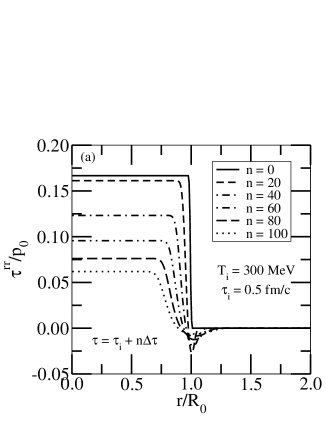
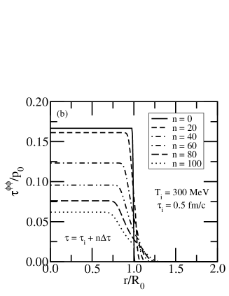
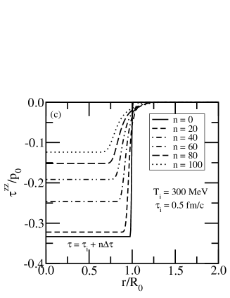
The effect of shear stress is to reduce the longitudinal pressure (hence $\tau^{zz}$ is negative) and to increase the transverse pressure (hence $\tau^{rr}$ and $\tau^{\phi\phi}$ are positive). Note that at any point in time the sum of the three components is zero. This reflects the tracelessness of the shear stress tensor.

6 Transverse spectra and HBT radii

To calculate single inclusive particle spectra or two-particle correlation functions in the fluid-dynamical framework, one assumes that a fluid element decouples from the fluid evolution, i.e., freezes out, as soon as the particle density drops below a certain critical value where the collision rate becomes too small to maintain local thermodynamic equilibrium. In our case, the particle density depends on the temperature only. Therefore, freeze-out happens across isotherms in the space-time diagram.

To calculate two-particle correlation functions we use the method developed by Pratt [20] and others, and applied to hydrodynamics in Ref. [21]. This method is a generalization of the Cooper-Frye formula [22] for single-inclusive particle spectra.

6.1 Freeze-out prescription

Just as in ideal hydrodynamics, our fluid-dynamical model describes the time evolution of macroscopic thermodynamic quantities which must be converted to particle spectra before one can compare with experimental data. To do so we use the well-known Cooper-Frye prescription [22] which gives the particle spectrum in terms of an integral over the phase-space distribution function along a so-called freeze-out hypersurface $\Sigma(x)$:

$$E\frac{\mbox{d}N}{\mbox{d}^{3}p}=\frac{\mbox{d}N}{\mbox{d}y\,\mbox{d}^{2}p_{\perp}}=\int_{\Sigma}\mbox{d}\Sigma_{\mu}(x)\,p^{\mu}\,f(x,p)\,,$$ (51)

$\mbox{d}\Sigma_{\mu}(x)$ is the 4-vector integral measure normal to the hypersurface and, in the case of ideal hydrodynamics, $f(x,p)$ is a local equilibrium distribution function of the form

$$f^{eq}(x,p)=A_{0}\left[\mbox{exp}(\beta u_{\mu}p^{\mu}-\alpha)-\epsilon\right]^{-1}\enspace,$$ (52)

where $A_{0}=g/(2\pi)^{3}$ and $\epsilon$ corresponds to the statistics of Boltzmann $(\epsilon=0)$, Bose $(\epsilon=+1)$, or Fermi $(\epsilon=-1)$. The degeneracy factor is $g=2J+1$, where $J$ is the spin of the particle. The flow velocity $u^{\mu}$ is evaluated along the freeze-out hypersurface $\Sigma$ and the temperature $T$ is calculated from the energy density on $\Sigma$. Longitudinal boost-invariance dictates freeze-out along a surface of fixed longitudinal proper time $\tau_{f}(r)$.

In general the freeze-out surface $\Sigma_{f}$ is a 3-dimensional hypersurface in space-time which can be parametrized by three orthogonal coordinates $\Sigma^{\mu}(u,w,v)$. The normal vector on the hypersurface is determined by

$$\mbox{d}\Sigma_{\mu}=-\epsilon_{\mu\nu\lambda\rho}{{\partial}\Sigma^{\nu}\over{\partial}u}{{\partial}\Sigma^{\lambda}\over{\partial}v}{{\partial}\Sigma^{\rho}\over{\partial}w}\enspace,$$ (53)

where $\epsilon^{\mu\nu\lambda\rho}=-\epsilon_{\mu\nu\lambda\rho}$ is totally antisymmetric, and $\epsilon^{\mu\nu\lambda\rho}=+1$ if $(\mu\nu\lambda\rho)$ is an even permutation of $(0,1,2,3)$.

6.2 Two Particle Correlations and HBT Radii

The two-particle correlation function for bosons can be written as [21]

$$C_{2}(p_{1},p_{2})=1+{\left|\int_{\Sigma}\mbox{d}\Sigma^{\mu}K_{\mu}\,\exp[iq_{\nu}\Sigma^{\nu}]\,f(x,p)\right|^{2}\over E_{1}\displaystyle{{\mbox{d}N\over\mbox{d}^{3}p_{1}}}E_{2}\displaystyle{{\mbox{d}N\over\mbox{d}^{3}p_{2}}}}\enspace,$$ (54)

where $K^{\mu}=(p_{1}^{\mu}+p_{2}^{\mu})/2$ is the average 4-momentum and $q^{\mu}=p_{1}^{\mu}-p_{2}^{\mu}$ is the relative 4-momentum. The symmetry of the problem reduces the number of independent variables on which $C_{2}$ depends. For particles emitted at midrapidity, $K^{z}=0$. Due to cylindrical symmetry around the $z$-axis we can choose the average transverse momentum as $K_{\perp}=(K,0,0)$ and the relative momenta as $q_{out}=(q_{out},0,0)$, $q_{side}=(0,q_{side},0)$ and $q_{long}=(0,0,q_{long})$.

For a fixed average transverse momentum $K$ we define side-, out-, and long-correlation functions as $C_{2,side}\equiv C_{2}(K,0,q_{side},0)$, $C_{2,out}\equiv C_{2}(K,q_{out},0,0)$, and $C_{2,long}\equiv C_{2}(K,0,0,q_{long})$, respectively. Then we define the corresponding inverse widths as $R_{side}\equiv\sqrt{\,\ln 2}/q_{side}^{*}$, $R_{out}\equiv\sqrt{\,\ln 2}/q_{out}^{*}$ and $R_{long}\equiv\sqrt{\,\ln 2}/q_{long}^{*}$, where $q_{side}^{*}$ is determined from $C_{2,side}(q_{side}^{*})=3/2$, and similarly for $q_{out}^{*}$ and $q_{long}^{*}$.

6.3 Dissipative corrections to the distribution function

For a gas that departs slightly from local thermal equilibrium, we may choose (independently at each point $x$) a local equilibrium distribution $f^{eq}(x,p)$ of the form (52), that is close to the actual distribution $f(x,p)$ and set

$$f(x,p)=f^{eq}(x,p)\left\{1+\Delta^{eq}\phi(x,p)\right\}\enspace,$$ (55)

where the Bose (Pauli) enhancement (blocking) factors are represented by

$$\Delta\equiv 1+\epsilon A_{0}^{-1}f\enspace,$$ (56)

where $A_{0}$ was defined below Eq. (52) and $\Delta^{eq}$ is given by replacing $f$ on the right hand side by $f^{eq}$. In the calculations of single particle spectra and two particle correlations we shall put $\Delta^{eq}=1$, ignoring the effects of Bose enhancement and Pauli blocking. This is justified because the dissipative corrections are small.

In macroscopic dynamics we seek a truncated hydrodynamical linearized description of small departures from equilibrium in which only the 14 variables $N^{\mu}$ and $T^{\mu\nu}$ appear. The microscopic counterpart of this is a truncated description in which the function

$$y(x,p)=\ln\left[A_{0}^{-1}f(x,p)/\Delta\right]\enspace,$$ (57)

differs from any nearby local equilibrium value

$$y_{eq}(x,p)=\alpha(x)-\beta(x)u_{\mu}(x)p^{\mu}\enspace,$$ (58)

by a function of momenta specifiable by 14 parameters.

The truncated description is derived via Grad’s relativistic 14-moment approximation [9, 10], or via a variational method [23], namely that $y-y_{eq}$ can be locally approximated by a quadratic function of 4-momentum,

$$\phi(x,p)\equiv y-y_{eq}\simeq\epsilon(x)-\epsilon_{\mu}(x)p^{\mu}+\epsilon_{\mu\nu}(x)p^{\mu}p^{\nu}\enspace,$$ (59)

where $\epsilon(x)$, $\epsilon_{\mu}(x)$, and $\epsilon_{\mu\nu}(x)$ are small. Without loss of generality $\epsilon_{\mu\nu}$ may be taken to be traceless, since its trace can be absorbed in a redefinition of $\epsilon$. The non-equilibrium distribution function (55) depends on the 14 variables $\alpha-\epsilon\,,\beta u_{\mu}+\epsilon_{\mu}\,,\epsilon_{\mu\nu}$. These parameters are related to the dissipative fluxes. For a system which only experiences shear stress we just need to know [10]

$$\epsilon_{\mu\nu}={\cal C}\pi_{\mu\nu}\enspace,$$ (60)

where the coefficient ${\cal C}$ is given by

$${\cal C}={\beta^{2}\over 2w}\enspace.$$ (61)

7 Non-ideal versus ideal fluid dynamics

Since we do not consider hadronization in our model studies we do not follow the dynamics beyond the hadronization point. We stop the dynamical evolution and calculate the spectra along a surface of constant energy density $\varepsilon_{f}$ or along given space-time isotherms. By truncating the dynamics before hadronization we cannot compare our results directly with experiment. Nevertheless, we can estimate the effects of entropy production in the non-ideal fluid-dynamical evolution by comparing the spectra with the ones obtained in ideal fluid dynamics. Let us note that an additional 7.5% [24] to 25% [25] increase in entropy is expected to arise in the hadronization transition, but this occurs in the non-ideal as well as in the ideal case. By neglecting the hadronization transition, we of course underestimate the total amount of produced entropy and, consequently, the final hadron multiplicity.

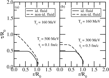
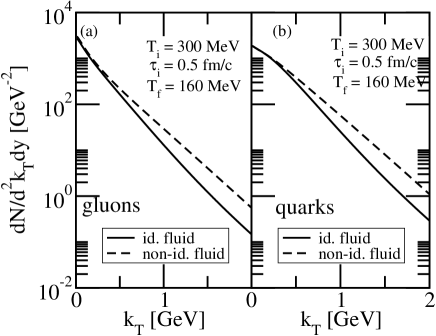
We present here the fluid-dynamical expansion solutions for a Bjorken cylinder geometry for different initial energy densities $\varepsilon_{0}$ and initial $\tau_{0}$. We study two scenarios. The first corresponds to a central Au+Au collision at RHIC, where the transverse radius of the hot zone is of order of 5 fm, while the time scale of local equilibration is roughly given by the energy loss of a parton interacting with matter, $\tau_{\mbox{d}E/\mbox{d}x}\approx 0.5$ fm [26]. Consequently, we choose $\tau_{0}=0.1R_{0}$ [21]. For the initial energy density we take an exemplary value of $\varepsilon_{0}=25$ GeV/fm^-3. For the second scenario we consider $\tau_{0}=1/3T_{0}$ which is motivated by an uncertainty principle argument [27]. In this case we take $\varepsilon_{0}=100$ GeV fm^-3, which corresponds to the maximum energy density reached in VNI(PCM) simulations [28]. We use the same initial conditions for the non-ideal and ideal fluid-dynamical calculations. In this way, the dissipative effects on the evolution can be observed most clearly. Since we do not consider hadronization we do not make an attempt to reproduce actual experimental data, which could require a readjustment of the initial conditions.

In Fig. 2 we show the freeze-out time $\tau_{f}(r)$, defined by $\varepsilon_{f}$ or, equivalently, by $T_{f}$, as a function of position in the transverse plane. Due to the strong initial longitudinal motion, the system cools rather quickly even before the transverse rarefaction waves reaches the center of the cylinder. The duration of the expansion is therefore solely determined by the longitudinal scaling expansion. This causes the horizontal parts of the isotherms. The effect of longitudinal cooling is reduced for larger values of $\tau_{0}$. One observes that for identical initial conditions ideal fluid dynamics leads to earlier freeze-out. The longer freeze-out times in non-ideal fluid dynamics originate from the fact that the longitudinal pressure is reduced due to viscosity effects, cf. Fig. 1.

Figure 2: The freeze-out time $\tau_{f}(r)$ as a function of transverse coordinate $r$. (a) VNI scenario, (b) RHIC scenario.

In Fig. 3 we show the parton transverse momentum spectra. Due to longer freeze-out times in non-ideal fluid dynamics, the corresponding spectrum is enhanced at high $p_{T}$. The reason is that non-ideal fluid dynamics creates stronger radial flow than ideal fluid dynamics due the increase of the transverse and the decrease of the longitudinal pressure, see Fig. 1. Similar results on the space-time isotherms and the transverse momentum spectra were found [29] by considering ideal hydrodynamics of a transversally thermalized system of gluons.

Figure 3: Parton $p_{\perp}$ distribution for the RHIC scenario.

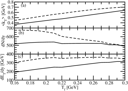
In Fig. 4 we show the parton mean transverse momentum, multiplicity and transverse energy as a function of freeze-out temperature for the RHIC scenario. Decreasing freeze-out temperature corresponds to increasing freeze-out time. For both the ideal and non-ideal evolution, the mean transverse momentum decreases with increasing freeze-out time. The reason is that, for massless particles, the decrease of the temperature has a stronger influence than the increase of the radial flow. One also observes that the stronger radial motion in the non-ideal case increases the mean transverse momentum as compared to the ideal case. Note that the initial value of the transverse momentum in the non-ideal case differs from that in the ideal case because of the dissipative corrections to the single particle distribution function.

In ideal fluid dynamics entropy is conserved, $\mbox{d}S/\mbox{d}y=constant$. For massless partons, the entropy density is proportional to the number density and thus $\mbox{d}N/\mbox{d}y\sim\mbox{d}S/\mbox{d}y$. Therefore, $\mbox{d}N/\mbox{d}y$ should be constant as a function of $T_{f}$. The 10% deviation from this relation observed in Fig. 4(b) for the ideal fluid case is caused partially by the numerical viscosity generated in the course of the evolution and partially by the numerical uncertainty introduced when integrating the single particle spectra over transverse momentum. In non-ideal fluid dynamics the entropy per unit rapidity $\mbox{d}S/\mbox{d}y$ increases with time (i.e., decreases with $T_{f}$) and so does $\mbox{d}N/\mbox{d}y$. Longitudinal boost invariance implies that the total transverse energy per unit rapidity, $\mbox{d}E_{\perp}/\mbox{d}y$, is independent of $y$. Due to the reduced longitudinal pressure in non-ideal hydrodynamics, the longitudinal work performed is also reduced and $\mbox{d}E_{\perp}/\mbox{d}y$ decreases more slowly with freeze-out time in comparison with ideal fluid dynamics.

Figure 4: The mean transverse momentum (a), multiplicity (b) and transverse energy (c). The solid curves are for the ideal fluid evolution and the dashed curves are for the non-ideal fluid evolution.

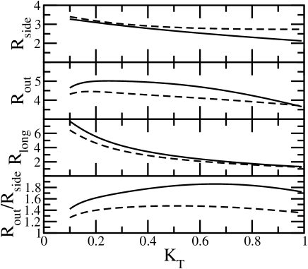
In Fig. 5 we show the $K_{\perp}$ dependence of HBT radii and the ratio $R_{out}/R_{side}$. The consequence of the longitudinal pressure reduction is to reduce the longitudinal radius $R_{long}$. The widths of the correlation functions correspond to the space-time structure of the corresponding isotherms. The effect of dissipation is to reduce $R_{out}$ while at the same time increasing $R_{side}$. This leads to the reduction of the ratio $R_{out}/R_{side}$ and this works in favor of reproducing experimental data which are overestimated by ideal fluid dynamics [30, 31, 32, 33]. For discussions on the effects of first order viscous corrections to ideal hydrodynamical description on spectra, elliptic flow and HBT radii see Ref. [33]. Fig.5 is obtained with the freeze-out temperature of 110 MeV for pions of mass 138 MeV.

Figure 5: HBT radii and the ratio $R_{out}/R_{side}$. The solid curves are for the ideal fluid and the dashed curves are for the non-ideal fluid.

8 Conclusions and Outlook

In this work we have compared the evolution of a non-ideal fluid of massless partons with that of an ideal fluid. We solved the fluid dynamical equations in a realistic 3+1 dimensional geometry appropriate for central Au+Au collisions at RHIC energies, i.e., assuming cylindrical symmetry in the transverse direction and boost invariance in the longitudinal direction. We have used similar initial conditions in the ideal and non-ideal case. Since our model only contains partons and lacks a description of hadronization, we truncated the evolution of the system just before the onset of hadronization, at a (fictitious) freeze-out temperature of $T_{f}\geq 160$ MeV.

We then investigated the influence of viscosity on the transverse momentum spectra, the parton multiplicity, the transverse energy, as well as the HBT radii. We found that the reduction of longitudinal pressure in the non-ideal case leads to an increase in radial flow. This has the consequence that, for comparable freeze-out temperatures, the mean transverse momentum is larger in the non-ideal case by $\sim 100$ MeV. Another consequence is that the longitudinal HBT radius $R_{long}$ is reduced. Simultaneously, $R_{side}$ increases while $R_{out}$ decreases. All this works in favour of reproducing experimental data, although we refrain from a detailed comparison to the latter due to the lack of hadronization in our model.

Finally, dissipation produces entropy and consequently the final parton multiplicity increases in the non-ideal case as compared to the ideal case where it should stay constant on account of entropy conservation. In the ideal case longitudinal work decreases the transverse energy $\mbox{d}E_{T}/\mbox{d}y$ with increasing freeze-out time. This decrease is considerably smaller in the non-ideal case due to the reduction of the longitudinal pressure.

For the future, it is important to extend our considerations to finite baryon densities, and to include the hadronization of partons. In order to model hadronization in fluid dynamics one has to consider an equation of state with a phase transition from hadronic matter to quark-gluon plasma. In the mixed phase the bulk viscosity coefficients can be large and comparable to the shear viscosity coefficient. This in turn will have a significant effect on the life time of the system, thereby affecting observables such as the HBT radii. The final hadron spectra have to be computed along a freeze-out surface in the hadronic phase. Only then a realistic comparison of the model results to experimental data is possible.

In order to reproduce the experimental data one will be forced to adjust the initial conditions. We expect that the latter will be very different in the non-ideal as compared to the ideal case. Our results for the evolution of a purely partonic phase indicate that a better simultaneous description of particle spectra and HBT radii is possible. Another important observable which should be reproduced within the fluid dynamical framework is the elliptic flow. This cannot be studied in the present cylindrically symmetric scenario; we have to generalize our study to allow for non-symmetric configurations in the transverse plane.

Appendix A Particle spectra and HBT radii from a cylindrically symmetric freeze-out surface

In this Appendix we calculate the particle spectrum, and the out-, side-, and long-correlations in the Bjorken cylinder geometry. This is a generalization of Appendix B of Ref. [21] to include dissipation in particle spectra and two- particle correlation functions. Due to boost invariance, the surface is simply the space-time hyperbola of constant $\tau_{f}=\sqrt{\tau_{f}^{2}-z_{f}^{2}}$. Note that at $z=0$, $\tau_{f}$ depends only on $r_{f}$, $\tau_{f}=\tau_{f}(r_{f})$. In terms of the space-time rapidity, $\eta=\tanh^{-1}(z_{f}/t_{f})$ we have $t_{f}(r_{f},\eta)=\tau_{f}(r_{f})\cosh\eta$ and $z_{f}(r_{f},\eta)=\tau_{f}(r_{f})\sinh\eta$. Also due to boost invariance along $z$, $r_{f}$ cannot depend on $\eta$.

In cylindrical coordinates $(r,\phi,z)$ the freeze-out surface is parametrized as

$$\Sigma^{\mu}=(\tau_{f}(r)\cosh\eta,r\cos\phi,r\sin\phi,\tau_{f}(r)\sinh\eta)\enspace,$$ (62)

with $\tau_{f}(r_{f})\equiv t_{f}(r_{f},\eta=0)$. The normal vector is calculated from Eq. (53) in cylindrical coordinates,

$$\mbox{d}\Sigma_{\mu}=\left(\cosh\eta,-\cos\phi{{\partial}\tau_{f}\over{\partial}r_{f}},-\sin\phi{{\partial}\tau_{f}\over{\partial}r_{f}},-\sinh\eta\right)\,r_{f}\mbox{d}r\,\tau_{f}(r_{f})\,\mbox{d}\phi\,\mbox{d}\eta\enspace.$$ (63)

The 4-momentum is parametrized in terms of the longitudinal (particle) rapidity $y\equiv\tanh^{-1}(p^{z}/E)$ and the transverse mass $m_{T}\equiv[\mbox{\boldmath${p}$}_{\perp}^{2}+m^{2}]^{1/2}$ as

$$p^{\mu}=(p^{0},p^{1},p^{2},p^{3})=(m_{\perp}\cosh y,p_{\perp}\cos\phi_{p},p_{\perp}\sin\phi_{p},m_{T}\sinh y)\enspace,$$ (64)

where we have used rotational symmetry around $z$ to choose $\mbox{\boldmath${p}$}_{\perp}=(p_{\perp},0,0)$. The volume element becomes

$$p^{\mu}\mbox{d}\Sigma_{\mu}=\biggl{(}m_{\perp}\cosh(\eta-y)-p_{\perp}\cos(\phi-\phi_{p})\biggr{)}\tau_{f}(r)r\mbox{d}r\,\mbox{d}\phi\enspace.$$ (65)

The fluid 4-velocity in the Bjorken cylinder expansion is given by Eq. (24). Consequently,

$$p^{\mu}u_{\mu}=m_{\perp}\gamma\cosh(\eta-y)-p_{\perp}\gamma v_{r}\cos(\phi-\phi_{p})\enspace.$$ (66)

We first give here the results for an equilibrium distribution function $f^{eq}(x,p)$. For the single inclusive momentum distribution we perform the $\eta$-integration with the help of Eq. (3.547.4) of Ref. [34] and the $\phi$-integration using the formula (3.937.2) of Ref. [34] and then expand the Bose and Fermi distribution functions. The result is

$$I_{\eta\phi}^{eq}\equiv E{\mbox{d}N\over\mbox{d}^{3}p}= 4\pi A_{0}\sum_{n=1}^{\infty}(\pm)^{n+1}\int_{0}^{R_{f}}r\mbox{d}r\,\tau_{f}(r)e^{n(\mu/T)}$$ (67)

$$\times\biggl{\{}m_{\perp}{\rm I}_{0}(\alpha_{\perp})\,{\rm K}_{1}(z_{\perp})-p_{\perp}{{\partial}\tau_{f}\over{\partial}r_{f}}\,{\rm I}_{1}(n\alpha_{\perp})\,{\rm K}_{0}(z_{\perp})\biggr{\}}\,,$$

where the K_ν arising from the $\eta$-integration are modified Bessel functions of the second kind. The upper sign is for bosons and the lower one is for fermions. The integration over the momentum-space angle $\phi$ gave rise to the modified Bessel functions of the first kind I_ν. Here, $\alpha_{\perp}=n{p_{\perp}\over T}v_{r}\gamma$ and $z_{\perp}=n{m_{\perp}\over T}\gamma$. Note that the final spectrum respects the symmetries of the problem, i.e., it is azimuthally symmetric and boost-invariant along $z$. For further use, we define

$${\cal I}_{0}(p_{\perp})=A_{0}^{-1}E{\mbox{d}N\over\mbox{d}^{3}p}\enspace.$$ (68)

Now we calculate the two-particle correlation functions in order to determine the HBT radii. For the numerator one has to calculate the expressions

$${\cal I}_{1}^{eq} = A_{0}\int_{\Sigma}\mbox{d}\Sigma_{\mu}K^{\mu}\,e^{-K^{\nu}u_{\nu}/T}\cos\left[q_{\mu}\Sigma^{\mu}\right]\enspace,$$ (69)

$${\cal I}_{2}^{eq} = A_{0}\int_{\Sigma}\mbox{d}\Sigma_{\mu}K^{\mu}\,e^{-K^{\nu}u_{\nu}/T}\sin\left[q_{\mu}\Sigma^{\mu}\right]\enspace.$$ (70)

For the side-correlation function for particles at $y=0$ we may choose $\mbox{\boldmath${K}$}_{\perp}=(K,0,0)$ such that $p^{\mu}_{1}=(E,K,q_{side}/2,0)$, $p^{\mu}_{2}=(E,K,-q_{side}/2,0)$, $K^{\mu}=(E,K,0,0)$, $q^{\mu}=(0,0,q_{side},0)$, where $E=\left[K^{2}+q^{2}_{\rm side}/4+m^{2}\right]^{1/2}$. Since the single inclusive spectrum (51) does not depend on the direction of ${p}$, the two single inclusive spectra in the denominator in Eq. (54) are equal. For the calculation of ${\cal I}_{1}^{eq}$ we perform the $\eta$-integration using Eq. (3.547.4) of Ref. [34]. The result is

$${\cal I}_{1}^{eq}=4\pi\sum_{n=1}^{\infty}(\pm)^{n+1} \int_{0}^{R_{f}}r\mbox{d}r\,\tau_{f}$$ (71)

$$\times\biggl{\{}E{\rm K}_{1}(z_{s})\hat{I}_{0}(a,b)-K{{\partial}\tau_{f}\over{\partial}r_{f}}{\rm K}_{0}(z_{s})\hat{I}_{1}(a,b)\biggr{\}}\enspace,$$

where $z_{s}\equiv nE\gamma/T$, $a\equiv nK\gamma v_{r}/T$ and $b\equiv q_{side}r_{f}$, and the functions $\hat{I}_{0}$ and $\hat{I}_{n}(a,b)$ (for $n>0$) are defined by

$$\hat{I}_{0} \equiv {1\over\pi}\int_{0}^{\pi}\mbox{d}\phi\cosh[a\cos\phi]\cos[b\sin\phi]\enspace,$$ (72)

$$\hat{I}_{n} \equiv {1\over\pi}\int_{0}^{\pi}\mbox{d}\phi\cos^{n}\phi\cosh[a\cos\phi]\cos[b\sin\phi]\equiv{{\partial}^{n}\hat{I}_{0}\over{\partial}a^{n}}\enspace.$$ (73)

One can show that for the side-correlation function ${\cal I}_{2}^{eq}\equiv 0$ by symmetry. Thus for the side-correlation function

$$C_{2,side}=1+{({\cal I}_{1}^{eq})^{2}\over({\cal I}_{0}^{eq})^{2}}\enspace.$$ (74)

For the out-correlation function the momenta are $p^{\mu}_{1}=(E_{1},K+q_{out}/2,0,0)$, $p^{\mu}_{2}=(E_{2},K-q_{out}/2,0,0)$, $K^{\mu}=(K^{0},K,0,0)$, $q^{\mu}=(E_{1}-E_{2},q_{out},0,0)$, where $E_{1,2}=[(K\pm q_{out}/2)^{2}+m^{2}]^{1/2}$, $K^{0}=(E_{1}+E_{2})/2$. The $\eta$- and $\phi$-integrations separate, and the final result for ${\cal I}_{1}^{eq}$ and ${\cal I}_{2}^{eq}$ reads

$${\cal I}_{1}^{eq}=4\pi\sum_{n=1}^{\infty}(\pm)^{n+1} \int_{0}^{R_{f}}r\mbox{d}r\,\tau_{f}\biggl{\{}K^{0}\left[{\cal K}_{1}(\alpha,\beta){\cal J}_{0}(a,b)+\hat{{\cal K}}_{1}(\alpha,\beta)\hat{{\cal J}}_{0}(a,b)\right]$$ (75)

$$-K\left[{\cal K}_{0}(\alpha,\beta){\cal J}_{1}(a,b)+\hat{{\cal K}}_{0}(\alpha,\beta)\hat{{\cal J}}_{0}(a,b)\right]{{\partial}\tau_{f}\over{\partial}r_{f}}\biggr{\}}\enspace,$$

$${\cal I}_{2}^{eq}=4\pi\sum_{n=1}^{\infty}(\pm)^{n+1} \int_{0}^{R_{f}}r\mbox{d}r\,\tau_{f}\biggl{\{}K^{0}\left[\hat{{\cal K}}_{1}(\alpha,\beta){\cal J}_{0}(a,b)+{\cal K}_{1}(\alpha,\beta)\hat{{\cal J}}_{0}(a,b)\right]$$ (76)

$$-K\left[\hat{{\cal K}}_{0}(\alpha,\beta){\cal J}_{1}(a,b)+{\cal K}_{0}(\alpha,\beta)\hat{{\cal J}}_{0}(a,b)\right]{{\partial}\tau_{f}\over{\partial}r_{f}}\biggr{\}}\enspace,$$

where $\alpha\equiv nK^{0}\gamma/T$, $\beta\equiv(E_{1}-E_{2})\tau_{f}$, $a\equiv nK\gamma v_{r}/T$, $b\equiv q_{out}r_{f}$ and (see Appendix B of Ref. [21])

$${\cal K}_{0}(\alpha,\beta) \equiv \int_{0}^{\infty}\mbox{d}\eta\cos[\beta\cosh\eta]e^{-\alpha\cosh\eta}\enspace,$$ (77)

$${\cal K}_{n}(\alpha,\beta) \equiv \int_{0}^{\infty}\mbox{d}\eta\cosh^{n}\eta\cos[\beta\cosh\eta]e^{-\alpha\cosh\eta}\equiv(-1)^{n}{{\partial}^{n}{\cal K}_{0}(\alpha,\beta)\over{\partial}\alpha^{n}}\enspace,$$ (78)

$$\hat{{\cal K}}_{0}(\alpha\beta) \equiv \int_{0}^{\infty}\mbox{d}\eta\sin[\beta\cosh\eta]e^{-\alpha\cosh\eta}\enspace,$$ (79)

$$\hat{{\cal K}}_{n}(\alpha\beta) \equiv \int_{0}^{\infty}\mbox{d}\eta\cosh^{n}\eta\sin[\beta\cosh\eta]e^{-\alpha\cosh\eta}\equiv(-1)^{n}{{\partial}^{n}\hat{{\cal K}}_{0}(\alpha,\beta)\over{\partial}\alpha^{n}}\enspace,$$ (80)

$${\cal J}_{0}(a,b) \equiv {1\over\pi}\int_{0}^{\pi}\mbox{d}\phi\cos[b\cos\phi]\cosh[a\cos\phi]\enspace,$$ (81)

$${\cal J}_{n}(a,b) \equiv {1\over\pi}\int_{0}^{\pi}\mbox{d}\phi\cos^{n}\phi\cos[b\cos\phi]\cosh[a\cos\phi]\equiv{{\partial}^{n}{\cal J}_{0}(a,b)\over{\partial}a^{n}}\enspace,$$ (82)

$$\hat{{\cal J}}_{0}(a,b) \equiv {1\over\pi}\int_{0}^{\pi}\mbox{d}\phi\sin[b\cos\phi]\sinh[a\cos\phi]\enspace,$$ (83)

$${\cal J}_{n}(a,b) \equiv {1\over\pi}\int_{0}^{\pi}\mbox{d}\phi\cos^{n}\phi\sin[b\cos\phi]\cosh[a\cos\phi]\equiv{{\partial}^{n}\hat{{\cal J}}_{0}(a,b)\over{\partial}a^{n}}\enspace.$$ (84)

Then the out-correlation function reads

$$C_{2,out}=1+{({\cal I}_{1}^{eq})^{2}+({\cal I}_{2}^{eq})^{2}\over{\cal I}_{0}^{eq}(p_{1,\perp}){\cal I}_{0}^{eq}(p_{2,\perp})}\enspace.$$ (85)

Finally, for the long-correlation function

$${\cal I}_{1}^{eq}=4\pi\sum_{n=1}^{\infty}(\pm)^{n+1} \int_{0}^{R_{f}}r\mbox{d}r\,\tau_{f}$$ (86)

$$\times\biggl{\{}EG_{1}(a,c){\rm I}_{0}(b)-K{{\partial}\tau_{f}\over{\partial}r_{f}}G_{0}(a,c){\rm I}_{1}(b)\biggr{\}}\enspace,$$

and ${\cal I}_{2}^{eq}\equiv 0$ by symmetry. Here $E=[K^{2}+m^{2}]^{1/2}$, $a\equiv nE\gamma/T$, $b\equiv nK\gamma v_{r}/T$, $c\equiv q_{long}\tau_{f}$ and

$$G_{0}(a,c) \equiv \int_{0}^{\infty}\mbox{d}\eta e^{-a\cosh\eta}\cos[-b\sinh\eta]\enspace,$$ (87)

$$G_{n}(a,c) \equiv \int_{0}^{\infty}\mbox{d}\eta\cosh^{n}\eta e^{-a\cosh\eta}\cos[-b\sinh\eta]\equiv(-1)^{n}{{\partial}^{n}G_{0}(a,c)\over{\partial}a^{n}}\enspace.$$ (88)

Then the long-correlation function reads

$$C_{2,long}=1+{({\cal I}_{1}^{eq})^{2}\over({\cal I}_{0}^{eq})^{2}}\enspace.$$ (89)

We now discuss and give the results for the dissipative corrections to particle spectra and HBT radii. For shear viscosity corrections we need to compute $\pi_{\mu\nu}p^{\mu}p^{\nu}$. From the shear stress tensor (28) and the 4-momentum (64) we have

$$p_{\mu}p_{\nu}\pi^{\mu\nu} = m_{\perp}^{2}\Pi^{zr}\cosh^{2}(\eta-y)-2m_{\perp}p_{\perp}\tau^{rr}\cosh(\eta-y)\cos(\phi-\phi_{p})$$ (90)

$$+p_{\perp}^{2}\Pi^{r\phi}\cos^{2}(\phi-\phi_{p})+p_{\perp}^{2}\tau^{\phi\phi}-m_{\perp}^{2}\tau^{zz}\enspace.$$

Performing the $\eta$ and $\phi$ integrations over $f^{eq}(x,p)\phi(x,p)$ gives

$$I_{\eta\phi}^{dis}=4\pi A_{0}\sum_{n=1}^{\infty}(\pm)^{n+1} \int_{0}^{R_{f}}r\mbox{d}r\,\tau_{f}$$ (91)

$$\times\biggl{\{}m_{\perp}^{2}\Pi^{rz}\biggl{[}m_{\perp}\frac{1}{4}\left[{\rm K}_{3}(z_{\perp})+3{\rm K}_{1}(z_{\perp})\right]{\rm I}_{0}(\alpha_{\perp})$$

$$~{}~{}~{}~{}~{}~{}~{}~{}-p_{\perp}{{\partial}\tau_{f}\over{\partial}r_{f}}\frac{1}{2}\left[{\rm K}_{2}(z_{\perp})+{\rm K}_{0}(z_{\perp})\right]{\rm I}_{1}(\alpha_{\perp})\biggr{]}$$

$$-2m_{\perp}p_{\perp}\gamma^{2}\tau^{rr}v_{r}\biggl{[}m_{\perp}\frac{1}{2}\left[{\rm K}_{2}(z_{\perp})+{\rm K}_{0}(z_{\perp})\right]{\rm I}_{1}(\alpha_{\perp})$$

$$~{}~{}~{}~{}~{}~{}~{}~{}~{}~{}~{}~{}~{}~{}~{}~{}~{}~{}~{}~{}-p_{\perp}{{\partial}\tau_{f}\over{\partial}r_{f}}\frac{1}{2}{\rm K}_{1}(z_{\perp})\left[{\rm I}_{2}(\alpha_{\perp})+{\rm I}_{0}(\alpha_{\perp})\right]\biggr{]}$$

$$+p_{\perp}^{2}\Pi^{r\phi}\biggl{[}m_{\perp}\frac{1}{2}{\rm K}_{1}(z_{\perp})\left[{\rm I}_{2}(\alpha_{\perp})+{\rm I}_{0}(\alpha_{\perp})\right]$$

$$~{}~{}~{}~{}~{}~{}~{}~{}~{}~{}~{}-p_{\perp}{{\partial}\tau_{f}\over{\partial}r_{f}}\frac{1}{4}{\rm K}_{0}(z_{\perp})\left[{\rm I}_{3}(\alpha_{\perp})+3{\rm I}_{1}(\alpha_{\perp}))\right]\biggr{]}$$

$$+\biggl{(}p_{\perp}^{2}\tau^{\phi\phi}-m_{\perp}^{2}\tau^{zz}\biggr{)}\biggl{[}m_{\perp}{\rm K}_{1}(z_{\perp}){\rm I}_{0}(\alpha_{\perp})$$

$$~{}~{}~{}~{}~{}~{}~{}~{}~{}~{}~{}~{}~{}~{}~{}~{}~{}~{}~{}~{}~{}~{}~{}~{}~{}-p_{\perp}{{\partial}\tau_{f}\over{\partial}r_{f}}{\rm K}_{0}(z_{\perp}){\rm I}_{1}(\alpha_{\perp})\biggr{]}\biggr{\}}\enspace,$$

for the shear dissipative corrections to the particle spectra.

For the side-correlation function the shear dissipative correction to ${\cal I}_{1}^{dis}$ is given by

$${\cal I}_{1}^{dis}=4\pi\sum_{n=1}^{\infty} (\pm)^{n+1}\int_{0}^{R_{f}}r\mbox{d}r\,\tau_{f}$$ (92)

$$\times\biggl{\{}E^{2}\Pi^{rz}\left[E\frac{1}{4}({\rm K}_{3}(z_{s})+3{\rm K}_{1}(z_{s}))\hat{I}_{0}(a,b)-K\frac{1}{2}({\rm K}_{2}(z_{s})+{\rm K}_{0})\hat{I}_{1}(a,b){{\partial}\tau_{f}\over{\partial}r_{f}}\right]$$

$$-2EK\gamma^{2}\tau^{rr}v_{r}\left[E\frac{1}{2}({\rm K}_{2}(z_{s})+{\rm K}_{0}(z_{s}))\hat{I}_{1}(a,b)-K{\rm K}_{1}(z_{s})\hat{I}_{2}(a,b){{\partial}\tau_{f}\over{\partial}r_{f}}\right]$$

$$+K^{2}\Pi^{r\phi}\left[E{\rm K}_{1}(z_{s})\hat{I}_{2}(a,b)-K{\rm K}_{0}(z_{s})\hat{I}_{3}(a,b){{\partial}\tau_{f}\over{\partial}r_{f}}\right]$$

$$+\left(K^{2}\tau^{\phi\phi}-E^{2}\tau^{zz}\right)\left[E{\rm K}_{1}(z_{s})\hat{I}_{0}(a,b)-K{\rm K}_{0}(z_{s})\hat{I}_{1}(a,b){{\partial}\tau_{f}\over{\partial}r_{f}}\right]\biggr{\}}\enspace,$$

while for the out-correlation function the shear dissipative corrections to ${\cal I}_{1}^{dis}$ and ${\cal I}_{2}^{dis}$ are given by

$${\cal I}_{1}^{dis}=4\pi\sum_{n=1}^{\infty} (\pm)^{n+1}\int_{0}^{R_{f}}r\mbox{d}r\tau_{f}$$ (93)

$$\times\biggl{\{}{K^{0}}^{2}\Pi^{rz}\biggl{[}K^{0}\left({\cal K}_{3}(\alpha,\beta){\cal J}_{0}(a,b)+\hat{{\cal K}}_{3}(\alpha,\beta)\hat{{\cal J}}_{0}(a,b)\right)$$

$$-K\left({\cal K}_{2}(\alpha,\beta){\cal J}_{1}(a,b)+\hat{{\cal K}}_{2}(\alpha,\beta)\hat{{\cal J}}_{1}(a,b)\right){{\partial}\tau_{f}\over{\partial}r_{f}}\biggr{]}$$

$$-2K^{0}K\gamma^{2}\tau^{rr}v_{r}\biggl{[}K^{0}\left({\cal K}_{2}(\alpha,\beta){\cal J}_{1}(a,b)+\hat{{\cal K}}_{2}(\alpha,\beta)\hat{{\cal J}}_{1}(a,b)\right)$$

$$-K\left({\cal K}_{1}(\alpha,\beta){\cal J}_{2}(a,b)+\hat{{\cal K}}_{1}(\alpha,\beta)\hat{{\cal J}}_{2}(a,b)\right){{\partial}\tau_{f}\over{\partial}r_{f}}\biggr{]}$$

$$+K^{2}\Pi^{r\phi}\biggl{[}K^{0}\left({\cal K}_{1}(\alpha,\beta){\cal J}_{2}(a,b)+\hat{{\cal K}}_{1}(\alpha,\beta)\hat{{\cal J}}_{2}(a,b)\right)$$

$$-K\left({\cal K}_{0}(\alpha,\beta){\cal J}_{3}(a,b)+\hat{{\cal K}}_{0}(\alpha,\beta)\hat{{\cal J}}_{3}(a,b)\right){{\partial}\tau_{f}\over{\partial}r_{f}}\biggr{]}$$

$$+\left(K^{2}\tau^{\phi\phi}-{K^{0}}^{2}\tau^{zz}\right)\biggl{[}K^{0}\left({\cal K}_{1}(\alpha,\beta){\cal J}_{0}(a,b)+\hat{{\cal K}}_{1}(\alpha,\beta)\hat{{\cal J}}_{0}(a,b)\right)$$

$$-K\left({\cal K}_{0}(\alpha,\beta){\cal J}_{1}(a,b)+\hat{{\cal K}}_{0}(\alpha,\beta)\hat{{\cal J}}_{1}(a,b)\right){{\partial}\tau_{f}\over{\partial}r_{f}}\biggr{]}\biggr{\}}\enspace,$$

and

$${\cal I}_{2}^{dis}=4\pi\sum_{n=1}^{\infty} (\pm)^{n+1}\int_{0}^{R_{f}}r\mbox{d}r\tau_{f}$$ (94)

$$\times\biggl{\{}{K^{0}}^{2}\Pi^{rz}\biggl{[}K^{0}\left(\hat{{\cal K}}_{3}(\alpha,\beta){\cal J}_{0}(a,b)-{\cal K}_{3}(\alpha,\beta)\hat{{\cal J}}_{0}(a,b)\right)$$

$$-K\left(\hat{{\cal K}}_{2}(\alpha,\beta){\cal J}_{1}(a,b)-{\cal K}_{2}(\alpha,\beta)\hat{{\cal J}}_{1}(a,b)\right){{\partial}\tau_{f}\over{\partial}r_{f}}\biggr{]}$$

$$-2K^{0}K\gamma^{2}\tau^{rr}v_{r}\biggl{[}K^{0}\left(\hat{{\cal K}}_{2}(\alpha,\beta){\cal J}_{1}(a,b)-{\cal K}_{2}(\alpha,\beta)\hat{{\cal J}}_{1}(a,b)\right)$$

$$-K\left(\hat{{\cal K}}_{1}(\alpha,\beta){\cal J}_{2}(a,b)-{\cal K}_{1}(\alpha,\beta)\hat{{\cal J}}_{2}(a,b)\right){{\partial}\tau_{f}\over{\partial}r_{f}}\biggr{]}$$

$$+K^{2}\Pi^{r\phi}\biggl{[}K^{0}\left(\hat{{\cal K}}_{1}(\alpha,\beta){\cal J}_{2}(a,b)-{\cal K}_{1}(\alpha,\beta)\hat{{\cal J}}_{2}(a,b)\right)$$

$$-K\left(\hat{{\cal K}}_{0}(\alpha,\beta){\cal J}_{3}(a,b)-{\cal K}_{0}(\alpha,\beta)\hat{{\cal J}}_{3}(a,b)\right){{\partial}\tau_{f}\over{\partial}r_{f}}\biggr{]}$$

$$+\left(K^{2}\tau^{\phi\phi}-{K^{0}}^{2}\tau^{zz}\right)\biggl{[}K^{0}\left(\hat{{\cal K}}_{1}(\alpha,\beta){\cal J}_{0}(a,b)-{\cal K}_{1}(\alpha,\beta)\hat{{\cal J}}_{0}(a,b)\right)$$

$$-K\left(\hat{{\cal K}}_{0}(\alpha,\beta){\cal J}_{1}(a,b)-{\cal K}_{0}(\alpha,\beta)\hat{{\cal J}}_{1}(a,b)\right){{\partial}\tau_{f}\over{\partial}r_{f}}\biggr{]}\biggr{\}}\enspace,$$

respectively. For the long-correlation function the dissipative correction is

$${\cal I}_{1}^{dis}=4\pi\sum_{n=1}^{\infty} (\pm)^{n+1}\int_{0}^{R_{f}}r\mbox{d}r\,\tau_{f}$$ (95)

$$\times\biggl{\{}E^{2}\Pi^{rz}\left[EG_{3}(a,c){\rm I}_{0}(b)-KG_{2}(a,c){\rm I}_{1}(b){{\partial}\tau_{f}\over{\partial}r_{f}}\right]$$

$$-2EK\gamma^{2}\tau^{rr}v_{r}\left[EG_{2}(a,c){\rm I}_{1}(b)-KG_{1}(a)\frac{1}{2}({\rm I}_{2}(b)+{\rm I}_{0}(b)){{\partial}\tau_{f}\over{\partial}r_{f}}\right]$$

$$+K^{2}\Pi^{r\phi}\left[EG_{1}(a,c)\frac{1}{2}({\rm I}_{2}(b)+{\rm I}_{0}(b))-KG_{0}(a,c)\frac{1}{4}({\rm I}_{3}(b)+3{\rm I}_{1}(b)){{\partial}\tau_{f}\over{\partial}r_{f}}\right]$$

$$+\left(K^{2}\tau^{\phi\phi}-E^{2}\tau^{zz}\right)\left[EG_{1}(a,c){\rm I}_{0}(b)-KG_{0}(a,c){\rm I}_{1}(b){{\partial}\tau_{f}\over{\partial}r_{f}}\right]\biggr{\}}\enspace.$$

The full correlation functions in side-, out-, and long-direction are given by Eqs. (74),(85) and (89), with ${\cal I}_{i}^{eq}$ replaced by ${\cal I}_{i}^{eq}+{\cal I}_{i}^{dis}$.