The method of multiple internal reflections in a description of tunneling evolution of nonrelativistic particles and photons

Abstract

A non-stationary method for tunneling description of non-relativistic particles and photons through a barrier on the basis of consideration of the multiple internal reflections of vawe packets in relation of barrier boundaries is presented. The method is described in details and proved in the case of the one-dimentional tunneling of the particle through the rectangular barrier. For problems of the tunneling of the particle through the spherically symmetric barrier and of the photon through the one-dimensional barrier the amplitudes of transmitted and reflected wave packets in relation to the barrier, times of the tunneling and the reflection are found using of the method. Hartman’s and Fletcher’s effect is analysed.

PACS number(s): 03.40.Kf, 03.50.De, 03.65.Nk, 41.20.Jb

Keywords: 1D- and 3D-tunneling, spherically symmetric elastic scattering, multiple internal reflections, wave packet, dynamics, transmission and reflection coefficients, tunneling and reflection times, Hartman’s and Fletcher’s effect

UDC 539.14

1 Introduction

The approach for description of a propagation of a nonrelativistic particle above a barrier using the account of multiple internal reflections of stationary plane waves between barrier boundaries which describe a motion of this particle in the region of the barrier, was considered in series of articles and is known for a long time [1, 2, 3]. Thus, stationary solutions were studied only in the previous articles.

To apply this approach for a solution of a problem, one can need in expressions for a wave function (w.f.) in the region of the barrier to separate components having fluxes, directed in opposite sides. For a problem of the particle propagating above the barrier it appears primely enough. So, considering an one-dimensional (1D) rectangular barrier, plane waves $e^{\pm ikx}$ can be taken as such solutions, where $k$ is a wave vector. To receive solutions using this approach for a problem of the tunneling of the particle under such barrier it appears more complicatedly, because in a consideration of the tunneling as a stationary process the decreasing and increasing components of the stationary w.f. in dependence on $x$ (being analytic continuations of relevant expressions of the waves for the case of above-barrier energies) in a sub-barrier region correspond to zero fluxes separately and it is not correct to use them as the propagating waves from a physical point of view. If to define expressions for such waves by another way (for example, having required an existence of the nonzero fluxes in the barrier region at each step of this approach), then we receive a divergence of the expressions for the waves for the above-barrier and the sub-barrier cases. However, the flux calculated on a basis of a complete stationary w. f., is not equal to zero, and, therefore, the tunneling of the particle under the barrier exists.

As a further development of a time analysis of tunneling processes submitted in articles [4, 5, 6], here we represent the non-stationary solution method of a problem of tunneling of a nonrelativistic particle or a photon through a barrier using multiple internal reflections of fluxes in a sub-barrier region in relation to barrier boundaries (we name this approach as the method of multiple internal reflections). In given article we study an one-dimensional and a spherically symmetric problems.

At analysing the tunneling (or the propagation) of the nonrelativistic particle, an important specific feature of this method is a description of a particle motion using non-stationary wave packets (w.p.). Due to this one can determine correctly the packets propagating in different directions in a barrier region, fulfil a time analysis of the particle tunneling (propagation) and study in details this process in an interesting time moment or in relation to a concrete point of space. For obtaining time parameters of the tunneling, this method has shown itself convenient and simply enough.

For the problem with a spherically symmetric barrier the reflected and transmitted w.p. in relation to this barrier are propagate in one direction. Stationary solution methods do not allow to separate the w.p., transmitted through the barrier, from the w.p., reflected from the barrier. Using the method of multiple internal reflections, one can find amplitudes and expressions for these w.p.. In result, it appears possible to present S-matrix in a form of a sum of two components corresponding to stationary parts for the reflected and transmitted w.p. in relation to the barrier. The sum of the stationary parts for these w.p., obtained by this method, converges with the expression for a scattered wave obtained by an usual stationary method. The spherically symmetric problem with use of given approarch is considered for the first time.

At first we consider the problem of the tunneling of the nonrelativistic particle through the one-dimensional rectangular barrier. This problem is a test one and allows to analyse specific features of this method.

Further the problem of the tunneling of the particle through the spherically symmetric barrier, which radial part has a rectangular form, is solved. For it amplitudes of the transmitted and reflected w.p., total times of the tunneling and reflection in relation to the barrier are found. Hartman’s and Fletcher’s effect is analysed. An expression for S-matrix is presented in a form of a sum of two components corresponding to amplitudes of stationary parts for the transmitted and reflected w.p.. The time parameters using of the method of multiple internal reflections are found for the first time.

One can apply the method to a problem solution of the tunneling of the particle through a spherically symmetric barrier, which radial part has an arbitrary form, if a general stationary solution for a w.f. is known for this potential. Some problems with various barrier forms are considered. The problems are selected so that to show better features of the method at their solution.

At a finishing of the article a possibility to use the method in a problem of a tunneling of photons through an one-dimensional rectangular barrier is studied. On a basis of a given analysis the method is proved for the problem with the photons. Using a found transformation the results and solutions of the problem with the nonrelativistic particle transform into corresponding expressions for the problem with the photons. Hartman’s and Fletcher’s effect is analysed.

2 Tunneling of a particle through an one-dimensional rectangular barrier

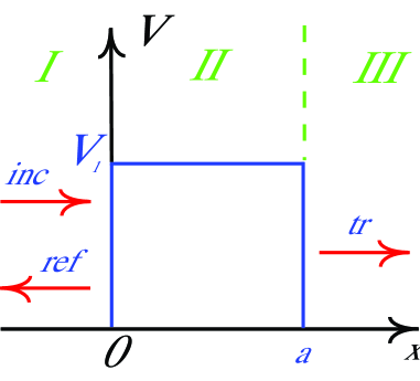
Figure 1: One-dimensional rectangular barrier

Let’s consider a problem of tunneling of a nonrelativistic particle in a positive $x$-dirrection through an one-dimensional rectangular potential barrier (see Fig. 1). Let’s label a region I for $x<0$, a region II for $0<x<a$ and a region III for $x>a$, accordingly. Let’s study an evolution of its tunneling through the barrier.

In a beginning we consider a standard approach to a solution of this problem [7, 8]. Let’s consider a case when levels of energy lay under than a height of the barrier: $E<V_{1}$.

The tunneling evolution of the particle can be described using a non-stationary consideration of a propagating w.p.

$$\psi(x,t)=\int\limits_{0}^{+\infty}g(E-\bar{E})\varphi(k,x)e^{-iEt/\hbar}dE,$$ (1)

where the stationary w.f. has a form:

$$\varphi(x)=\left\{\begin{array}[]{ll}e^{ikx}+A_{R}e^{-ikx},&\mbox{for }x<0;\\ \alpha e^{\xi x}+\beta e^{-\xi x},&\mbox{for }0<x<a;\\ A_{T}e^{ikx},&\mbox{for }x>a;\end{array}\right.$$ (2)

and $k=\frac{1}{\hbar}\sqrt{2mE}$, $\xi=\frac{1}{\hbar}\sqrt{2m(V_{1}-E)}$, $E$ and $m$ are the total energy and mass of the particle, accordingly. The weight amplitude $g(E-\bar{E})$ can be written in a form of gaussian [4] and satisfies to a requirement of the normalization $\int|g(E-\bar{E})|^{2}dE=1$, value $\bar{E}$ is an average energy of the particle. One can calculate coefficients $A_{T}$, $A_{R}$, $\alpha$ and $\beta$ analytically, using a requirements of a continuity of w.f. $\varphi(x)$ and its derivative on each boundary of the barrier.

Substituting in Eq. (1) instead of $\varphi(k,x)$ the incident $\varphi_{inc}(k,x)$, transmitted $\varphi_{tr}(k,x)$ or reflected part of w.f. $\varphi_{ref}(k,x)$, defined by Eq. (2), we receive the incident, transmitted or reflected w.p., accordingly.

We assume, that a time, for which the w.p. tunnels through the barrier, is enough small. So, the time necessary for a tunneling of an $\alpha$-parti le through a barrier of decay in $\alpha$-decay of a nucleus, is about $10^{-21}$ sekonds [9]. We consider, that one can neglect a spreading of the w.p. for this time. And a breadth of the w.p. appears essentially more narrow on a comparison with a barrier breadth [4, 5, 6]. Considering only sub-barrier processes, we exclude a component of waves for above-barrier energies, having included the additional transformation

$$g(E-\bar{E})\to g(E-\bar{E})\theta(V_{1}-E),$$ (3)

where $\theta$-function satisfies to the requirement

$$\theta(\eta)=\left\{\begin{array}[]{ll}0,&\mbox{for }\eta<0;\\ 1,&\mbox{for }\eta>0.\end{array}\right.$$

The method of multiple internal reflections considers the propagation process of the w.p. describing a motion of the particle, sequentially on steps of its penetration in relation to each boundary of the barrier [1, 2, 3]. Using this method, we find expressions for the transmitted and reflected w.p. in relation to the barrier.

At the first step we consider the w.p. in the region I, which is incident upon the first (initial) boundary of the barrier. Let’s assume, that this package transforms into the w.p., transmitted through this boundary and tunneling further in the region II, and into the w.p., reflected from the boundary and propagating back in the region I. Thus we consider, that the w.p., tunneling in the region II, is not reached the second (final) boundary of the barrier because of a terminating velocity of its propagation, and consequently at this step we consider only two regions I and II. Because of physical reasons to construct an expression for this packet, we consider, that its amplitude should decrease in a positive $x$-direction. We use only one item $\beta\exp(-\xi x)$ in Eq. (2), throwing the second increasing item $\alpha\exp(\xi x)$ (in an opposite case we break a requirement of a finiteness of the w.f. for an indefinitely wide barrier). In result, in the region II we obtain:

$$\psi^{1}_{tr}(x,t)=\int\limits_{0}^{+\infty}g(E-\bar{E})\theta(V_{1}-E)\beta^{0}e^{-\xi x-iEt/\hbar}dE,\mbox{for }0<x<a.$$ (4)

Thus the w.f. in the barrier region constructed by such way, is an analytic continuation of a relevant expression for the w.f., corresponding to a similar problem with above-barrier energies, where as a stationary expression we select the wave $\exp(ik_{2}x)$, propagated to the right.

Let’s consider the first step further. One can write expressions for the incident and the reflected w.p. in relation to the first boundary as follows

$$\begin{array}[]{lcll}\psi_{inc}(x,t)&=&\int\limits_{0}^{+\infty}g(E-\bar{E})\theta(V_{1}-E)e^{ikx-iEt/\hbar}dE,&\mbox{for }x<0,\\ \psi^{1}_{ref}(x,t)&=&\int\limits_{0}^{+\infty}g(E-\bar{E})\theta(V_{1}-E)A_{R}^{0}e^{-ikx-iEt/\hbar}dE,&\mbox{for }x<0.\end{array}$$ (5)

A sum of these expressions represents the complete w.f. in the region I, which is dependent on a time. Let’s require, that this w.f. and its derivative continuously transform into the w.f. (4) and its derivative at point $x=0$ (we assume, that the weight amplitude $g(E-\bar{E})$ differs weakly at transmitting and reflecting of the w.p. in relation to the barrier boundaries). In result, we obtain two equations, in which one can pass from the time-dependent w.p. to the corresponding stationary w.f. and obtain the unknown coefficients $\beta^{0}$ and $A_{R}^{0}$.

At the second step we consider the w.p., tunneling in the region II and incident upon the second boundary of the barrier at point $x=a$. It transforms into the w.p., transmitted through this boundary and propagated in the region III, and into the w.p., reflected from the boundary and tunneled back in the region II. For a determination of these packets one can use Eq. (1) with account (3), where as the stationary w.f. we use:

$$\begin{array}[]{lcll}\varphi_{inc}^{2}(k,x)&=&\varphi_{tr}^{1}(k,x)=\beta^{0}e^{-\xi x},&\mbox{for }0<x<a,\\ \varphi_{tr}^{2}(k,x)&=&A_{T}^{0}e^{ikx},&\mbox{for }x>a,\\ \varphi_{ref}^{2}(k,x)&=&\alpha^{0}e^{\xi x},&\mbox{for }0<x<a.\end{array}$$ (6)

Here, for forming an expression for the w.p. reflected from the boundary, we select an increasing part of the stationary solution $\alpha^{0}\exp(\xi x)$ only. Imposing a condition of continuity on the time-dependent w.f. and its derivative at point $x=a$, we obtain 2 new equations, from which we find the unknowns coefficients $A_{T}^{0}$ and $\alpha^{0}$.

At the third step the w.p., tunneling in the region II, is incident upon the first boundary of the barrier. Then it transforms into the w.p., transmitted through this boundary and propagated further in the region I, and into the w.p., reflected from boundary and tunneled back in the region II. For a determination of these packets one can use Eq. (1) with account Eq. (3), where as the stationary w.f. we use:

$$\begin{array}[]{lcll}\varphi_{inc}^{3}(k,x)&=&\varphi_{ref}^{2}(k,x),&\mbox{for }0<x<a,\\ \varphi_{tr}^{3}(k,x)&=&A_{R}^{1}e^{-ikx},&\mbox{for }x<0,\\ \varphi_{ref}^{3}(k,x)&=&\beta^{1}e^{-\xi x},&\mbox{for }0<x<a.\end{array}$$ (7)

Using a conditions of continuity for the time-dependent w.f. and its derivative at point $x=0$, we obtain the unknowns coefficients $A_{R}^{1}$ and $\beta^{1}$.

Analysing further possible processes of the transmission (and the reflection) of the w.p. through the boundaries of the barrier, we come to a deduction, that any of following steps can be reduced to one of 2 considered above. For the unknown coefficients $\alpha^{n}$, $\beta^{n}$,$A_{T}^{n}$ and $A_{R}^{n}$, used in expressions for the w.p., forming in result of some internal reflections from the boundaries, one can obtain the recurrence relations:

$$\begin{array}[]{lll}\beta^{0}=\displaystyle\frac{2k}{k+i\xi},&\alpha^{n}=\beta^{n}\displaystyle\frac{i\xi-k}{i\xi+k}e^{-2\xi a},&\beta^{n+1}=\alpha^{n}\displaystyle\frac{i\xi-k}{i\xi+k},\\ A_{R}^{0}=\displaystyle\frac{k-i\xi}{k+i\xi},&A_{T}^{n}=\beta^{n}\displaystyle\frac{2i\xi}{i\xi+k}e^{-\xi a-ika},&A_{R}^{n+1}=\alpha^{n}\displaystyle\frac{2i\xi}{i\xi+k}.\end{array}$$ (8)

Considering the propagation of the w.p. by such way, we obtain expressions for the w.f. on each region which can be written through series of multiple w.p.. Using Eq. (1) with account Eq. (3), we determine resultant expressions for the incident, transmitted and reflected w.p. in relation to the barrier, where one can need to use following expressions for the stationary w.f.:

$$\begin{array}[]{lcll}\varphi_{inc}(k,x)&=&e^{ikx},&\mbox{for }x<0,\\ \varphi_{tr}(k,x)&=&\sum\limits_{n=0}^{+\infty}A_{T}^{n}e^{ikx},&\mbox{for }x>a,\\ \varphi_{ref}(k,x)&=&\sum\limits_{n=0}^{+\infty}A_{R}^{n}e^{-ikx},&\mbox{for }x<0.\end{array}$$ (9)

Now we consider the w.p. formed in result of sequential $n$ reflections from the boundaries of the barrier and incident upon one of these boundaries at point $x=0$ ($i=1$) or at point $x=a$ ($i=2$). In result, this w.p. transforms into the w.p. $\psi_{tr}^{i}(x,t)$, transmitted through boundary with number $i$, and into the w.p. $\psi_{ref}^{i}(x,t)$, reflected from this boundary. For an independent on $x$ parts of the stationary w.f. one can write:

$$\begin{array}[]{ll}\displaystyle\frac{\varphi_{tr}^{1}}{\exp(-\xi x)}=T_{1}^{+}\displaystyle\frac{\varphi_{inc}^{1}}{\exp(ikx)},&\displaystyle\frac{\varphi_{ref}^{1}}{\exp(-ikx)}=R_{1}^{+}\displaystyle\frac{\varphi_{inc}^{1}}{\exp(ikx)},\\ \displaystyle\frac{\varphi_{tr}^{2}}{\exp(ikx)}=T_{2}^{+}\displaystyle\frac{\varphi_{inc}^{2}}{\exp(-\xi x)},&\displaystyle\frac{\varphi_{ref}^{2}}{\exp(\xi x)}=R_{2}^{+}\displaystyle\frac{\varphi_{inc}^{2}}{\exp(-\xi x)},\\ \displaystyle\frac{\varphi_{tr}^{1}}{\exp(-ikx)}=T_{1}^{-}\displaystyle\frac{\varphi_{inc}^{1}}{\exp(\xi x)},&\displaystyle\frac{\varphi_{ref}^{1}}{\exp(-\xi x)}=R_{1}^{-}\displaystyle\frac{\varphi_{inc}^{1}}{\exp(\xi x)},\end{array}$$ (10)

where the sign ”+” (or ”-”) corresponds to the w.p., tunneling (or propagating) in a positive (or negative) $x$-direction and incident upon the boundary with number $i$. Using $T_{i}^{\pm}$ and $R_{i}^{\pm}$, one can precisely describe an arbitrary w.p. which has formed in result of $n$-multiple reflections, if to know a “path” of its propagation along the barrier. Using the recurrence relations Eq. (8), the coefficients $T_{i}^{\pm}$ and $R_{i}^{\pm}$ can be obtained.

$$\begin{array}[]{lll}T_{1}^{+}=\beta^{0},&T_{2}^{+}=\displaystyle\frac{A_{T}^{n}}{\beta^{n}},&T_{1}^{-}=\displaystyle\frac{A_{R}^{n+1}}{\alpha^{n}},\\ R_{1}^{+}=A_{R}^{0},&R_{2}^{+}=\displaystyle\frac{\alpha^{n}}{\beta^{n}},&R_{1}^{-}=\displaystyle\frac{\beta^{n+1}}{\alpha^{n}}.\end{array}$$ (11)

Using the recurrence relations, one can find series of coefficients $\alpha^{n}$, $\beta^{n}$, $A_{T}^{n}$ and $A_{R}^{n}$. However, these series can be calculated easier, using coefficients $T_{i}^{\pm}$ and $R_{i}^{\pm}$. Analysing all possible “paths” of the w.p. propagations along the barrier, we receive:

$$\begin{array}[]{lcl}\sum\limits_{n=0}^{+\infty}A_{T}^{n}&=&T_{2}^{+}T_{1}^{-}\biggl{(}1+\sum\limits_{n=1}^{+\infty}(R_{2}^{+}R_{1}^{-})^{n}\biggr{)}=\displaystyle\frac{i4k\xi e^{-\xi a-ika}}{F_{sub}},\\ \sum\limits_{n=0}^{+\infty}A_{R}^{n}&=&R_{1}^{+}+T_{1}^{+}R_{2}^{+}T_{1}^{-}\biggl{(}1+\sum\limits_{n=1}^{+\infty}(R_{2}^{+}R_{1}^{-})^{n}\biggr{)}=\displaystyle\frac{k_{0}^{2}D_{-}}{F_{sub}},\\ \sum\limits_{n=0}^{+\infty}\alpha^{n}&=&\alpha^{0}\biggl{(}1+\sum\limits_{n=1}^{+\infty}(R_{2}^{+}R_{1}^{-})^{n}\biggr{)}=\displaystyle\frac{2k(i\xi-k)e^{-2\xi a}}{F_{sub}},\\ \sum\limits_{n=0}^{+\infty}\beta^{n}&=&\beta^{0}\biggl{(}1+\sum\limits_{i=1}^{+\infty}(R_{2}^{+}R_{1}^{-})^{n}\biggr{)}=\displaystyle\frac{2k(i\xi+k)}{F_{sub}},\\ \end{array}$$ (12)

where

$$\begin{array}[]{lll}F_{sub}&=&(k^{2}-\xi^{2})D_{-}+2ik\xi D_{+},\\ D_{\pm}&=&1\pm e^{-2\xi a},\\ k_{0}^{2}&=&k^{2}+\xi^{2}=\displaystyle\frac{2mV_{1}}{\hbar^{2}}.\end{array}$$ (13)

All series $\sum\alpha^{n}$, $\sum\beta^{n}$, $\sum A_{T}^{n}$ and $\sum A_{R}^{n}$, obtained using the method of multiple internal reflections, coincide with the corresponding coefficients $\alpha$, $\beta$, $A_{T}$ and $A_{R}$ of the Eq. (2), calculated by a stationary methods [4, 7, 10]. Using the following substitution

$$i\xi\to k_{2},$$ (14)

where $k_{2}=\frac{1}{\hbar}\sqrt{2m(E-V_{1})}$ is a wave number for a case of above-barrier energies, expression for the coefficients $\alpha^{n}$, $\beta^{n}$, $A_{T}^{n}$ and $A_{R}^{n}$ for each step, expressions for the w.f. for each step, the total Eqs. (12) and (13) transform into the corresponding expressions for a problem of the particle propagation above this barrier. At the transformation of the w.p. and the time-dependent w.f. one can need to change a sign of argument at $\theta$-function. Besides the following property is fulfilled:

$$\biggl{|}\sum\limits_{n=0}^{+\infty}A_{T}^{n}\biggr{|}^{2}+\biggl{|}\sum\limits_{n=0}^{+\infty}A_{R}^{n}\biggr{|}^{2}=1.$$ (15)

3 Tunneling of the particle through a spherically symmetric rectangular barrier

3.1 Transmitted and reflected wave packets

A problem of a motion of two interacting particles can be redused to a problem of one particle scattering in a spherically symmetric field. Let’s assume, that the particle under an action of a central force

$$V(r)=\left\{\begin{array}[]{rll}-V_{0},&\mbox{for }r<R_{1};&\mbox{(region I)};\\ V_{1},&\mbox{for }R_{1}<r<R_{2},&\mbox{(region II)};\\ 0,&\mbox{for }r>R_{2},&\mbox{(region III)}.\end{array}\right.$$ (16)

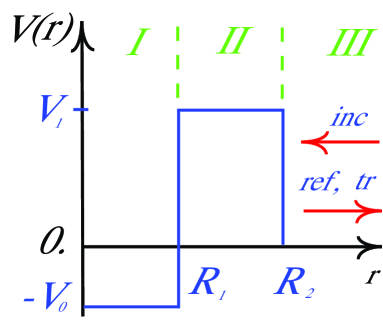
Figure 2: Spherically symmetric rectangular barrier

is incident outside upon an external boundary of the barrier at point $r=R_{2}$ (see Fig. 2).

Let’s study an evolution of tunneling of the particle through the barrier. We consider a case when the moment $l=0$ and levels of energy lay below than a barrier height. The tunneling evolution of the particle in time dependence can be described using a w.p. constructed on a basis of a stationary solution of the following form [7]:

$$\psi(r,\theta,\varphi)=\frac{\chi(r)}{r}Y_{lm}(\theta,\varphi),$$ (17)

$$\chi(r)=\left\{\begin{array}[]{lll}A(e^{-ik_{1}r}-e^{ik_{1}r}),&\mbox{for }r<R_{1},&\mbox{(region I)},\\ \alpha e^{\xi r}+\beta e^{-\xi r},&\mbox{for }R_{1}<r<R_{2},&\mbox{(region II)},\\ e^{-ikr}+Se^{ikr},&\mbox{for }r>R_{2},&\mbox{(region III)},\end{array}\right.$$ (18)

where $Y_{lm}(\theta,\varphi)$ is a spherical function, $k_{1}=\frac{1}{\hbar}\sqrt{2m(E+V_{0})}$, $\xi=\frac{1}{\hbar}\sqrt{2m(V_{1}-E)}$, $k=\frac{1}{\hbar}\sqrt{2mE}$. For the spherically symmetric problem in a case of sub-barrier energies we obtain:

$$\chi(r,t)=\int\limits_{0}^{+\infty}g(E-\bar{E})\theta(V_{l}-E)\chi(k,r)e^{-iEt/\hbar}dE,$$ (19)

$$V_{l}(r)=V(r)+\displaystyle\frac{\hbar^{2}}{2m}\displaystyle\frac{l(l+1)}{r^{2}},$$ (20)

where the second item in Eq. (20) is a centrifugal energy, which is equal to zero at $l=0$, weight amplitude $g(E-\bar{E})$ and average energy of the particle $\bar{E}$ are defined similarly to the one-dimensional problem (see Sec. 2).

At a stationary consideration of the solutions (18) we describe the particle incident upon the external boundary of the barrier by a spherical wave $\exp(-ikr)$ convergent to the centre. And we describe the particle scattered on the barrier in the region III by a spherical wave $S\exp(ikr)$ divergent outside. The scattered wave takes into account both a possibility of a reflection of the particle from the barrier, which is written by the divergent wave, and a possibility of a penetration of the particle through the barrier, when in a beginning the particle tunnels from the region III to the region I, and then after some period of time it tunnels back from the region I to the region III and also is written by the divergent wave. Only one item $S\exp(ikr)$ contains the transmitted and reflected divergent waves, and it is impossible to separate them at the stationary consideration.

As non-stationary, the method of multiple internal reflections allows to find a solution of this problem. Let’s apply it to this problem. We study a propagation of a w.p. describing tunneling of the particle, sequentially on steps of its transmission in relation to each of boundaries of the barrier (similarly to the one-dimensional problem). In result of an analysis we come to a deduction, that any step in such viewing of the propagation of the w.p. along the barrier will be similar to one of 4 steps independent among themselves. Analysing these 4 steps further, one can obtain recurrence relations for finding coefficients $A^{n}$, $S^{n}$, $\alpha^{n}$ and $\beta^{n}$ for an arbitrary step $n$.

In result of multiple internal reflections (and transitions) in relation to the boundaries of the barrier a total time-dependent w.f. in each region can be written in a form of series, composed from convergent and divergent w.p.. Analysing possible “paths” of propagations of these packets, one can calculate expressions for series of coefficients $S^{n}$, $A^{n}$, $\alpha^{n}$ and $\beta^{n}$:

$$\begin{array}[]{lcl}\sum\limits_{n=1}^{+\infty}S^{n}&=&\displaystyle\frac{1}{F_{sub}}T_{2}^{-}T_{2}^{+}(R_{1}^{-}(1-R_{1}^{+}R_{0}^{-})+T_{1}^{-}R_{0}^{-}T_{1}^{+})=\\ &=&\displaystyle\frac{4ik\xi\biggl{(}\displaystyle\frac{i\xi-k_{1}}{i\xi+k_{1}}-e^{2ik_{1}R_{1}}\biggr{)}e^{2\xi(R_{1}-R_{2})-2ikR_{2}}}{F_{sub}(k+i\xi)^{2}},\\ \sum\limits_{n=0}^{+\infty}A^{n}&=&\displaystyle\frac{T_{1}^{-}T_{2}^{-}}{F_{sub}}=\displaystyle\frac{4ik\xi e^{-ikR_{2}+ik_{1}R_{1}-\xi(R_{2}-R_{1})}}{F_{sub}(k+i\xi)(k_{1}+i\xi)},\\ \sum\limits_{n=0}^{+\infty}\alpha^{n}&=&\alpha^{0}\displaystyle\frac{1-R_{1}^{+}R_{0}^{-}}{F_{sub}}=\displaystyle\frac{2k\biggl{(}1+\displaystyle\frac{k_{1}-i\xi}{k_{1}+i\xi}e^{2ik_{1}R_{1}}\biggr{)}e^{-(\xi+ik)R_{2}}}{F_{sub}(k+i\xi)},\\ \sum\limits_{n=0}^{+\infty}\beta^{n}&=&\displaystyle\frac{\sum\limits_{n=0}^{+\infty}\alpha^{n}-T_{2}^{-}}{R_{2}^{+}}=\alpha^{0}\displaystyle\frac{R_{1}^{-}(1-R_{1}^{+}R_{0}^{-})+T_{1}^{-}R_{0}^{-}T_{1}^{+}}{F_{sub}}=\\ &=&\displaystyle\frac{2k\biggl{(}\displaystyle\frac{i\xi-k_{1}}{i\xi+k_{1}}-e^{2ik_{1}R_{1}}\biggr{)}e^{\xi(2R_{1}-R_{2})-ikR_{2}}}{F_{sub}(k+i\xi)},\end{array}$$ (21)

where

$$\begin{array}[]{lcl}F_{sub}&=&(1-R_{1}^{+}R_{0}^{-})(1-R_{2}^{+}R_{1}^{-})-R_{2}^{+}T_{1}^{-}R_{0}^{-}T_{1}^{+}=1+\displaystyle\frac{k_{1}-i\xi}{k_{1}+i\xi}e^{2ik_{1}R_{1}}-\\ &-&\displaystyle\frac{(k-i\xi)(k_{1}-i\xi)}{(k+i\xi)(k_{1}+i\xi)}e^{-2\xi(R_{2}-R_{1})}-\displaystyle\frac{k-i\xi}{k+i\xi}e^{-2\xi(R_{2}-R_{1})+2ik_{1}R_{1}}.\end{array}$$ (22)

$$\begin{array}[]{ll}T_{2}^{-}=\alpha^{0}=\displaystyle\frac{2k}{k+i\xi}e^{-(\xi+ik)R_{2}},&R_{2}^{-}=S^{0}=\displaystyle\frac{-i\xi+k}{i\xi+k}e^{-2ikR_{2}},\\ T_{1}^{-}=\displaystyle\frac{A^{n}}{\alpha^{n}}=\displaystyle\frac{2i\xi}{i\xi+k_{1}}e^{(\xi+ik_{1})R_{1}},&R_{1}^{-}=\displaystyle\frac{\beta^{n}}{\alpha^{n}}=\displaystyle\frac{i\xi-k_{1}}{i\xi+k_{1}}e^{2\xi R_{1}},\\ T_{0}^{-}=0,&R_{0}^{-}=1,\\ T_{1}^{+}=\displaystyle\frac{\beta^{n+1}}{A^{n}}=-\displaystyle\frac{2k_{1}}{i\xi+k_{1}}e^{(\xi+ik_{1})R_{1}},&R_{1}^{+}=\displaystyle\frac{A^{n+1}}{A^{n}}=\displaystyle\frac{i\xi-k_{1}}{i\xi+k_{1}}e^{2ik_{1}R_{1}},\\ T_{2}^{+}=\displaystyle\frac{S^{n+1}}{\beta^{n}}=\displaystyle\frac{2i\xi}{i\xi+k}e^{-(\xi+ik)R_{2}},&R_{2}^{+}=\displaystyle\frac{\alpha^{n+1}}{\beta^{n}}=\displaystyle\frac{i\xi-k}{i\xi+k}e^{-2\xi R_{2}},\end{array}$$ (23)

where the coefficients $T_{i}^{\pm}$ and $R_{i}^{\pm}$ are defined in relation to the boundary with number $i$ ($i=0$ for $r=0$, $i=1$ for $r=R_{1}$ and $i=2$ for $r=R_{2}$). They can be calculated using of the recurrence relations between the coefficients $S^{n}$, $A^{n}$, $\alpha^{n}$ and $\beta^{n}$.

Now we consider the incident, transmitted and reflected w.p. in relation to the barrier as a whole. Defining them for the region III, one can write:

$$\begin{array}[]{lcl}\chi_{inc}(r,t)&=&\int\limits_{0}^{+\infty}g(E-\bar{E})\theta(V_{1}-E)e^{-ikr-iEt/\hbar}dE,\\ \chi_{tr}(r,t)&=&\int\limits_{0}^{+\infty}g(E-\bar{E})\theta(V_{1}-E)S_{tr}e^{ikr-iEt/\hbar}dE,\\ \chi_{ref}(r,t)&=&\int\limits_{0}^{+\infty}g(E-\bar{E})\theta(V_{1}-E)S_{ref}e^{ikr-iEt/\hbar}dE,\end{array}$$ (24)

where

$$\begin{array}[]{lcl}S_{tr}&=&\sum\limits_{n=1}^{+\infty}S^{n},\\ S_{ref}&=&S^{0},\\ S&=&S_{tr}+S_{ref}.\end{array}$$ (25)

The expression $S$ represents a diagonal element of scattering matrix corresponding to the orbital moment $l=0$. Thus, using the method of multiple internal reflections it appears possible to divide the S-matrix into two components corresponding to amplitudes of stationary parts of the transmitted and reflected w.p. in relation to the barrier as a whole. This property having physical sense, is obtained for the first time.

The expressions for coefficients $S^{n}$, $A^{n}$, $\alpha^{n}$ and $\beta^{n}$ for each step, the expression for the w.f. for each step, the coefficients $T_{i}^{\pm}$ and $R_{i}^{\pm}$, the series of the coefficients $S^{n}$, $A^{n}$, $\alpha^{n}$ and $\beta^{n}$ under the substitution (14) (and also at replacement of a sign before argument for $\theta$-function at a consideration of the non-stationary w.p.) transform into the corresponding expressions for a solution of a problem of a w.p. propagation above the barrier. The series (21) of the coefficients $S^{n}$, $A^{n}$, $\alpha^{n}$ and $\beta^{n}$ coincide with the corresponding coefficients $S$, $A$, $\alpha$ and $\beta$ for Eq. (18), calculated by stationary methods.

3.2 Tunneling and reflecting times in relation to the barrier

One can determine an equation for a propagation of a maximum of the incident, transmitted and reflected w.p. in relation to the barrier for the spherically symmetric problem. For radial parts of non-stationary w.f. one can write:

$$\frac{\partial}{\partial E}\mbox{arg }\chi_{inc}(r,t)=\displaystyle\frac{\partial}{\partial E}\mbox{arg }\chi_{tr}(r,t)=\displaystyle\frac{\partial}{\partial E}\mbox{arg }\chi_{ref}(r,t)=const.$$ (26)

Let’s consider the first step of the propagation of the w.p.. Let the w.p. is incident in the region III upon the external boundary of the barrier at point $r=R_{2}$ in a time moment $t_{inc}$. Using Eq. (26), we find the time moment $t_{ref}^{1}$ of leaving outside from this boundary the reflected w.p. in the region III:

$$t_{ref}^{1}=t_{inc}+\displaystyle\frac{2mR_{2}}{\hbar k}+\hbar\displaystyle\frac{\partial\mbox{arg }S^{0}}{\partial E}.$$ (27)

Similarly, for a time moment $t_{tr}^{n}$ of leaving outside from the external boundary of the barrier the $n$-multiple transmitted w.p. one can write:

$$t_{tr}^{n}=t_{inc}+\displaystyle\frac{2mR_{2}}{\hbar k}+\hbar\displaystyle\frac{\partial\mbox{arg }S^{n}}{\partial E}.$$ (28)

Using Eq. (26) at point $r=R_{2}$, we find times necessary for the penetration of the total w.p. through the barrier (describing the tunneling of the particle through the barrier) and for the reflection of the w.p. from the barrier (describing the reflection of the particle from the barrier):

$$\begin{array}[]{lcl}\tau_{tun}^{Ph}&=&t_{tr}-t_{inc}=\displaystyle\frac{2mR_{2}}{\hbar k}+\hbar\displaystyle\frac{\partial\mbox{arg }S_{tr}}{\partial E},\\ \tau_{ref}^{Ph}&=&t_{ref}-t_{inc}=\displaystyle\frac{2mR_{2}}{\hbar k}+\hbar\displaystyle\frac{\partial\mbox{arg }S_{ref}}{\partial E}.\end{array}$$ (29)

For the problem of the w.p. tunneling under the barrier we receive:

$$\begin{array}[]{lcl}\tau_{tun}^{Ph}&=&\hbar\displaystyle\frac{\partial}{\partial E}\mbox{arg }\displaystyle\frac{i\xi-k_{1}-(i\xi+k_{1})e^{2ik_{1}R_{1}}}{(i\xi+k)^{2}(i\xi+k_{1})F_{sub}},\\ \tau_{ref}^{Ph}&=&\displaystyle\frac{2m}{\hbar\xi k}.\end{array}$$ (30)

For the problem of the w.p. propagating above the barrier we write:

$$\begin{array}[]{lcl}\tau_{tun}^{Ph}&=&\displaystyle\frac{2m(R_{2}-R_{1})}{\hbar k_{2}}+\hbar\displaystyle\frac{\partial}{\partial E}\mbox{arg }\displaystyle\frac{k_{2}-k_{1}-(k_{2}+k_{1})e^{2ik_{1}R_{1}}}{(k+k_{2})(k_{1}+k_{2})F_{above}},\\ \tau_{ref}^{Ph}&=&0,\end{array}$$ (31)

where $F_{above}$ can be obtained from $F_{sub}$ using the substitution (14).

Let’s consider a particle, which tunnels under a high enough and wide barrier. Then for the time of the tunneling we obtain the following expression (sequence of approaches: $\xi(R_{2}-R_{1})\to+\infty$, $\xi\to+\infty$, $R_{2}-R_{1}\to+\infty$):

$$\tau_{tun}^{Ph}=\displaystyle\frac{2m}{\hbar k\xi}+\displaystyle\frac{4mR_{1}\sin{2k_{1}R_{1}}(1-2\cos{2k_{1}R_{1}})}{\hbar\xi(1-\cos{2k_{1}R_{1}})}.$$ (32)

The tunneling time does not depend on a width of the barrier (Hartman’s and Fletcher’s effect), but depends on $k_{1}$ and $R_{1}$.

4 Tunneling of the particle through the spherically symmetric barrier of a general view

4.1 The particle propagates above the barrier

In study of nuclear processes when a tunneling of parti les through a barrier is investigated, in the most cases the barriers of more complicated form than rectangular are used. So, the spherically symmetric two-humb potential of Strutinski has an enough important role in problems of fission and decai of nuclei. A degree of an exactitude of a description of the nuclear process depends on choice of a form of the potential. Therefore, we shall consider, as far as it is possible to use the method of multiple internal reflections for solving the spherically symmetrical problems with the barrier of a general view.

Let’s consider a particle propagating in a spherically symmetric potential field, which radial part has a barrier. Taking into account a behaviour of a radial part $V(r)$ of the potential function in dependence on $r$, we divide the area of its definition $r\in[0;+\infty[$ on $n$ regions. In each region let’s replace the potential function $V(r)$ by a function most close describing $V(r)$ and for which an exact solution of the stationary Schrödinger equation exists (see Fig. LABEL:fig4). Passing to the problem of the particle propagation in the field of these approximated potential functions, we write the general solution for stationary w.f. in the form (17), where its radial part can be written as

$$\chi(r)=\left\{\begin{array}[]{lll}A_{1}a_{1}(k,r)+B_{1}b_{1}(k,r),&\mbox{for }0<r<R_{1},&\mbox{(region I)},\\ A_{i}a_{i}(k,r)+B_{i}b_{i}(k,r),&\mbox{for }R_{i-1}<r<R_{i},&\mbox{(region i)},\\ A_{n}a_{n}(k,r)+B_{n}b_{n}(k,r),&\mbox{for }r>R_{n-1},&\mbox{(region N)},\end{array}\right.$$ (33)

where $k=\frac{1}{\hbar}\sqrt{2mE}$, $a_{i}(k,r)$ and $b_{i}(k,r)$ are the partial solutions of the radial part of w.f. in region $i$, $A_{i}$ and $B_{i}$ are the normalization constants.

Let’s find the transmission and reflection coefficients of particle in relation to the barrier, and also the times necessary for transmission and for reflection of the particle in relation to the barrier, using the method of multiple internal reflections. To apply the method to this problem, one can need to present the general stationary solution of w.f. in each region in the sum of divergent and convergent vawes.

Using the Fourier transformation, one can write:

$$\begin{array}[]{lcl}a_{i}(k,r)&=&a_{i}^{-}(k,r)+a_{i}^{+}(k,r),\\ b_{i}(k,r)&=&b_{i}^{-}(k,r)+b_{i}^{+}(k,r),\end{array}$$ (34)

where

$$\begin{array}[]{lcl}a_{i}^{-}(k,r)&=&\displaystyle\frac{1}{\sqrt{2\pi}}\int\limits_{-\infty}^{0}dq\int\limits_{R_{i-1}}^{R_{i}}a_{i}(k,r^{\prime})e^{iq(r-r^{\prime})}dr^{\prime},\\ a_{i}^{+}(k,r)&=&\displaystyle\frac{1}{\sqrt{2\pi}}\int\limits_{0}^{+\infty}dq\int\limits_{R_{i-1}}^{R_{i}}a(k,r^{\prime})e^{iq(r-r^{\prime})}dr^{\prime},\\ b_{i}^{-}(k,r)&=&\displaystyle\frac{1}{\sqrt{2\pi}}\int\limits_{-\infty}^{0}dq\int\limits_{R_{i-1}}^{R_{i}}b_{i}(k,r^{\prime})e^{iq(r-r^{\prime})}dr^{\prime},\\ b_{i}^{+}(k,r)&=&\displaystyle\frac{1}{\sqrt{2\pi}}\int\limits_{0}^{+\infty}dq\int\limits_{R_{i-1}}^{R_{i}}b_{i}(k,r^{\prime})e^{iq(r-r^{\prime})}dr^{\prime}.\end{array}$$ (35)

Taking into account the transformation

$$\begin{array}[]{lcl}c_{i}^{-}(k,r)&=&a_{i}^{-}(k,r)+\displaystyle\frac{B_{i}}{A_{i}}b_{i}^{-}(k,r),\\ c_{i}^{+}(k,r)&=&\displaystyle\frac{A_{i}}{B_{i}}a_{i}^{+}(k,r)+b_{i}^{+}(k,r)\end{array}$$ (36)

one can write the general solusion (33) as

$$\chi(r)=\left\{\begin{array}[]{lll}A_{1}c_{1}^{-}(k,r)+B_{1}c_{1}^{+}(k,r),&\mbox{for }0<r<R_{1},&\mbox{(region I)},\\ A_{i}c_{i}^{-}(k,r)+B_{i}c_{i}^{+}(k,r),&\mbox{for }R_{i-1}<r<R_{i},&\mbox{(region i)},\\ A_{n}c_{n}^{-}(k,r)+B_{n}c_{n}^{+}(k,r),&\mbox{for }r>R_{n-1},&\mbox{(region N)},\end{array}\right.$$ (37)

In result, the general solution in every region $i$ is represented as the sum of convergent vawes $c_{i}^{-}(r)$ and divergent vawes $c_{i}^{+}(r)$ (so, in case of a rectangular barrier in the region $i$ such expressions equal to $e^{-ik_{i}r}$ and $e^{ik_{i}r}$, accordingly). On the basis of these expressions using Eq. (19) one can construct the non-stationary convergent and divergent w.p.. Writing the genegal solution for w.f. in every region in the form of linear combination of convergent and divergent w.p., one can apply the method of multiple internal reflections for solving the problem.

At first we study the case, when the general stationary solution for w.f. in every region can be written uniquely as sum of convergent and divergent vawes $c_{i}^{\pm}(r)$. Then using of the method of multiple internal reflections for solving the problem, one can find the incident, transmitted and reflected w.p. in relation to the barrier at whole, and total w.p. in every region. It is enough convenient to use the coefficients $T_{i}^{\pm}$ and $R_{i}^{\pm}$ (as in the spherically symmetric problem with rectangular barrier). We define these coefficients in relation to the boundary with the number $i$ by such way (for the step $j$):

$$\begin{array}[]{lcllcl}A_{i}^{j}&=&T_{i}^{-}A_{i+1}^{j};&B_{i+1}^{j+1}&=&R_{i}^{-}A_{i+1}^{j};\\ B_{i+1}^{j}&=&T_{i}^{+}B_{i}^{j};&A_{i}^{j+1}&=&R_{i}^{+}B_{i}^{j}.\end{array}$$ (38)

One can calculate these coefficients at consideration of first $2n+1$ steps:

$$\begin{array}[]{ll}T_{0}^{-}=0;&R_{0}^{-}=-\displaystyle\frac{c_{1}^{-}(0)}{c_{1}^{+}(0)}=\displaystyle\frac{B_{1}}{A_{1}},\end{array}$$ (39)

$$\begin{array}[]{lcl}T_{i}^{-}&=&\displaystyle\frac{\displaystyle\frac{\partial c_{i+1}^{-}(r)}{\partial r}c_{i+1}^{+}(r)-c_{i+1}^{-}(r)\displaystyle\frac{\partial c_{i+1}^{+}(r)}{\partial r}}{\displaystyle\frac{\partial c_{i}^{-}(r)}{\partial r}c_{i+1}^{+}(r)-c_{i}^{-}(r)\displaystyle\frac{\partial c_{i+1}^{+}(r)}{\partial r}}\Biggl{|}_{r=R_{i}},\\ R_{i}^{-}&=&\displaystyle\frac{\displaystyle\frac{\partial c_{i+1}^{-}(r)}{\partial r}c_{i}^{-}(r)-c_{i+1}^{-}(r)\displaystyle\frac{\partial c_{i}^{-}(r)}{\partial r}}{\displaystyle\frac{\partial c_{i}^{-}(r)}{\partial r}c_{i+1}^{+}(r)-c_{i}^{-}(r)\displaystyle\frac{\partial c_{i+1}^{+}(r)}{\partial r}}\Biggl{|}_{r=R_{i}},\\ T_{i}^{+}&=&\displaystyle\frac{\displaystyle\frac{\partial c_{i}^{+}(r)}{\partial r}c_{i}^{-}(r)-c_{i}^{+}(r)\displaystyle\frac{\partial c_{i+1}^{-}(r)}{\partial r}}{\displaystyle\frac{\partial c_{i+1}^{+}(r)}{\partial r}c_{i}^{-}(r)-c_{i+1}^{+}(r)\displaystyle\frac{\partial c_{i}^{-}(r)}{\partial r}}\Biggl{|}_{r=R_{i}},\\ R_{i}^{+}&=&\displaystyle\frac{\displaystyle\frac{\partial c_{i}^{+}(r)}{\partial r}c_{i+1}^{+}(r)-c_{i}^{+}(r)\displaystyle\frac{\partial c_{i+1}^{-}(r)}{\partial r}}{\displaystyle\frac{\partial c_{i+1}^{+}(r)}{\partial r}c_{i+1}^{+}(r)-c_{i+1}^{+}(r)\displaystyle\frac{\partial c_{i}^{-}(r)}{\partial r}}\Biggl{|}_{r=R_{i}}.\end{array}$$ (40)

Further using the method of multiple internal reflections, one can calculate the incident, transmitted and reflected w.p. in relation to the barrier. On the basis of these w.p. one can find the transmission and reflection coefficients and also the transmission and reflection times in relation to the barrier. Thus the transmitted and reflected w.p. can be written through $S_{tr}$ and $S_{ref}$, which sum is the diagonal element of the scattering matrix $S$ at the orbital moment $l$.

The value $A_{n}$ can be obtained from the normalization condition:

$$A_{n}=\Biggl{(}\int\limits_{R_{n-1}}^{+\infty}|c_{n}(k,r)|^{2}dr\Biggr{)}^{-1/2}.$$ (41)

Now we study the case, when the partial solutions of w.f. in some regions are not the convergent and divergent vawes. In representations (36) and (37) one can need to know the values $B_{i}/A_{i}$. In this case at solving the problem we consider first $2n+1$ steps. Let the general solution for w.f. in first region be expressed through $a_{1}$ and $b_{1}$. Analyzing the reflection of w.p. from point $r=0$, one can obtain:

$$\begin{array}[]{ll}T_{0}^{-}=0;&R_{0}^{-}=-\displaystyle\frac{a_{1}(0)}{b_{1}(0)}=\displaystyle\frac{B_{1}}{A_{1}}.\end{array}$$ (42)

If the w.f. in the first region is determined through $c_{1}^{\pm}$ uniquely, then it is need to use Eq. (39) instead of Eq. (42). Calculating the value $B_{1}/A_{1}$, then one can find the functions $c_{1}^{\pm}$. Using the continuity condition for w.f. and its derivative in all boundaries between regions, one can find the recurrent relation for values $B_{i}/A_{i}$:

$$\begin{array}[]{l}\displaystyle\frac{B_{i+1}}{A_{i+1}}=\displaystyle\frac{f_{i}(r)\displaystyle\frac{\partial a_{i+1}(r)}{\partial r}-\displaystyle\frac{\partial f_{i}(r)}{\partial r}a_{i+1}(r)}{\displaystyle\frac{\partial f_{i}(r)}{\partial r}b_{i+1}(r)-f_{i}(r)\displaystyle\frac{\partial b_{i+1}(r)}{\partial r}}\Biggl{|}_{r=R_{i}},\\ f_{i}(r)=a_{i}(r)+b_{i}(r)\displaystyle\frac{B_{i}}{A_{i}}\Biggl{|}_{r=R_{i}}=c_{i}^{-}(r)+c_{i}^{+}\displaystyle\frac{B_{i}}{A_{i}}\Biggl{|}_{r=R_{i}}.\end{array}$$ (43)

Having the values $B_{i}/A_{i}$, we obtain the convergent and divergent vawes $c_{i}^{\pm}(r)$ in every region. Then the solution of problem is fulfilled as in the previous case.

Applying the approach considered above for the solution of problem of particle propagation, when the potential $V(r)$ is defined only in two regions ($n=2$), one can find the incident, transmitted and reflected w.p. in relation to the barrier using Eq. (19) for above-barrier region, where the radial parts from corresponding stationary w.f. have the form (at $r>R_{1}$)

$$\begin{array}[]{lcll}\chi_{inc}(r)&=&A_{2}c_{2}^{-}(k,r),\\ \chi_{tr}(r)&=&S_{tr}c_{2}^{+}(k,r)=A_{2}\displaystyle\frac{T_{1}^{-}T_{1}^{+}R_{0}^{-}}{1-R_{1}^{+}R_{0}^{-}}c_{2}^{+}(k,r),\\ \chi_{ref}(r)&=&S_{ref}c_{2}^{+}(k,r)=A_{2}R_{1}^{-}c_{2}^{+}(k,r).\end{array}$$ (44)

We find the coefficients $T_{i}^{\pm}$ and $R_{i}^{\pm}$ from Eq. (40). Using Eq. (26) for external boundary, one can obtain the times necessary for transmission and for reflection of particle in relation to the barrier. In result, we receive:

$$\begin{array}[]{lcl}\tau_{tun}&=&\hbar\displaystyle\frac{\partial}{\partial E}\Biggl{(}\mbox{arg }\biggl{(}\sum\limits_{n=1}^{+\infty}B_{2}^{i}c_{2}^{+}(k,R_{1})\biggr{)}-\mbox{arg }A_{2}c_{2}^{-}(k,R_{1})\Biggr{)}=\\ &=&\hbar\displaystyle\frac{\partial}{\partial E}\mbox{arg }\displaystyle\frac{T_{1}^{-}T_{1}^{+}R_{0}^{-}}{1-R_{1}^{+}R_{0}^{-}}+\Delta\tau;\\ \tau_{ref}&=&\hbar\displaystyle\frac{\partial}{\partial E}\Biggl{(}\mbox{arg }\biggl{(}B_{2}^{0}c_{2}^{+}(k,R_{1})\biggr{)}-\mbox{arg }A_{2}c_{2}^{-}(k,R_{1})\Biggr{)}=\\ &=&\hbar\displaystyle\frac{\partial}{\partial E}\mbox{arg }R_{1}^{-}+\Delta\tau;\\ \Delta\tau&=&\hbar\displaystyle\frac{\partial}{\partial E}\mbox{arg }\displaystyle\frac{c_{2}^{+}(R_{1})}{c_{2}^{-}(R_{1})}.\end{array}$$ (45)

For the problem solution when potential $V(r)$ is defined on three regions ($n=3$), the expressions for radial parts of stationary w.f., describing the incident, transmitted and reflected w.p. in relation to the barrier, look like (at $r>R_{2}$)

$$\begin{array}[]{lcll}\chi_{inc}(r)&=&A_{3}c_{3}^{-}(k,r),\\ \chi_{tr}(r)&=&S_{tr}c_{3}^{+}(k,r)=A_{3}\displaystyle\frac{T_{2}^{-}T_{2}^{+}(R_{1}^{-}(1-R_{1}^{+}R_{0}^{-})+T_{1}^{-}R_{0}^{-}T_{1}^{+})}{(1-R_{1}^{+}R_{0}^{-})(1-R_{2}^{+}R_{1}^{-})-R_{2}^{+}T_{1}^{-}R_{0}^{-}T_{1}^{+}}c_{3}^{+}(k,r)\\ \chi_{ref}(r)&=&S_{ref}c_{3}^{+}(k,r)=A_{3}R_{2}^{-}c_{3}^{+}(k,r).\end{array}$$ (46)

The transmission and reflection times of particle in relation to the barrier has the form (they are calculated at $r=R_{2}$)

$$\begin{array}[]{lcl}\tau_{tun}&=&\hbar\displaystyle\frac{\partial}{\partial E}\mbox{arg }\displaystyle\frac{T_{2}^{-}T_{2}^{+}(R_{1}^{-}(1-R_{1}^{+}R_{0}^{-})+T_{1}^{-}R_{0}^{-}T_{1}^{+})}{(1-R_{1}^{+}R_{0}^{-})(1-R_{2}^{+}R_{1}^{-})-R_{2}^{+}T_{1}^{-}R_{0}^{-}T_{1}^{+}}+\Delta\tau;\\ \tau_{ref}&=&\hbar\displaystyle\frac{\partial}{\partial E}\mbox{arg }R_{2}^{-}+\Delta\tau;\\ \Delta\tau&=&\hbar\displaystyle\frac{\partial}{\partial E}\mbox{arg }\displaystyle\frac{c_{3}^{+}(R_{2})}{c_{3}^{-}(R_{2})}.\end{array}$$ (47)

As an examples of method application we consider two problems.

The particle propagates above the barrier of form (see Fig. LABEL:fig5)

$$V(r)=\left\{\begin{array}[]{cll}-V_{0},&\mbox{for }0<r<R_{1},&\mbox{(region I)};\\ \displaystyle\frac{\gamma}{r},&\mbox{for }r>R_{1},&\mbox{(region II)}.\end{array}\right.$$ (48)

We consider the case $l\neq 0$. One can obtain the incident, transmitted and reflected w.p. in relation to the barrier from Eqs. (44) and (19), taking into account the sign before argument of $\theta$-function for above-barrier energies, and transmission and reflection times from Eq. (45). At consideration the first three steps of w.p. propagation along the barrier we find the coefficients $T_{i}^{\pm}$ and $R_{i}^{\pm}$ using Eqs. (40) for $n=2$. In the solutions one can need to fulfil the substitution

$$\begin{array}[]{lcllcl}c_{1}^{-}(k,r)&=&\chi_{k_{1}l}^{-}(r),&c_{2}^{-}(k,r)&=&G_{l}(\eta,\rho)-iF_{l}(\eta,\rho),\\ c_{1}^{+}(k,r)&=&\chi_{k_{1}l}^{+}(r),&c_{2}^{+}(k,r)&=&G_{l}(\eta,\rho)+iF_{l}(\eta,\rho),\end{array}$$ (49)

where

$$\begin{array}[]{lcllcl}k_{1}&=&\frac{1}{\hbar}\sqrt{2m(E+V_{0})},\\ \eta&=&\displaystyle\frac{\mu\nu k}{\hbar^{2}},\\ \rho&=&k(r),\\ \chi_{k_{1}l}^{\pm}(r)&=&\pm i\sqrt{\displaystyle\frac{\pi k_{1}r}{2}}H_{l+1/2}^{(1,2)}(k_{1}r),\end{array}$$ (50)

$H_{l}^{(1,2)}(r)$ is the function of Hankel of 1-st and 2 sort,
$G_{l}(\eta,\rho)$ and $F_{l}(\eta,\rho)$ are the irregular and regular Coulomb functions [11]. The normalization constant $A_{2}$ can be obtained from Eq. (41).

Now we consider another problem when the particle propagates above the barrier of following form:

$$V(r)=\left\{\begin{array}[]{cll}\alpha r^{2}-V_{0},&\mbox{for }0<r<R_{1},&\mbox{(region I)};\\ \displaystyle\frac{\gamma}{r},&\mbox{for }r>R_{1},&\mbox{(region II)}.\end{array}\right.$$ (51)

Let’s study the case $l=0$. In the beginning we consider region I. The partial solutions for the radial part of stationary w.f. are the parabolic cylinder functions [11]: $D_{\nu}(\pm gr)$ and $D_{\nu}(\pm igr)$, where $g=(8\alpha\mu/\hbar^{2})^{1/4}$. For the description of above-barrier motion of particle we choose the first two solutions $D_{\nu}(\pm gr)$, which are independent if $\nu$ is non-integer. (Note that one can use the Whitteker’s functions as such two independent solutions [11]. But these two functions can be presented in the form of linear combination of the parabolic cylinder functions $D_{\nu}(\pm gr)$.) Each of partial solutions can be presented in the form of sum of convergent and divergent waves:

$$\begin{array}[]{lcl}D_{\nu}(\pm gr)&=&D_{\nu}^{-}(\pm gr)+D_{\nu}^{+}(\pm gr),\\ D_{\nu}(\pm gr)^{-}&=&\displaystyle\frac{1}{\sqrt{2\pi}}\int\limits_{-\infty}^{0}dq\int\limits_{0}^{R_{1}}D_{\nu}(\pm gr^{\prime})e^{iq(r-r^{\prime})}dr^{\prime},\\ D_{\nu}^{+}(\pm gr)&=&\displaystyle\frac{1}{\sqrt{2\pi}}\int\limits_{0}^{+\infty}dq\int\limits_{0}^{R_{1}}D_{\nu}(\pm gr^{\prime})e^{iq(r-r^{\prime})}dr^{\prime}.\end{array}$$ (52)

Using such w.f., one can apply the method of multiple internal reflections to the solution of problem. In result, we find the incident, transmitted and reflected w.p. in relation to the barrier from Eqs. (44) and (19), taking into account the sign before argument of $\theta$-function for above-barrier energies, and transmission and reflection times from Eq. (45). The coefficients $T_{i}^{\pm}$ and $R_{i}^{\pm}$ can be obtained from Eqs. (40) and (42) for $n=2$ at substitution

$$\begin{array}[]{lcllcl}a_{1}(k,r)&=&D_{\nu}(k,r),&c_{2}^{-}(k,r)&=&G_{0}(\eta,\rho)-iF_{0}(\eta,\rho),\\ b_{1}(k,r)&=&D_{\nu}(-k,r),&c_{2}^{+}(k,r)&=&G_{0}(\eta,\rho)+iF_{0}(\eta,\rho),\end{array}$$ (53)

where $\eta$ and $\rho$ are defined in Eq. (50), $G_{0}(\eta,\rho)$ and $F_{0}(\eta,\rho)$ are the irregular and regular Coulomb functions at $l=0$.

4.2 The particle tunnels under the barrier

Now we consider the problem of tunneling of particle under the barrier of spherically symmetric potential field. And the radial part of this barrier has a general view (see Fig. LABEL:fig4).

Dividing the range of definition $r\in[0;+\infty[$ for potential $V(r)$ on $n$ regions, on each of them we approximate $V(r)$ by function most close to it, for which there are the general solutions of w.f. for stationary Schrödinger equation. We divide the whole range so that the processes of sub-barrier tunneling and above-barrier propagation laid in the different regions.

For regions, in which the energy levels considered by us, lay above the potential function $V(r)$ (the particle propagates above the potential), the stationary solution for w.f. is represented as Eq. (37) (if necessary using the transformations (34), (35) and (36)).

For regions, in which the viewed energy levels lay under the potential function $V(r)$ (the particle tunnels under the potential), in the beginning we find the general solution for stationary w.f., assuming, that the energy levels lay above the potential function. One can need to present the general solution for w.f. as Eq. (37), separate the components corresponding to fluxes, directed to the opposite sides. Everywhere in expressions for w.f., where the property

$$\begin{array}[]{ll}|E-V_{l}(r)|=E-V_{l}(r),&\mbox{ }E>V_{l}(r),\end{array}$$ (54)

is used, one can need to redefine this expression for $E<V_{l}(r)$, having changed the sign. So, in case of constant potential in dependence on $r$ we obtain the Eq. (14). Such substitution gives the following property: the resultant expressions for w.p. and also for stationary and non-stationary w.f. for the problem of tunneling of a particle under the barrier are the analytic continuation of the relevant expressions for a similar problem, when the particle propagates above the barrier.

Having defined the expressions for stationary w.f. by such way, one can construct the relevant them w.p. on each region and apply the method of multiple internal reflections to solution of the problem. The further approach for obtaining the resultant expressions for incident, transmitted and reflected w.p. in relation to the barrier and also the times of tunneling and reflection differs by nothing from the approach for the problem solution in the above-barrier case.

As an example, we consider the problem of tunneling of particle under the barrier (48) (see Fig. LABEL:fig5). We consider the case $l\neq 0$. We divide the region II on two at point $r=R_{2}$, which defines by requirement $E=V_{l}(R_{2})$. One can find the incident, transmitted and reflected w.p. in relation to the barrier from Eqs. (19) and (46), and the times of tunneling and reflection from Eq. (47). Analysing the first 5 steps of w.p. propagation along the barrier, we find the coefficients $T_{i}^{\pm}$ and $R_{i}^{\pm}$ using the Eqs. (40) for $n=3$. In these expressions on can need to fulfil the substitution

$$\begin{array}[]{l}\begin{array}[]{l}c_{1}^{-}(k,r)=\chi_{k_{1}l}^{-}(r),\\ c_{1}^{+}(k,r)=\chi_{k_{1}l}^{+}(r),\end{array}\\ \left.\begin{array}[]{l}c_{2}^{-}(k,r)=G_{l}(\eta,\rho)-iF_{l}(\eta,\rho)\\ c_{2}^{+}(k,r)=G_{l}(\eta,\rho)+iF_{l}(\eta,\rho)\end{array}\right\}\mbox{for }E<\displaystyle\frac{\gamma}{r},\\ \left.\begin{array}[]{l}c_{3}^{-}(k,r)=G_{l}(\eta,\rho)-iF_{l}(\eta,\rho)\\ c_{3}^{+}(k,r)=G_{l}(\eta,\rho)+iF_{l}(\eta,\rho)\end{array}\right\}\mbox{for }E>\displaystyle\frac{\gamma}{r},\end{array}$$ (55)

where $k$, $k_{1}$, $\eta$, $\rho$, and also $\chi_{k_{1}l}^{\pm}(r)$, $G_{l}(\eta,\rho)$ and $F_{l}(\eta,\rho)$ are defined earlier.

5 Evolution of photon tunneling through one-dimensional undersized rectangular waveguide

We use the analogy between photon and particle 1D propagation and tunneling which consists not only in the formal mathematical analogy between the solutions of the time-dependent Schrödinger equation for nonrelativistic particles and of the time-dependent Helmholtz equation for electromagnetic waves but also in the similarity of the probabilistic interpretation of the wave function for a particle and of a an electromagnetic wave packet being the wave function for a single photon [5]. For a hollow rectangular waveguide with variable section (like that used in the Cologne experiment [12], see Fig. LABEL:fig6). The time-dependent wave equation for ${\bf A}$, ${\bf E}$, ${\bf H}$ (${\bf A}$ is the vector potential with the subsidiary gauge condition $\mbox{div \bf A}=0$, ${\bf E}=-(1/c)\partial{\bf A}/\partial t$ is the electric field strength, ${\bf H}=\mbox{rot }{\bf A}$ is the magnetic field strength) is

$$\Delta{\bf A}-\displaystyle\frac{1}{c^{2}}\displaystyle\frac{\partial^{2}{\bf A}}{\partial t^{2}}=0.$$ (56)

For boundary conditions (see, for instance, [5])

$$\begin{array}[]{ll}E_{y}=0&\mbox{ for }z=0\mbox{ and }z=a,\\ E_{z}=0&\mbox{ for }y=0\mbox{ and }y=b\end{array}$$ (57)

the solution of the Eq. (57) can be represented as a superposition of the following monochromatic waves:

$$\begin{array}[]{lcl}E_{x}&=&0,\\ E_{y}^{\pm}&=&E_{0}\sin{(k_{z}z)}\cos{(k_{y}y)}\exp{[i(wt\pm\gamma x)]},\\ E_{z}^{\pm}&=&-E_{0}(k_{y}/k_{z})\cos{(k_{z}z)}\sin{(k_{y}y)}\exp{[i(wt\pm\gamma x)]},\end{array}$$ (58)

where $k_{z}^{2}+k_{y}^{2}+\gamma^{2}=w^{2}/c^{2}=(2\pi/\lambda)^{2}$, $k_{z}=m\pi/a$, $k_{y}=n\pi/b$, $m$ and $n$ are the integer numbers (for definiteness we have chosen the TE-waves). Thus,

$$\begin{array}[]{ll}\gamma=2\pi[(1/\lambda)^{2}-(1/\lambda_{c})^{2}]^{1/2},&(1/\lambda_{c})^{2}=(m/2a)^{2}+(n/2b)^{2},\end{array}$$ (59)

where $\gamma$ is real ($\gamma=Re\gamma$) if $\lambda<\lambda_{c}$ and $\gamma$ is imaginary ($\gamma=i\xi_{em}$) if $\lambda>\lambda_{c}$. Similar expressions for $\gamma$ were obtained for TH-waves [5].

Generally the non-stationary solution of Eq. (56) can be written as a wave packet constructed on the basis of monochromatic solutions (58), similarly to the solution of the time-dependent Schrödinger equation for nonrelativistic particles in the form of a wave packet constructed from monochromatic terms (for the problem of particle propagating above the 1D rectangular barrier). Moreover, in the representation of primary quantization the probabilistic single-photon wave function is usually described by a wave packet (for instance, see [5, 6] and the relevant references therein) like

$${\bf A}({\bf r},t)=\int\limits_{k_{0}>0}\displaystyle\frac{d^{3}k}{k_{0}}{\bf K}({\bf k})A({\bf k},{\bf r})e^{-ik_{0}t},$$ (60)

where $A({\bf k},{\bf r})=\exp{(i{\bf kr})}$ for propagation in vacuum and $A({\bf k},{\bf r})=\varphi(x)\exp(ik_{y}y$ $+ik_{z}z)$ with

$$\varphi(x)=\left\{\begin{array}[]{ll}e^{ik_{x}x}+a_{R}e^{-ik{x}x},&\mbox{ region I},\\ \alpha e^{-\xi_{em}x}+\beta e^{\xi_{em}x},&\mbox{ region II},\\ a_{T}e^{ik_{x}x},&\mbox{ region III}\end{array}\right.$$ (61)

for propagation in the waveguide (Fig. LABEL:fig6). Here, ${\bf r}=(x,y,z)$, ${\bf K}({\bf k})=\sum\limits_{i=1}^{2}K_{i}({\bf k}){\bf e}_{i}({\bf k})$, ${\bf e}_{i}{\bf e}_{j}=\delta_{ij}$, ${\bf e}_{i}({\bf k}){\bf k}=0$, $i,j=1,2$ (or $y$, $z$ if ${\bf kr}=k_{x}x$), $k_{0}=w/c=\varepsilon/\hbar c$, $|{\bf k}|=k_{0}$, $K_{i}({\bf k})$ is the amplitude for the photon with impulse ${\bf k}$ and polarization $i$, and $|K_{i}({\bf k})|^{2}{\bf dk}$ is then proportional to the probability that the photon has the impulse between ${\bf k}$ and ${\bf k}+{\bf dk}$ in the polarization state ${\bf e}_{i}$.

Though it is not possible to localize photon in the direction of its polarization, nevertheless, in a certain sense, for the one-dimensional propagation it is possible to use the space-time probabilistic interpretation of Eq. (60) along axis $x$ (the propagation direction) [5]. It can be realized from the following. Usually one uses not the probability density and probability flux density with the corresponding continuity equation directly but the energy density $s_{0}$ and the energy flux density $s_{x}$ (although in general they represent components of not a 4-dimensional vector but the energy-momentum tensor) with the corresponding continuity equation [5] which we write in the two-dimensional (spatially one-dimensional) form:

$$\frac{\partial s_{0}}{\partial t}+\displaystyle\frac{\partial s_{x}}{\partial x}=0,$$ (62)

where

$$\begin{array}[]{ll}s_{0}=\displaystyle\frac{{\bf E}{\bf E}+{\bf H}{\bf H}}{8\pi},&s_{x}=\displaystyle\frac{cRe[{\bf E}{\bf H}]_{x}}{2\pi}\end{array}$$ (63)

and axis $x$ is directed along the motion direction (the mean impulse) of the wave packet (60). Note, that for the spatially one-dimensional propagation the energy-momentum tensor of the electromagnetic field reduces to the two-component quantity — to the scalar term $s_{0}$ and 1-dimensional vector term $s_{x}$ for which continuity equation (62) is Lorentz-invariant. Then, as a normalization condition one chooses the equality of the spatial integrals of $s_{0}$ and $s_{x}$ to the mean photon energy and the mean photon impulse respectively or simply the unit energy flux density $s_{x}$. With this, we can define conventionally the probability density

$$\rho_{em}dx=\displaystyle\frac{S_{0}dx}{\int S_{0}dx},\;S_{0}=\int s_{0}dydz$$ (64)

for the photon to be found (localized) in the spatial interval ($x$, $x+dx$) along axis $x$ at the moment $t$, and the flux probability

$$J_{em,x}dt=\displaystyle\frac{S_{x}dt}{\int S_{x}dt},\;S_{x}=\int s_{x}dydz,$$ (65)

for the photon to propagate through point (plane) $x$ in the time interval ($t$, $t+dt$), quite similarly to the probabilistic quantities for particles. Hence, in a certain sense, for time analysis along the motion direction, the wave packet (60) is quite similar to a wave packet for nonrelativistic particles and similarly to the conventional nonrelativistic quantum mechanics, one can define the same form of time operator as for particles in nonrelativistic quantum mechanics and hence the mean time and the distribution variance of times of photon (electromagnetic wave packet) passing through point $x$ in both time and energy representations) [5]. Then, the same interpretation one can use for the propagation of electromagnetic wave packets (photons) in media and waveguides when reflections and tunneling can take place — in particular, for waveguides like depicted in Fig. LABEL:fig6 with spatially decreasing and increasing waves in Eq. (61). The only difference is in the momentum-energy relation (quadratic for particles and linear for photons).

So, from rather simple calculations of $J_{em,x}$ using Eqs. (60) – (65), and using the given above definitions of ${\bf E}$ and ${\bf H}$ (see also [6]), one can obtain the following relation:

$$J_{em,x}=ReF(y,z)\biggl{(}\varphi(x)\displaystyle\frac{-iw}{4\pi}\displaystyle\frac{\partial\varphi(x)}{\partial x}\biggr{)},$$ (66)

where the function $F(y,z)$ depends on the boundary conditions of the waveguide (see Fig. LABEL:fig6) and calculated in [6]. Therefore under boundary conditions the flux density for photons can be obtained from the flux density for particles by simple replacing ($-i\hbar/2m$) by $F(y,z)[-iw/4\pi]$. At this substitution all results and relevant expressions (approach to the solution of a problem on the basis of consideration of multiple internal reflections of fluxes in the region of the barrier, phase tunneling and reflection times and other results), obtained above for the description of tunneling evolution of the particle through the barrier, also take place at the description of photon propagation.

In the particular case of quasimonochromatic wave packets, under the same boundary conditions as considered for the problem of tunneling of a particle through 1D rectangular barrier, we obtain the identical expression for the phase tunneling time:

$$\begin{array}[]{ll}\tau_{tun,em}^{Ph}=\displaystyle\frac{2}{c\xi_{em}}&\mbox{for }\xi_{em}L>>1.\end{array}$$ (67)

From Eq. (67) one can see that when $\xi_{em}L>2$ the effective tunneling velocity

$$\begin{array}[]{ll}v_{tun}^{eff}=\displaystyle\frac{L}{\tau_{tun,em}^{Ph}}\end{array}$$ (68)

is more than $c$, i.e. superluminal. This result agrees with the results of the microwave-tunneling measurements presented in [12].

Note, that for sub-barrier energies the nonlocality of a barrier as a whole takes place not only for nonrelativistic particles but also for photons. This property is the physical cause of the superluminality during the tunneling.

6 Conclusions

In this work the method of multiple internal reflections describing the process of tunneling of a nonrelativistic particles and photons through barriers of the various forms is presented. This method is the further development of a series of articles [4, 5, 6], devoted to the time description of tunneling through a barrier. It uses the essentially non-stationary approach constructed on the basis of multiple reflections (and transmissions) of w.p. in relation to the boundaries of barrier. In result one can describe in dependence on time the process of tunneling of total w.p. describing the considered nonrelativistic particle or photon, through barrier and to study specific features of process in any interesting moment of time or in any point of space in details.

The possibility of time description of tunneling through a barrier is one of the principle perspectives of this method in comparison with stationary approaches.

The stationary one-dimensional problem of tunneling (and propagation) of a nonrelativistic particle through a rectangular barrier with accounting of the multiple internal reflections was earlier solved [1, 2, 3]. For sub-barrier energies the plane waves in the barrier region (on the basis of which the complete expressions for w.f. were found) had zero fluxes. According to the physical understanding there is a problem of applicability of such approach to the problem solution. In the given article the substantiation of this approach is given on the basis of using the non-stationary w.p.. For this problem (being the test one) the phase time of tunneling and reflection in relation to the barrier at whole under solving the problem on the basis of the method of multiple internal reflections are introduced.

Using the method of multiple internal reflections the problem of tunneling of a nonrelativistic particle through a spherically symmetric barrier is solved for the first time. Here, using this method it is possible (as against the known stationary approaches) to separate the wave packet, transmitted through the barrier and describing a particle after its leaving outside after double tunneling through barrier, from the wave packet, reflected from the barrier describing a reflected particle (both packets are spherically divergent). For the diagonal element of scattering matrix with orbital moment $l$ the following property

$$S^{l}=S_{tr}^{l}+S_{ref}^{l},$$

is fulfilled, i.e. the $S$-matrix consists of two components corresponding to the transmitted and reflected wave packets in relation to barrier. This property has physical sense and is proved mathematically.

We suppose, that the method will allow to describe such properties of nuclear processes, which are not explained by stationary methods. So, some experiments performed recently, have caused an increased interest to a bremsstrahlung in an $\alpha$-decay of heavy nuclei [9]. This phenomenon is interesting in that includes both a radiation of photons in a propagation of an $\alpha$-parti le in an electromagnetic field of an daughter nucleus, and a tunneling of the $\alpha$-parti le through the decay barrie. Now the effect of the photon radiation in the tunneling of the $\alpha$-parti le under the barrier is investigated unsatisfactoryli. For a description of this process some stationary methods allowing to calculate a spectrum of the bremsstrahlung are created. But in comparison with the experimental data one can see that each stationary approach describes the phenomenon with a small degree of an exactitude. Besides the minima and maximas are registered in the spectrum for some nuclei, while the stationary methods give a monotonically decreasing curve for the spectrum. We assume, that based on a space-time approach the method of multiple internal reflections will allow to explain the peaks in this spectrum. A preliminary analysis shows, that these peaks correspond to resonance levels of the $\alpha$-decay of the researched nucleus and they can be evaluated using of the method.

In article the possibility to apply the method for 1D problem of photon tunneling through a rectangular barrier is explored. On the basis of the given analysis the analogy (having a mathematical substantiation and physical sense) between wave packets (and also between problem setting, boundary conditions) describing both propagation and tunneling of a nonrelativistic particle and photon, is shown. In result, it is possible to apply the method of multiple internal reflections for the problem with photons for the first time. At the found transformation the obtained results for the problem of particle tunneling through a barrier transform into the relevant expressions for the problem of tunneling of photons. The tunneling durations are found. For enough wide (and high) barrier there is an effect of propagation of wave packet with velocity more, than velocity of light (Hartman’s and Fletcher’s effect).

The superluminal phenomena, observed in the experiments presented in [12] and later in other papers (for example, see the relevant references in [5, 6, 13]), generated a lot of discussions on relativistic causality. And in connection with this, also an interest for similar phenomena, observed for the electromagnetic pulse propagation in a dispersive medium [14], was revived. The known way of usual understanding consists in explaining the superluminal phenomena during tunneling on the base of a pulse attenuated reshaping (or reconstructing) discussed at the classical limit earlier by [14, 15, 16]: the later parts of an input pulse are preferentially attenuated in such a way that the output peak appears shifted toward earlier times, arising from the forward tail of the incident pulse in a strictly causal manner [17].

Already for long there was ascertained that the wavefront velocity of the electromagnetic pulse propagation, when pulses have a step-function envelope, cannot exceed the velocity of light $c$ in vacuum [15, 16]. Namely in this the principal demand of the relativistic (Einstein) causality consists . This conclusion was confirmed by various methods and in various processes, including tunneling [18, 19, 20, 21, 22, 23, 24]. Note, that it is known from the momentum-energy Fourier-analysis of an electromagnetic wave packet with the step-function form of the forward edge, that such a wave packet contains components with large (up to the infinite) energies, i. e. above-barrier energies, for which the superluminality is absent.

One of the argued now problems consists in the absence of a step-function form of forward edges for realistic wave packets [18, 19, 24]. In such cases the conclusions of [15, 16] can seem to be inapplicable. An interesting approach to analyse the form of causality namely in such cases was proposed in [25].

Finally, from the analysis of first step in solving the problem by method of multiple internal reflections one can see that the tunneling process at sub-barrier energies is a non-local phenomenon becauce during tunneling the entering w.p. fills up the whole barrier atonce and w.p. feels immediately both barrier walls (boundaries).

References

• [1] J. H. Fermor, Quantum-mechanical tunneling, American Journal of Physics 34, 1168–1170 (1966).
• [2] K. W. McVoy, L. Heller and M. Bolsterli, Reviews of Modern Physics 39, 245 (1967).
• [3] A. Anderson, Multiple scattering approach to one-dimensional potential problems, American Journal of Physics 57 (3), 230–235 (1989).
• [4] V. S. Olkhovsky and E. Recami, Recent developments in the time analysis of tunneling processes, Physics Reports 214 (6), 339–356 (1992).
• [5] V. S. Olkhovsky and A. Agresti, Developments in time analysis of particle and photon tunnelling in Proc. Adriatico Research Conference “Tunnelling and its implications” (International Centre for Theoretical Physics, Trieste, Italy, July 30 - August 2, 1996), D. Mugnai, A. Ranfagni and L. S. Schulman eds. (World Sci., Singapore, 1997), p. 327–355; physics/9612004.
• [6] F. Cardone, R. Mignani and V. S. Olkhovsky, About superluminal propagation of an electromagnetic wavepacket inside a rectangular waveguide, Journal de Physique. I (France) 7 (10), 1211–1219 (1997).
• [7] L. D. Landau, E. M. Lifshitz, Kvantovaya mehanika (nerelyatevistskaya teoriya), Vol. 3 (Nauka, Mockva, 1989), 768 p.
• [8] V. V. Babikov, Metod fazovih funktsii v kvantovoi mehanike (Moskva, Nauka, 1988).
• [9] J. Kasagi, H. Yamazaki, N. Kasajima, T. Ohtsuki and H. Yuki, Bremsstrahlung in $\alpha$ decay of Po: do $\alpha$ particles emit photons in tunneling? Physical Review Letters 79 (3), 371–374 (1997).
• [10] M. Razavy and A. Pimpale, Quantum tunneling: a general study in multi-dimensional potential barriers with and without dissipative coupling, Physics Reports 168 (6), 305–370 (1988).
• [11] M. Abramowitz, I. Stegun, Handbook of Mathematical Functions with formulas, graphs and mathematical tables (Academic, N. Y., 1964).
• [12] A. Enders, G. Nimtz, Journal de Physique. I (France) 2, 1693 (1992); 3, 1089 (1993); Physical Review B47, 9605 (1993); E48, (1993).
• [13] J. Jakiel, V. S. Olkhovsky, E. Recami, On superluminal motions in photon and particle tunneling, Physics Letters A 248 (2–4), 156–160 (1998); quant-ph/9810053.
• [14] S. Chu, S. Wong, Physical Review Letters 48, 738 (1982).
• [15] A. Sommerfeld, Z. Phys. 8, 841 (1907); 44, 177 (1914).
• [16] L. Brillouin, Wave Propagation and Group Velocity (Academic, N. Y., 1960).
• [17] A. M. Steinberg, P. G. Kwiat, R. Y. Chiao, Measurement of the single-photon tunneling time Physical Review Letters 71 (5), 708–711 (1993).
• [18] A. Ranfagni, D. Mugnai, Physical Review E 52, 1128 (1995);
• [19] D. Mugnai, A. Ranfagni, R. Ruggeri, A. Agresti, E. Recami, Physics Letters A 209, 227 (1995).
• [20] R. Fox, C. G. Kuper, S. G. Lipson, Proc. Phys. Soc., Sect. A 316, 515 (1970).
• [21] J. M. Deutch, F. E. Low, Annals of Physics 228, 184 (1993).
• [22] K. Hass, P. Busch, Physics Letters A 185, 9 (1994).
• [23] M. Ya. Azbel’, Solid State Communications 91, 439 (1994).
• [24] W. Heitmann, G. Nimtz, Physics Letters A 196, 154 (1994).
• [25] J. C. Garrison, M. W. Mitchell, R. Y. Chiao, E. L. Bolda, Superluminal Signals: Causal Loop Paradoxes Revisited, Physics Letters A 245, 19–25 (1998); quant-ph/9810031.
Refer to caption