TRI-PP-04-10


Effective field theory of the deuteron
with dibaryon field

Shung-ichi Ando a,111E-mail:sando@triumf.ca and Chang Ho Hyun ${}^{b,\,c,}$222E-mail:hch@meson.skku.ac.kr

a
Theory Group, TRIUMF, 4004 Wesbrook Mall, Vancouver, B.C. V6T 2A3, Canada
b School of Physics, Seoul National University, Seoul 151-742, Korea
c Institute of Basic Science, Sungkyunkwan University, Suwon 440-746, Korea


Pionless effective field theory with dibaryon fields is reexamined for observables involving the deuteron. The electromagnetic form factors of the deuteron and the total cross section of radiative neutron capture on the proton, $n\,p\rightarrow d\,\gamma$, are calculated. The low energy constants of vector(photon)-dibaryon-dibaryon vertices in the effective lagrangian are fixed primarily by the one-body vector(photon)-nucleon-nucleon interactions. This scheme for fixing the values of the low energy constants satisfactorily reproduces the results of the effective range theory. We also show that, by including higher order corrections, one can obtain results that are close to those of Argonne v18 potential model.


PACS: 25.10.+s, 25.30.Bf, 25.40.Lw

1. Introduction

Effective field theory (EFT) has proven to provide a useful tool for describing a wide class of meson-meson, meson-nucleon, and nucleon-nucleon ($NN$) processes with and without external probes in the low energy regimeΒ [1]. However, special care for the $NN$ processes is required to deal with the ${}^{1}S_{0}$ channel for its long scattering length (or existence of a quasi bound state) and the ${}^{3}S_{1}-{}^{3}D_{1}$ channel for existence of the deuteron. In general, EFT is based on the perturbative expansion of physical observables in terms of small external momenta, but a non-perturbative treatment would be required for positions of the singularity at the small energy scales, which associated with the long scattering length and the small binding energy, compared to the chiral symmetry breaking scale, pion mass $m_{\pi}$.333 Even if the scattering lengths were of the order of pion mass, still nonperturbative treatment of the $NN$ amplitude would be required. See Ref.Β [2]. To deal with the problem, Weinberg has suggested counting rules that allow one to handle this non-perturbative problem and derive the $NN$ potential systematicallyΒ [3]. With the potential calculated to a given order, the $S$-matrix is calculated from a wave function obtained by solving the SchrΓΆdinger equation. This scheme has shown good accuracy and convergence with only a few leading termsΒ [4, 5, 6, 7]. Kaplan, Savage, and Wise (KSW) suggested new counting rules, in which pions are treated perturbatively and do not appear in leading order (LO). They also employed the power divergence subtraction scheme for regularizationΒ [8]. Only a LO contact two-nucleon interaction is treated non-perturbatively and thus physical observables can be directly calculated from Feynman diagrams expanded order by order. Over the last decade both the Weinberg and KSW schemes have been used extensively in studying few-nucleon systems.444 Detailed and careful studies of both of the schemes have been reported in Refs.Β [2, 9]. For reviews, see, e.g., Refs.Β [10] and [11].

Convergence of deuteron observables becomes slow near the deuteron pole due to a large expansion parameter $\gamma\,\rho_{d}\simeq 0.4$, where $\gamma\simeq 45.7$ MeV and $\rho_{d}\simeq 1.764$ fm in the KSW scheme. This would be a typical expansion parameter of the deuteron channel both in pionless effective field theory (pionless EFT)Β [12, 13], where the pions are regarded as heavy degrees of freedom in study of very low energy reactions and integrated out from effective lagrangian, and in theories that treat pions perturbatively. It was suggested, however, that adjusting the deuteron wave function to fit the asymptotic $S$-state normalization constant, $Z_{d}=\gamma\,\rho_{d}/(1-\gamma\,\rho_{d})$, assures more efficient convergenceΒ [14, 15, 16]. By introducing a dibaryon field which represents a resonance state (or a bound state) of two nucleons555 Initially, the dibaryon field was introduced by Kaplan in the ${}^{1}S_{0}$ channel $NN$ scatteringΒ [17]. Subsequently, the dibaryon formalism without pions was applied to studies of three nucleon systems by Bedaque and van Kolck[18]. It was shown that the pole structure of the amplitude at the low energies can be more efficiently reproduced with the use of the dibaryon field and resummation of effective range. , Beane and Savage showed that in terms of dibaryon EFT (dEFT) without pions, a long tail of the deuteron wave function can be naturally derived from the two-nucleon(dibaryon) propagator at the deuteron poleΒ [19]. It was also shown that, with the use of dEFT, a good number of diagrams at a given order even in pionless EFT can be cast into a few diagrams. This feature is expected to be useful when higher order corrections need to be calculated. One can also expect that dEFT should be an attractive approach in attempts to incorporate, in the framework of EFT, radiative corrections (photon degrees of freedom) for the two-nucleon reactions Β [20, 21].

In applying dEFT to reactions involving an external probe, there appear additional low energy constants (LEC’s) in effective lagrangian. LEC’s that enter into electromagnetic (EM) interaction on the two-nucleon system appear in the vector(photon)-dibaryon-dibaryon ($Vdd$) interactions in terms of the dibaryon fields and can be fixed, e.g., from the total cross section of radiative neutron capture on a proton, $np\rightarrow d\gamma$, or from the deuteron EM multipole moments.666 Recently Detmold and Savage [22] suggested that lattice simulations allow us to estimate the LEC’s that feature in dEFT describing reactions with an external probe. These LEC’s are considered to subsume the high energy physics, such as meson exchange currents or heavy meson exchanges, that has been integrated out from the effective lagrangian. Using Weinberg’s counting rule with pionful theory, these contributions from the meson exchange currents are higher order corrections and are known that their corrections are numerically about a few $\sim$ 10% in the reactions considered in this work. Similar results have been reported in the KSW scheme and pionless EFT (the references will be given in each section.) However, as we will show, the contributions from the LEC’s of the $Vdd$ vertices in dEFT turn out to be anomalously larger (about 40 $\sim$ 50% of LO contributions) than the former EFT results.

Each version of EFT has its own expansion scheme and values of LEC’s for a given vertex can differ from one version to another. The large ($40\sim 50\%$) cotributions from the LEC terms in dEFT may be regarded as consistent with the expansion parameter ($\gamma\rho_{d}\simeq 0.4$) in the pionless theories [12, 13]. However, such large contributions from the LEC terms with the EM probe could alter our knowledge about this class of the LEC’s and imply that convergence can be much slower than that found in the previous EFT calculations. This could be a serious drawback in calculations with dEFT, since to obtain sufficient accuracy, one requires a higher order calculation due to the slow convergence. Subsequently, taking into account one higher order can be a formidable task and more importantly, the slow convergence of dEFT can make the uncertainty of the results at a given order larger than that in the other EFT calculations. In order to make the convergence of dEFT more efficient, we propose a simple way to handle this class of the LEC’s, i.e. the LEC’s of the $Vdd$ vertices, in dEFT.

In this work, we explore several applications of dEFT for the deuteron reactions. We consider a pionless effective lagrangian that includes the dibaryon fields in the ${}^{1}S_{0}$ and ${}^{3}S_{1}-{}^{3}D_{1}$ channels. Those LEC’s appearing in the strong interaction part of the dibaryon lagrangian are fixed by the effective range parameters in each channel. The EM interactions between the dibaryon fields and an external vector field introduce additional LEC’s in both isoscalar and isovector transitions. At first, we fix the LEC’s of the $Vdd$ vertices by experimental data. The contributions from them, as mentioned before, turn out to be anomalously larger than those found in the previous EFT calculations. We suggest modified counting rules in which these LEC’s are enhanced by an order of $Q^{-1}$. In the new counting scheme, we suppose that a prime portion of the LEC’s of the $Vdd$ vertices in dEFT originates mainly from one-body vector(photon)-nucleon-nucleon ($VNN$) interactions. We find that this scheme for fixing the LEC’s makes the convergence of dEFT as efficient as other EFT and well reproduces the deuteron EM form factors and the total cross section for $np\to d\gamma$ obtained in the effective range theory (ERT)Β [23]. Including higher order terms in our dEFT calculations, we find that the results of dEFT become comparable to those of potential model calculation using Argonne v18 potential[24].

This paper is organized as follows: In Sect.Β 2 the effective lagrangian is given. We calculate in Sect.Β 3 the EM form factors of the deuteron and fix the LEC’s in the EM interaction lagrangians. We then calculate physical observables in the elastic $e$-$d$ scattering, and compare our results with those of ERT and a potential model calculation, and also with the experimental data. In Sect.Β 4, we investigate the $np\to d\gamma$ reaction. The final section, Sect.Β 5, is devoted to discussion and conclusions. In Appendix, we give details on the two-nucleon(dibaryon) propagators and $NN$ scattering amplitudes, and determine the LEC’s in the strong-interaction lagrangian.

2. Effective lagrangian with dibaryon fields

A pionless effective lagrangian for the nucleon and the dibaryon fields interacting with an external vector field can be written as

$\displaystyle{\cal L}={\cal L}_{N}+{\cal L}_{s}+{\cal L}_{t}+{\cal L}_{st},$ (1)

where ${\cal L}_{N}$ is the one-nucleon lagrangian, ${\cal L}_{s}$ and ${\cal L}_{t}$ are the lagrangians for the dibaryon fields in the ${}^{1}S_{0}$ and ${}^{3}S_{1}$ channels, respectively. ${\cal L}_{st}$ is the lagrangian that accounts for the transition between ${}^{1}S_{0}$ and ${}^{3}S_{1}$ channels through the isovector EM interaction.777 The counting rule we employ here is the same as that in Ref.Β [19]: we do not expand the amplitudes in terms of the effective range, $\rho_{d}$ or $r_{0}$. Introducing an expansion scale $Q<\Lambda(\simeq m_{\pi})$, we count magnitude of spatial part of the external and loop momenta, $|\vec{p}|$ and $|\vec{l}|$, as $Q$, and the time component of them, $p^{0}$ and $l^{0}$, as $Q^{2}$. Thus the nucleon and dibaryon propagators are of $Q^{-2}$ and a loop integral leads to $Q^{5}$. The scattering lengths and effective ranges are counted as $Q\sim\{\gamma,1/a_{0},1/\rho_{d},1/r_{0}\}$. Orders of vertices and diagrams are easily obtained by counting the numbers of these factors. LEC’s are counted as $Q^{0}$ initially. However we will argue that some of them (the $Vdd$ vertices) can be enhanced by $Q^{-1}$.

${\cal L}_{N}$ in the heavy-baryon formalism reads

$\displaystyle{\cal L}_{N}$ $\displaystyle=$ $\displaystyle N^{\dagger}\left\{iv\cdot D+\frac{1}{2m_{N}}\left[(v\cdot D)^{2}-D^{2}-i[S^{\mu},S^{\nu}]\left((1+\kappa_{V})f^{+}_{\mu\nu}+(1+\kappa_{S})f^{S}_{\mu\nu}\right)\right]\right.$ (2)
$\displaystyle\left.+2\tilde{d}_{7}v^{\nu}[D^{\mu},f_{\mu\nu}^{S}]+2\tilde{e}_{54}i[S^{\mu},S^{\nu}][D^{\lambda},[D_{\lambda},f_{\mu\nu}^{S}]]+\cdots\right\}N\,,$

where the ellipsis represents terms which we do not include in our calculation. $v^{\mu}$ is the velocity vector satisfying $v^{2}=1$; we take $v^{\mu}=(1,\vec{0})$. $S^{\mu}$ is the spin operator $2S^{\mu}=(0,\vec{\sigma})$. $D_{\mu}=\partial_{\mu}-\frac{i}{2}\vec{\tau}\cdot\vec{\cal V}_{\mu}-\frac{i}{2}{\cal V}^{S}_{\mu}$, where $\vec{\cal V}_{\mu}$ and ${\cal V}_{\mu}^{S}$ are the external isovector and isoscalar vector currents, respectively. $f^{+}_{\mu\nu}=\frac{\vec{\tau}}{2}\cdot\left(\partial_{\mu}\vec{\cal V}_{\nu}-\partial_{\nu}\vec{\cal V}_{\mu}\right)$ and $f^{S}_{\mu\nu}=\frac{1}{2}\left(\partial_{\mu}{\cal V}^{S}_{\nu}-\partial_{\nu}{\cal V}^{S}_{\mu}\right)$. $m_{N}$ is the nucleon mass and $\kappa_{V}$ ($\kappa_{S}$) is the isovector (isoscalar) anomalous magnetic moment of the nucleon; $\kappa_{V}=3.70589$ ($\kappa_{S}=-0.12019$). The terms of $\tilde{d}_{7}$ and $\tilde{e}_{54}$ correspond to those of $d_{7}$ and $e_{54}$ in the pionful one-nucleon lagrangianΒ [25] and the LEC’s $\tilde{d}_{7}$ and $\tilde{e}_{54}$ are fixed by isoscalar radii of nucleon EM form factors.

${\cal L}_{s}$, ${\cal L}_{t}$, and ${\cal L}_{st}$ for the dibaryon fields [19] may read

$\displaystyle{\cal L}_{s}$ $\displaystyle=$ $\displaystyle\sigma_{s}s_{a}^{\dagger}\left[iv\cdot D+\frac{1}{4m_{N}}[(v\cdot D)^{2}-D^{2}]+\Delta_{s}\right]s_{a}-y_{s}\left[s_{a}^{\dagger}(N^{T}P^{(^{1}S_{0})}_{a}N)+\mbox{h.c.}\right],$ (3)
$\displaystyle{\cal L}_{t}$ $\displaystyle=$ $\displaystyle\sigma_{t}t_{i}^{\dagger}\left[iv\cdot D+\frac{1}{4m_{N}}[(v\cdot D)^{2}-D^{2}]+\Delta_{t}\right]t_{i}-y_{t}\left[t_{i}^{\dagger}(N^{T}P_{i}^{(^{3}S_{1})}N)+\mbox{h.c.}\right]$ (4)
$\displaystyle-\frac{C_{2}^{(sd)}}{\sqrt{m_{N}\rho_{d}}}{\cal T}^{(sd)}_{ij,xy}\left[t_{i}^{\dagger}(N^{T}{\cal O}_{xy,j}^{(2)}N)+\mbox{h.c.}\right]-\frac{2L_{2}}{m_{N}\rho_{d}}i\epsilon_{ijk}t_{i}^{\dagger}t_{j}B_{k}$
$\displaystyle-\frac{L_{2}^{\prime}}{\sqrt{m_{N}\rho_{d}}}\left[i\epsilon_{ijk}t_{i}^{\dagger}\left(N^{T}P^{(^{3}S_{1})}_{j}N\right)B_{k}+\mbox{h.c.}\right]+\frac{2C_{M}}{m_{N}\rho_{d}}i\epsilon_{ijk}t_{i}^{\dagger}\{D^{2},B_{j}\}t_{k}$
$\displaystyle-\frac{C_{Q}}{m_{N}\rho_{d}}t^{\dagger}_{i}\left[iv\cdot D,{\cal O}_{ij}^{(2)}\right]t_{j},$
$\displaystyle{\cal L}_{st}$ $\displaystyle=$ $\displaystyle\frac{L_{1}}{m_{N}\sqrt{r_{0}\rho_{d}}}\left[t_{i}^{\dagger}s_{3}B_{i}+\mbox{h.c.}\right]+\frac{L_{1}^{\prime}}{\sqrt{m_{N}\rho_{d}}}\left[t_{i}^{\dagger}\left(N^{T}P_{3}^{(^{1}S_{0})}N\right)B_{i}+\mbox{h.c.}\right]$ (5)
$\displaystyle+\frac{L_{1}^{\prime}}{\sqrt{m_{N}r_{0}}}\left[\left(N^{T}P_{i}^{(^{3}S_{1})}N\right)^{\dagger}s_{3}B_{i}+\mbox{h.c.}\right]\,,$

where the covariant derivative for the dibaryon field is given by $D_{\mu}=\partial_{\mu}-iC{\cal V}^{ext}_{\mu}$, where ${\cal V}_{\mu}^{ext}$ is the external vector field.888 Since the external vector fields coupled with charges of proton and neutron are given by $\frac{1}{2}({\cal V}_{\mu}^{S}+{\cal V}^{3}_{\mu})$ and $\frac{1}{2}({\cal V}_{\mu}^{S}-{\cal V}^{3}_{\mu})$, respectively, ${\cal V}_{\mu}^{exp}$ for $np$ channel of the dibaryon field, for example, is obtained by a sum of the charge operators of neutron and proton, ${\cal V}_{\mu}^{ext}(np)=\frac{1}{2}({\cal V}_{\mu}^{S}-{\cal V}^{3}_{\mu})+\frac{1}{2}({\cal V}_{\mu}^{S}+{\cal V}^{3}_{\mu})={\cal V}^{S}_{\mu}$. Similarly, one has ${\cal V}^{ext}_{\mu}(pp)={\cal V}^{S}_{\mu}+{\cal V}^{3}_{\mu}$ and ${\cal V}^{ext}_{\mu}(nn)={\cal V}^{S}_{\mu}-{\cal V}^{3}_{\mu}$. $C$ is the charge operator of the dibaryon fields and $C=0,1,2$ for the $nn$, $np$, $pp$ channel, respectively (where we have put $e=1$). $\vec{B}$ is the magnetic field given by $\vec{B}=\vec{\nabla}\times\vec{\cal V}^{ext}$. The sign factors, ΟƒssubscriptπœŽπ‘ \sigma_{s} and $\sigma_{t}$, turn out to be $-1$ (see Appendix for details). $\Delta_{t}$ ($\Delta_{s}$) is the difference between the dibaryon mass $m_{t}$ (mssubscriptπ‘šπ‘ m_{s}) in the ${}^{3}S_{1}$ (${}^{1}S_{0}$) channel and the two-nucleon mass; mt,s=2​mN+Ξ”t,ssubscriptπ‘šπ‘‘π‘ 2subscriptπ‘šπ‘subscriptΔ𝑑𝑠m_{t,s}=2m_{N}+\Delta_{t,s}. $\rho_{d}$ and $r_{0}$ are the effective ranges for the deuteron and ${}^{1}S_{0}$ scattering state, respectively. $P_{i}^{(S)}$ is the projection operator for the $S={}^{3}S_{1}$ or ${}^{1}S_{0}$ channel;

$\displaystyle P_{i}^{({}^{3}S_{1})}=\frac{1}{\sqrt{8}}\sigma_{2}\sigma_{i}\tau_{2},\ \ \ P_{a}^{({}^{1}S_{0})}=\frac{1}{\sqrt{8}}\sigma_{2}\tau_{2}\tau_{a},\ \ \ {\rm Tr}(P_{i}^{(S)\dagger}P^{(S)}_{j})=\frac{1}{2}\delta_{ij},$ (6)

where $\sigma_{i}$ ($\tau_{a}$) is the spin (isospin) operator. The operators for the $D$-state read

$\displaystyle{\cal T}^{(sd)}_{ij,xy}$ $\displaystyle=$ $\displaystyle\delta_{ix}\delta_{jy}-\frac{1}{3}\delta_{ij}\delta_{xy},\ \ \ {\cal O}^{(2)}_{ij}=-\left(D_{i}D_{j}-\frac{1}{3}\delta_{ij}\stackrel{{\scriptstyle\to}}{{D}}^{2}\right),$ (7)
$\displaystyle{\cal O}^{(2)}_{xy,j}$ $\displaystyle=$ $\displaystyle-\frac{1}{4}\left(\stackrel{{\scriptstyle\leftarrow}}{{D}}_{x}\stackrel{{\scriptstyle\leftarrow}}{{D}}_{y}P_{j}^{({}^{3}S_{1})}+P_{j}^{({}^{3}S_{1})}\stackrel{{\scriptstyle\to}}{{D}}_{x}\stackrel{{\scriptstyle\to}}{{D}}_{y}-\stackrel{{\scriptstyle\leftarrow}}{{D}}_{x}P_{j}^{({}^{3}S_{1})}\stackrel{{\scriptstyle\to}}{{D}}_{y}-\stackrel{{\scriptstyle\leftarrow}}{{D}}_{y}P_{j}^{({}^{3}S_{1})}\stackrel{{\scriptstyle\to}}{{D}}_{x}\right)\,.$ (8)

The LEC’s, $y_{s}$ and $y_{t}$, represent the dibaryon-$NN$ ($dNN$) couplings in the spin singlet and triple states, respectively, and they contribute to the two-nucleon loop diagram for the two-nucleon(dibaryon) propagator. They, as well as $\Delta_{s,t}$ and Οƒs,tsubscriptπœŽπ‘ π‘‘\sigma_{s,t}, have been determined from the effective ranges in the ${}^{1}S_{0}$ scattering and the deuteron states. $C^{(sd)}_{2}$ accounts for ${}^{3}D_{1}$ state mixture to the ${}^{3}S_{1}$ state and is fixed by the asymptotic $D$-$S$ ratio Ξ·s​dsubscriptπœ‚π‘ π‘‘\eta_{sd} ($\simeq$ 0.0254). Details are given in Appendix.

We consider LEC’s with the external vector field in the literatures. $C_{Q}$, $L_{1}$, and $L_{2}$ are the LEC’s for the $Vdd$ vertices, and the coefficients, $1/\sqrt{m_{N}\rho_{d}}$ and $1/\sqrt{m_{N}r_{0}}$, of these terms in Eqs.Β (4) and (5) are introduced by a rule in Eq.Β (11) in Ref.Β [19] to convert the two-nucleon field ($NN$) in pionless EFT to a dibaryon field ($t$ or $s$) in dEFT. In this work we do not derive the most general effective lagrangian with dibaryons and without pions. $C_{Q}$ is determined from the electric quadrupole moment of the deuteron, and $L_{1}$ and $L_{2}$ are determined from the total cross section of the radiative neutron capture by the proton and the magnetic moment of the deuteron, respectively. We introduce a new LEC $C_{M}$, which can be fixed from the radius of the magnetic form factor of the deuteron. In general, one also has LEC’s $L_{1}^{\prime}$ and $L_{2}^{\prime}$ for the vector(photon)-dibaryon-$NN$ ($VdNN$) vertices by using the rule mentioned above. Since they are higher dimensional terms, they could be considered to account for a higher order correction to the leading contributions of EM transitions. In the next two sections, we determine the EM LEC’s listed above and proceed to calculate the EM observables in the elastic $e$-$d$ scattering.

3. EM form factors of the deuteron

The EM form factors of the deuteron have been intensively studied within the Weinberg’s approachΒ [15, 26], KSW schemeΒ [27], and pionless EFTΒ [28]. The electric form factor of the deuteron has also been calculated in dEFT without pionsΒ [19]. In this section we consider the deuteron EM form factors in dEFT without pions.

A deuteron state $|\vec{p},i\rangle$ specified by momentum $\vec{p}$ and spin $i$ satisfies the normalization condition $\langle\vec{p^{\prime}},i|\vec{p},j\rangle=(2\pi)^{3}\delta^{(3)}(\vec{p^{\prime}}-\vec{p})\delta_{ij}$. The nonrelativistic expansion of the matrix element of the electromagnetic current up to ${\cal O}(Q^{3})$ is given asΒ [28]

$\displaystyle\langle\vec{p^{\prime}},i|J^{0}_{em}|\vec{p},j\rangle$ $\displaystyle=$ $\displaystyle e\left[F_{C}(q)\delta_{ij}+\frac{1}{2m_{d}^{2}}F_{Q}(q)\left(q_{i}q_{j}-\frac{1}{n-1}q^{2}\delta_{ij}\right)\right]\left(\frac{E^{\prime}+E}{2m_{d}}\right),$
$\displaystyle\langle\vec{p^{\prime}},i|J^{k}_{em}|\vec{p},j\rangle$ $\displaystyle=$ $\displaystyle\frac{e}{2m_{d}}\left[F_{C}(q)\delta_{ij}(\vec{p^{\prime}}+\vec{p})^{k}+F_{M}(q)(\delta^{k}_{i}q_{j}-\delta^{k}_{j}q_{i})\right.$ (9)
$\displaystyle\left.+\frac{1}{2m_{d}^{2}}F_{Q}(q)\left(q_{i}q_{j}-\frac{1}{n-1}q^{2}\delta_{ij}\right)(\vec{p^{\prime}}+\vec{p})^{k}\right],$

where $\vec{p^{\prime}}=\vec{p}+\vec{q}$ and $q=|\vec{q}|$. $e$ is the electric charge, $m_{d}$ the deuteron mass, and $E$ ($E^{\prime}$) the energy of the deuteron in the initial (final) state. $n$ is the space-time dimensions, $n=4$. $F_{C}(q)$, $F_{M}(q)$, and $F_{Q}(q)$ represent electric charge, magnetic dipole, and electric quadrupole form factors, respectively. These dimensionless form factors defined in Eq. (9) are conventionally normalized as

$\displaystyle F_{C}(0)=1,\ \ \ \frac{e}{2m_{d}}F_{M}(0)=\mu_{M},\ \ \ \frac{1}{m_{d}^{2}}F_{Q}(0)=\mu_{Q},$ (10)

where $\mu_{M}(\equiv\mu_{d}\,\frac{e}{2m_{N}})$ is the magnetic moment of the deuteron and $\mu_{Q}$ is its electric quadrupole moment: $\mu_{d}=0.8574382284(94)$Β [29] and $\mu_{Q}=0.2859(3)$ fm2Β [30]. The charge radius of the deuteron $\sqrt{\langle r_{ch}^{2}\rangle}$ is defined by $F_{C}(q)=1-\frac{1}{6}\langle r_{ch}^{2}\rangle q^{2}+\cdots$ and its empirical value is $\sqrt{\langle r_{ch}^{2}\rangle}=2.1303(10)$ fmΒ [31].

3.1 Electric form factor

Two LO, ${\cal O}(Q^{0})$, diagrams in Fig.Β 1 contribute to the electric form factor of the deuteron, $F_{C}(q)$.

Refer to caption
Figure 1: Diagrams for deuteron electric form factor $F_{C}(q)$ at LO, ${\cal O}(Q^{0})$. The single line stands for the nucleon field, the double line for the dibaryon, and the wavy line for the external vector field. The vertex with a dot coupled with the external vector field in (a) is proportional to $v^{\mu}$, while that with a dot in (b) is proportional to $v^{\mu}\sigma_{t}$. The $dNN$ vertex with a dot in (a) is proportional to $y_{t}$.

Three-point vertex functions calculated from Fig.Β 1 (a) and (b) read

$\displaystyle i\Gamma^{(a)\mu}_{(ij)}$ $\displaystyle=$ $\displaystyle-i\delta_{ij}v^{\mu}\sigma_{t}\frac{4}{\rho_{d}q}{\rm arctan}\left(\frac{q}{4\gamma}\right),$ (11)
$\displaystyle i\Gamma^{(b)\mu}_{(ij)}$ $\displaystyle=$ $\displaystyle i\delta_{ij}v^{\mu}\sigma_{t},$ (12)

where $i$ and $j$ denote the final and the initial spin state of the deuteron, respectively; $\mu$ is the Lorentz index for the current. Multiplying the three-point vertices with the normalization factor $Z_{d}$ of the deuteron wave function ($Z_{d}$ is derived in Eq.Β (51) in Appendix), one obtains the charge form factor of the deuteron at LO as

$\displaystyle v^{\mu}F^{LO}_{C}(q)\delta_{ij}=Z_{d}\left[\Gamma^{(a)\mu}_{(ij)}+\Gamma^{(b)\mu}_{(ij)}\right],$ (13)

and thus

$\displaystyle F^{LO}_{C}(q)=\frac{\gamma\rho_{d}}{1-\gamma\rho_{d}}\left[\frac{4}{\rho_{d}q}{\rm arctan}\left(\frac{q}{4\gamma}\right)-1\right].$ (14)

This result is the same as that calculated with ERT [27]. We obtain the same charge radius $\langle r_{ch}^{2}\rangle$ as ERT, $\langle r_{ch}^{2}\rangle^{ER}=\frac{1}{8\gamma^{2}}\frac{1}{1-\gamma\rho_{d}}$ = (1.985)2 fm2.

Higher order corrections to $F_{C}(q)$ have been studied, e.g., in pionless EFTΒ [28], but a slightly different counting rule is employed in it where one expands the form factors in terms of the effective range, i.e., counts $\gamma\sim Q$, $1/\rho_{d}\sim Q^{0}$, and $\gamma\rho_{d}\sim Q$. (See also footnote 7.) After expanding our result in terms of ($\gamma\rho_{d})$, one can easily compare it with Eqs.Β (3.21,22,23) in Ref.Β [28] and find agreement with each other up to the subleading order. A difference in the higher order comes out of the isoscalar vector radius of nucleon current and relativistic correction.

One can verify that $F_{C}^{LO}(q)$ in Eq.Β (14) satisfies the normalization condition given by Eq.Β (10). It would be worth noting that the expression of $F_{C}^{LO}(q)$ has no free parameter because the leading $Vdd$ vertex that contributes to the electric form factor stems from the covariant derivative of the dibaryon field (Fig.Β 1 (b)), which is proportional to the dibaryon charge $C=1$ for the $np$ channel and the overall factor $\sigma_{t}$. In other words, the magnitude of strength of the $Vdd$ vertex is determined solely by the charges of nucleons associated with the one-body $VNN$ vertex. At $q=0$, the contribution of the diagram with $Vdd$ vertex (Fig.Β 1 (b)) amounts to $-$40% of that with the $VNN$ vertex (Fig.Β 1 (a)). As will be shown in the next subsections, we find similar values of the $Vdd$ to $VNN$ ratios for the other form factors. More importantly, the quantity in the bracket of Eq.Β (14) exactly cancels the factor $\gamma\rho_{d}/(1-\gamma\rho_{d})$, the deuteron normalization factor $Z_{d}$, at $q=0$, which leads us to assign a new role to the LEC’s of the $Vdd$ vertices.

3.2 Magnetic form factor

Diagrams contributing to the magnetic form factor of the deuteron are depicted in Fig. 2. The order of Fig.Β 2 (a) is LO (${\cal{O}}(Q)$) and that of Fig.Β 2 (b) is next-to-leading order (NLO) (${\cal{O}}(Q^{2})$) for the vertex functions. We will discuss however that the contribution of Fig.Β 2 (b) can be separated into LO and sub-leading parts, and show that this re-ordering makes the convergence more efficient.

Refer to caption
Figure 2: Diagrams contributing to deuteron magnetic form factor $F_{M}(q)$. The leading order diagram (a) is of ${\cal O}(Q)$, while the next-to-leading order diagram (b) is of ${\cal{O}}(Q^{2})$. The vertex with β€œX” in (a) is proportional to $(1+\kappa_{S})/(2m_{N})$ while that with β€œX” in (b) is proportional to $L_{2}$. See the caption for Fig.Β 1 as well.

The three-point vertex for each diagram is

$\displaystyle i\Gamma^{(a)}_{(ij)k}$ $\displaystyle=$ $\displaystyle i(\delta_{ik}q_{j}-\delta_{jk}q_{i})\frac{1+\kappa_{S}}{2m_{N}}\frac{4}{\rho_{d}q}{\rm arctan}\left(\frac{q}{4\gamma}\right),$ (15)
$\displaystyle i\Gamma_{(ij)k}^{(b)}$ $\displaystyle=$ $\displaystyle i(\delta_{ik}q_{j}-\delta_{jk}q_{i})\frac{2L_{2}}{m_{N}\rho_{d}},$ (16)

where $k$ is the index for the spatial part of the vector current. Multiplying the three-point functions with the normalization factor $Z_{d}$, one has the magnetic form factor $F_{M}(q)$,

$\displaystyle\frac{1}{2m_{d}}F_{M}(q)=\frac{\gamma\rho_{d}}{1-\gamma\rho_{d}}\left[\frac{1+\kappa_{S}}{2m_{N}}\frac{4}{\rho_{d}q}{\rm arctan}\left(\frac{q}{4\gamma}\right)+\frac{2L_{2}}{m_{N}\rho_{d}}\right].$ (17)

At $q=0$,

$\displaystyle\frac{1}{2m_{d}}F_{M}(0)=\frac{\gamma\rho_{d}}{1-\gamma\rho_{d}}\left[\frac{1+\kappa_{S}}{2m_{N}}\frac{1}{\gamma\rho_{d}}+\frac{2L_{2}}{m_{N}\rho_{d}}\right]\,.$ (18)

If one fixes the LEC $L_{2}$ using the experimental value of the deuteron magnetic moment $\mu_{M}$ in Eq.Β (10), one obtains $L_{2}=-0.4033$ fm. Comparing the magnitude of Fig.Β 2 (a) with that of Fig.Β 2 (b), one finds that the latter is about $-$42% of the former. As mentioned in the previous subsection, this ratio is similar to the $Vdd$ to $VNN$ ratio in $F_{C}^{LO}(0)$. Since the former EFT calculations [28, 32] show that the LO one-body term is dominant in the estimations of $\mu_{M}$ and the higher order terms give only a few percents correction, this rather large ratio we obtained here causes a difficulty to interpret $L_{2}$ in dEFT as the high energy contributions integrated out from the effective lagrangian. So we may divide $L_{2}$ into the sum of the LO and sub-leading contributions.999 The same partition has been employed for the LEC $L_{2}$ in the recent dEFT calculations[22, 33]. This modified counting of the LEC $L_{2}$ reads

$\displaystyle L_{2}=L_{2}^{0}+\delta L_{2},\ \ \ L_{2}^{0}=-\frac{1}{4}(1+\kappa_{S})\rho_{d},$ (19)

where $L^{0}_{2}$ is LO, while $\delta L_{2}$ accounts for the sub-leading contributions. Inserting $L^{0}_{2}$ into $L_{2}$ of the lagrangian, one finds that the coefficient of the $Vdd$ interaction becomes $(1+\kappa_{S})/(2m_{N})$ which is the same as that of the one-body interaction. Note that $L^{0}_{2}$ is of $Q^{-1}$ because of the factor $\rho_{d}$, so the diagram Fig.Β 2 (b) with $L^{0}_{2}$ becomes the same order as the diagram Fig.Β 2 (a). With the modified counting of $L_{2}$ the magnetic form factor at LO becomes

$\displaystyle\left.\frac{1}{2m_{d}}F_{M}(q)\right|_{L_{2}=L_{2}^{0}}$ $\displaystyle=$ $\displaystyle\frac{1+\kappa_{S}}{2m_{N}}\,\frac{\gamma\rho_{d}}{1-\gamma\rho_{d}}\left[\frac{4}{\rho_{d}q}\arctan\left(\frac{q}{4\gamma}\right)-1\right]$ (20)
$\displaystyle=$ $\displaystyle\frac{1+\kappa_{S}}{2m_{N}}\,F^{LO}_{C}(q),$

which is equivalent to the relation of $F_{M}(q)$ and $F_{C}(q)$ obtained from ERT [27]. Numerically, one finds $L^{0}_{2}\simeq-0.3880$ fm. This value is larger than $L_{2}$ fixed from Eq.Β (10) by about 3.7 %. This 3.7 % difference can be attributed to the contribution of $\delta L_{2}$ (or the higher order term of $L_{2}^{\prime}$. We will discuss it below.) It is also easy to compare our LO result expanding in terms of $\gamma\rho_{d}$ with those of pionless EFT calculation, Eqs.Β (3.32,33) in Ref.Β [28]. We find good agreement with each other and that our $\delta L_{2}$ plays a similar role to the LEC in pionless EFT. Thus the partition of LEC $L_{2}$ in Eq.Β (19) is essential to find a relation between EFT’s with and without dibaryon fields.

Refer to caption
Figure 3: Diagrams contributing to the deuteron magnetic form factor $F_{M}(q)$ arising from the $L_{2}^{\prime}$ term. The β€œX” in the diagrams denotes the $VdNN$ vertex corresponding to $L_{2}^{\prime}$. Both diagrams belong to ${\cal O}(Q^{3})$.

Next we consider some of higher order contributions from $L_{2}^{\prime}$ of the $VdNN$ vertex (Fig.Β 3) and the $D$-wave of the deuteron (Fig.Β 4). Since there are no corrections to the isoscalar magnetic $VNN$ vertex from the third order heavy-baryon chiral lagrangianΒ [25], we do not have NLO corrections to $F_{M}(q)$ from the one-body sector.101010 At NNLO, there are additional corrections from the radius and relativistic corrections to the isoscalar magnetic nucleon current. Since these corrections from one-body nucleon form factors are well known in the calculations of heavy-baryon chiral perturbation theory (see, e.g., RefΒ [34]), we will include the nucleon radii in a later subsection where the elastic $e$-$d$ scattering is considered. From the diagrams in Fig.Β 3 one obtains a three-point vertex function

$\displaystyle i\Gamma_{(ij)k}^{(c+d)}$ $\displaystyle=$ $\displaystyle i(\delta_{ik}q_{j}-\delta_{jk}q_{i})\frac{2\gamma}{m_{N}\rho_{d}}\sqrt{\frac{m_{N}}{2\pi}}L_{2}^{\prime},$ (21)

where dimensional regularization has been used for the loop integration. We find that contributions from the LEC’s $L_{2}^{\prime}$ and $\delta L_{2}$ have the same momentum dependence in $F_{M}(q)$ and thus the two LEC’s are redundant constants. In this work, we choose $\delta L_{2}=0$ and $L_{2}^{\prime}$ is fixed by the deuteron magnetic moment below.

Refer to caption
Figure 4: Diagrams contributing to the deuteron magnetic form factor $F_{M}(q)$ arising from the deuteron $D$-wave. The diagrams (e) and (f) are of ${\cal O}(Q^{3})$ and the diagram (g) is of ${\cal O}(Q^{4})$, which will be considered later in $e$-$d$ scattering. The β€œX” denotes the isoscalar magnetic vertex of nucleon-photon coupling proportional to $(1+\kappa_{S})/(2m_{N})$, and the filled boxes stand for the deuteron $D$-wave in the diagrams (e) and (f). The filled diamond in the diagram (g) is a vertex proportional to $C_{M}$.

Sum of the diagrams in Fig.Β 4 gives

$\displaystyle i\Gamma_{(ij)k}^{(e+f)}$ $\displaystyle=$ i​(Ξ΄i​k​qjβˆ’Ξ΄j​k​qi)​2​(1+ΞΊS)​ηs​d32​mN​ρd​γ2​q​[4​γ​qβˆ’(16​γ2+3​q2)​arctan​(q4​γ)],𝑖subscriptπ›Ώπ‘–π‘˜subscriptπ‘žπ‘—subscriptπ›Ώπ‘—π‘˜subscriptπ‘žπ‘–21subscriptπœ…π‘†subscriptπœ‚π‘ π‘‘32subscriptπ‘šπ‘subscriptπœŒπ‘‘superscript𝛾2π‘ždelimited-[]4π›Ύπ‘ž16superscript𝛾23superscriptπ‘ž2arctanπ‘ž4𝛾\displaystyle i(\delta_{ik}q_{j}-\delta_{jk}q_{i})\frac{\sqrt{2}(1+\kappa_{S})\eta_{sd}}{32m_{N}\rho_{d}\gamma^{2}q}\left[4\gamma q-(16\gamma^{2}+3q^{2}){\rm arctan}\left(\frac{q}{4\gamma}\right)\right],
$\displaystyle i\Gamma_{(ij)k}^{(g)}$ $\displaystyle=$ $\displaystyle i(\delta_{ik}q_{j}-\delta_{jk}q_{i})\frac{2C_{M}}{m_{N}\rho_{d}}(\vec{p^{\prime}}^{2}+\vec{p}^{2})\,.$ (22)

Summing up the contributions from Fig.Β 2 to Fig.Β 4, we obtain the magnetic form factor of the deuteron with the NNLO corrections considered here as

$\displaystyle\frac{1}{2m_{d}}F_{M}(q)$ $\displaystyle=$ $\displaystyle\frac{\gamma\rho_{d}}{1-\gamma\rho_{d}}\left\{\frac{1+\kappa_{S}}{2m_{N}}\left[\frac{4}{\rho_{d}q}{\rm arctan}\left(\frac{q}{4\gamma}\right)-1\right.\right.$ (23)
$\displaystyle\left.\left.+\frac{\sqrt{2}\eta_{sd}}{16\gamma^{2}\rho_{d}q}\left(4\gamma q-(16\gamma^{2}+3q^{2}){\rm arctan}\left(\frac{q}{4\gamma}\right)\right)\right]\right.$
$\displaystyle\left.+\frac{2\gamma}{m_{N}\rho_{d}}\sqrt{\frac{m_{N}}{2\pi}}L_{2}^{\prime}\right\}\,,$

where we have put $\delta L_{2}=0$ (i.e., $L_{2}=L_{2}^{0}$), as mentioned before. Fixing $L^{\prime}_{2}$ from Eq.Β (10) at $q=0$, we obtain $L_{2}^{\prime}=-0.07096$ fm5/2, which gives about 2.5% correction to the leading term. We will study below a role of the higher order corrections to the form factor $F_{M}(q)$ in elastic $e$-$d$ scattering.

3.3 Electric quadrupole form factor

Diagrams for the electric quadrupole form factor of the deuteron are depicted in Fig.Β 5. The diagrams (a) and (b) in Fig.Β 5 are of ${\cal{O}}(Q^{2})$, while the diagram (c) in Fig.Β 5 is one order higher, of ${\cal{O}}(Q^{3})$. As before, we will see the similar $VNN$ and $Vdd$ ratio in $F_{Q}(q)$ to that found in $F_{M}(q)$. Thus we employ a similar assumption to that is used for $L_{2}$ in Eq.Β (19) to extract the LO part of LEC $C_{Q}$ in the $Vdd$ vertex in Fig.Β 5 (c).

Refer to caption
Figure 5: Diagrams for deuteron electric quadrupole form factor $F_{Q}(q)$. Order of the diagrams (a,b) is of ${\cal{O}}(Q^{2})$ and that of the diagram (c) is of ${\cal{O}}(Q^{3})$. The filled boxes in the diagrams (a,b) denote the $D$-wave contribution and the empty box in the diagram (c) represents a vertex proportional to $C_{Q}$.

Three-point vertex functions from the diagrams in Fig.Β 5 are obtained as

$\displaystyle i\Gamma^{(a+b)\mu}_{(ij)}$ $\displaystyle=$ i​vμ​(qi​qjβˆ’13​δi​j​q2)​34​2​ηs​dρd​γ2​q3​[βˆ’4​γ​q+(16​γ2+3​q2)​arctan​(q4​γ)],𝑖superscriptπ‘£πœ‡subscriptπ‘žπ‘–subscriptπ‘žπ‘—13subscript𝛿𝑖𝑗superscriptπ‘ž2342subscriptπœ‚π‘ π‘‘subscriptπœŒπ‘‘superscript𝛾2superscriptπ‘ž3delimited-[]4π›Ύπ‘ž16superscript𝛾23superscriptπ‘ž2arctanπ‘ž4𝛾\displaystyle iv^{\mu}\left(q_{i}q_{j}-\frac{1}{3}\delta_{ij}q^{2}\right)\frac{3}{4\sqrt{2}}\frac{\eta_{sd}}{\rho_{d}\gamma^{2}q^{3}}\left[-4\gamma q+(16\gamma^{2}+3q^{2}){\rm arctan}\left(\frac{q}{4\gamma}\right)\right], (24)
$\displaystyle i\Gamma^{(c)\mu}_{(ij)}$ $\displaystyle=$ $\displaystyle iv^{\mu}\left(q_{i}q_{j}-\frac{1}{3}q^{2}\delta_{ij}\right)\frac{C_{Q}}{m_{N}\rho_{d}}\,.$ (25)

Multiplying the three-point functions with the factor $Z_{d}$, we obtain

$\displaystyle\frac{F_{Q}(q)}{2m_{d}^{2}}$ $\displaystyle=$ ρd​γ1βˆ’Οd​γ​{34​2​ηs​dρd​γ2​q3​[βˆ’4​γ​q+(16​γ2+3​q2)​arctan​(q4​γ)]+CQmN​ρd},subscriptπœŒπ‘‘π›Ύ1subscriptπœŒπ‘‘π›Ύ342subscriptπœ‚π‘ π‘‘subscriptπœŒπ‘‘superscript𝛾2superscriptπ‘ž3delimited-[]4π›Ύπ‘ž16superscript𝛾23superscriptπ‘ž2arctanπ‘ž4𝛾subscript𝐢𝑄subscriptπ‘šπ‘subscriptπœŒπ‘‘\displaystyle\frac{\rho_{d}\gamma}{1-\rho_{d}\gamma}\left\{\frac{3}{4\sqrt{2}}\frac{\eta_{sd}}{\rho_{d}\gamma^{2}q^{3}}\left[-4\gamma q+(16\gamma^{2}+3q^{2}){\rm arctan}\left(\frac{q}{4\gamma}\right)\right]+\frac{C_{Q}}{m_{N}\rho_{d}}\right\}, (26)

and at $q=0$

FQ​(0)md2=2​ρd​γ1βˆ’Οd​γ​[12​2​ηs​dρd​γ3+CQmN​ρd].subscript𝐹𝑄0superscriptsubscriptπ‘šπ‘‘22subscriptπœŒπ‘‘π›Ύ1subscriptπœŒπ‘‘π›Ύdelimited-[]122subscriptπœ‚π‘ π‘‘subscriptπœŒπ‘‘superscript𝛾3subscript𝐢𝑄subscriptπ‘šπ‘subscriptπœŒπ‘‘\displaystyle\frac{F_{Q}(0)}{m_{d}^{2}}=\frac{2\rho_{d}\gamma}{1-\rho_{d}\gamma}\left[\frac{1}{2\sqrt{2}}\frac{\eta_{sd}}{\rho_{d}\gamma^{3}}+\frac{C_{Q}}{m_{N}\rho_{d}}\right]\,. (27)

The normalization condition Eq.Β (10) leads to $C_{Q}=-1.709$ fm2. Comparing the first and second terms in the bracket in Eq.Β (27), one finds that the latter is about $-$50% of the former. In addition, it shows a pattern similar to what we have seen in the cases of $F_{C}(q)$ and $F_{M}(q)$. One may notice, however, that the contribution to $F_{Q}(q)$ is generated by the $D$ wave in the diagrams (a) and (b) in Fig.Β 5 and there is no one-body $VNN$ vertex corresponding to the $Vdd$ vertex of the LEC $C_{Q}$. We assume here that the prime portion of the LEC $C_{Q}$ in dEFT, denoted by $C_{Q}^{0}$, and the contributions from the two-nucleon loop diagrams (Fig.Β 5 (a) and (b)) are combined and produce a factor $(1-\rho_{d}\gamma)$ so that it cancels the factor $(1-\rho_{d}\gamma)^{-1}$ in $Z_{d}$. We choose a modified counting of $C_{Q}$ as

CQ=CQ0+δ​CQ,CQ0=βˆ’12​2​ηs​dΞ³2​mN​ρd,formulae-sequencesubscript𝐢𝑄superscriptsubscript𝐢𝑄0𝛿subscript𝐢𝑄superscriptsubscript𝐢𝑄0122subscriptπœ‚π‘ π‘‘superscript𝛾2subscriptπ‘šπ‘subscriptπœŒπ‘‘\displaystyle C_{Q}=C_{Q}^{0}+\delta C_{Q},\ \ \ C_{Q}^{0}=-\frac{1}{2\sqrt{2}}\frac{\eta_{sd}}{\gamma^{2}}m_{N}\rho_{d}, (28)

where numerically $C_{Q}^{0}=-1.408$ fm2. The contribution of $\delta C_{Q}$ to $\mu_{Q}$, which can be attributed to the contribution of the high energy physics, is about $-$17.2%. This rearrangement of $C_{Q}$ leads to more efficient convergence in dEFT calculation.

Expanding Eq.Β (26) in terms of $(\gamma\rho_{d})$, we compare it with a result of pionless EFT, Eq.Β (29) in Ref.Β [35].111111 Two expressions of $F_{Q}(q)$ have been reported by the same authors in former pionless EFT calculations, Refs.Β [28] and [35], but these two calculations showed a slightly different result with each other. In Ref.Β [28] a LEC corresponding to $C_{2}^{(sd)}$ was fixed by using a mixing parameter $\bar{\epsilon}_{1}$ in the ${}^{3}S_{1}$-${}^{3}D_{1}$ channel $NN$ scattering, while in Ref.Β [35] it was fixed by using the asymptotic $D$-$S$ ratio Ξ·s​dsubscriptπœ‚π‘ π‘‘\eta_{sd}, which is the same quantity as what we have used for fixing the LEC $C_{2}^{(sd)}$. At $q=0$, consequently, numerical results of leading order contributions to the deuteron quadrupole moment, $\mu_{Q}^{LO}$, are different and obtained as $\mu_{Q}^{LO}=0.273$ and 0.335 fm2 in Refs.Β [28] and [35], respectively. Moreover, a subleading order correction from $\mu_{Q}^{LO}$ was obtained as $\frac{1}{2}(\gamma\rho_{d})\mu_{Q}^{LO}$ in Eq.Β (3.42) in Ref.Β [28]. The factor 1/2 of it cannot be obtained by expanding a factor $1/(1-\gamma\rho_{d})$ in $Z_{d}$ in terms of $(\gamma\rho_{d})$ and appeared as another difference from the result in Ref.Β [35]. Therefore, we compare our result with that in Ref.Β [35]. Up to next-to leading order in the $(\gamma\rho_{d})$ expansion, we find good agreement with each other. In a higher order, a difference comes from nucleon radius terms which are higher order ones in our counting rule. This agreement here, however, is found without introducing the partition of the LEC $C_{Q}$ in Eq.Β (28). Since, as mentioned before, there is no one-body $VNN$ vertex corresponds to the $Vdd$ vertex of $C_{Q}$, it may not be essential to introduce the partition in Eq.Β (28) for the LEC $C_{Q}$.

3.4 Elastic electron-deuteron scattering

With the deuteron form factors obtained above we now make a brief study of elastic electron-deuteron scattering, $e+d\to e+d$. The differential cross section of the reaction is given by

$\displaystyle\frac{d\sigma}{d\Omega}$ $\displaystyle=$ $\displaystyle\left.\frac{d\sigma}{d\Omega}\right|_{Mott}\left[A(q)+B(q){\rm tan}^{2}\left(\frac{\theta}{2}\right)\right].$ (29)

The form factors $A(q)$ and $B(q)$ are related to the deuteron form factors via

$\displaystyle A(q)=F_{C}^{2}(q)+\frac{2}{3}\eta F_{M}^{2}(q)+\frac{8}{9}\eta^{2}F_{Q}^{2}(q),\ \ \ B(q)=\frac{4}{3}\eta(1+\eta)F_{M}^{2}(q),$ (30)

with $\eta=q^{2}/(4m_{d}^{2})$.

In incorporating effect of the nucleon radius into the electric form factor $F_{C}(q)$, which have not been considered explicitly in the previous subsections, we introduce the radius of the isoscalar vector nucleon current and a radius of the dibaryon field into the diagrams (a) and (b) in Fig.Β 1, respectively. As discussed so far, order of a LEC of $Vdd$ vertex, here for the dibaryon radius, should be modified and parted into LO and subleading part and the large potion of the LEC can be fixed by the nucleon radius. From the large portion of the LEC and the nucleon radius, in consequence, one has an expression as introducing the nucleon form factor (where we retain only the radius term) into $F_{C}^{LO}(q)$ in Eq.Β (14). From the small portion of the LEC one has a parameter to fix. Thus one has

FC​(q)=ρd​γ1βˆ’Οd​γ​{[4ρd​q​arctan​(q4​γ)βˆ’1]​(1βˆ’16β€‹βŸ¨rE​s2βŸ©β€‹q2)βˆ’16​δc​q2},subscriptπΉπΆπ‘žsubscriptπœŒπ‘‘π›Ύ1subscriptπœŒπ‘‘π›Ύdelimited-[]4subscriptπœŒπ‘‘π‘žarctanπ‘ž4𝛾1116delimited-⟨⟩superscriptsubscriptπ‘ŸπΈπ‘ 2superscriptπ‘ž216subscript𝛿𝑐superscriptπ‘ž2\displaystyle F_{C}(q)=\frac{\rho_{d}\gamma}{1-\rho_{d}\gamma}\left\{\left[\frac{4}{\rho_{d}q}{\rm arctan}\left(\frac{q}{4\gamma}\right)-1\right]\left(1-\frac{1}{6}\langle r_{Es}^{2}\rangle q^{2}\right)-\frac{1}{6}\delta_{c}q^{2}\right\}\,, (31)

where ⟨rE​s2⟩delimited-⟨⟩superscriptsubscriptπ‘ŸπΈπ‘ 2\langle r_{Es}^{2}\rangle is the isoscalar-electric radius of the nucleon Sachs form factor,121212 We have obtained the values of the nucleon radii ⟨rE​s2⟩delimited-⟨⟩superscriptsubscriptπ‘ŸπΈπ‘ 2\langle r_{Es}^{2}\rangle and ⟨rM​s2⟩delimited-⟨⟩superscriptsubscriptπ‘Ÿπ‘€π‘ 2\langle r_{Ms}^{2}\rangle from $r_{1}^{(s)}$ and $r_{2}^{(s)}$, the isoscalar radii for the Dirac and Pauli form factors, in Table 1 of Ref.Β [36]. ⟨rE​s2⟩=0.604delimited-⟨⟩superscriptsubscriptπ‘ŸπΈπ‘ 20.604\langle r_{Es}^{2}\rangle=0.604 fm2, and relates to the LEC $\tilde{d}_{7}$ in the one-nucleon lagrangian ${\cal L}_{N}$ in Eq.Β (2) via ⟨rE​s2⟩=βˆ’6​d~7delimited-⟨⟩superscriptsubscriptπ‘ŸπΈπ‘ 26subscript~𝑑7\langle r_{Es}^{2}\rangle=-6\tilde{d}_{7}. $\delta_{c}$ is a subleading radius correction from the dibaryon field. The corrected charge radius reads ⟨rc​h2⟩=11βˆ’Οd​γ​18​γ2+⟨rE​s2⟩+Zd​δcdelimited-⟨⟩superscriptsubscriptπ‘Ÿπ‘β„Ž211subscriptπœŒπ‘‘π›Ύ18superscript𝛾2delimited-⟨⟩superscriptsubscriptπ‘ŸπΈπ‘ 2subscript𝑍𝑑subscript𝛿𝑐\langle r_{ch}^{2}\rangle=\frac{1}{1-\rho_{d}\gamma}\frac{1}{8\gamma^{2}}+\langle r_{Es}^{2}\rangle+Z_{d}\delta_{c}. Using the experimental value of $\langle r_{ch}^{2}\rangle$, we obtain $\delta_{c}=-0.011$ fm2. Similarly, introduction of the nucleon radius in $F_{M}(q)$ leads to

$\displaystyle\frac{e}{2m_{d}}F_{M}(q)$ $\displaystyle=$ $\displaystyle\frac{e\gamma\rho_{d}}{1-\gamma\rho_{d}}\left\{\frac{1+\kappa_{S}}{2m_{N}}\left(1-\frac{1}{6}\langle r_{Ms}^{2}\rangle q^{2}\right)\left[\frac{4}{\rho_{d}q}{\rm arctan}\left(\frac{q}{4\gamma}\right)-1\right.\right.$ (32)
$\displaystyle\left.+\frac{\sqrt{2}\eta_{sd}}{16\gamma^{2}\rho_{d}q}\left(4\gamma q-(16\gamma^{2}+3q^{2}){\rm arctan}\left(\frac{q}{4\gamma}\right)\right)\right]$
$\displaystyle\left.+\frac{2\gamma}{m_{N}\rho_{d}}\sqrt{\frac{m_{N}}{2\pi}}L_{2}^{\prime}+\frac{2\delta C_{M}}{m_{N}\rho_{d}}q^{2}\right\}\,,$

where we have separated the LEC $C_{M}=C_{M}^{0}+\delta C_{M}$ (and one has CM0=(1+ΞΊS)​ρdβ€‹βŸ¨rM​s2⟩/24superscriptsubscript𝐢𝑀01subscriptπœ…π‘†subscriptπœŒπ‘‘delimited-⟨⟩superscriptsubscriptπ‘Ÿπ‘€π‘ 224C_{M}^{0}=(1+\kappa_{S})\rho_{d}\langle r_{Ms}^{2}\rangle/24) and fixed the value of $C_{M}^{0}$ by the one-body radius, isoscalar-magnetic radius of the Sachs form factor of the nucleon, ⟨rM​s2⟩=0.598delimited-⟨⟩superscriptsubscriptπ‘Ÿπ‘€π‘ 20.598\langle r_{Ms}^{2}\rangle=0.598 fm2. In Eq.Β (32) we also have multiplied the $D$-wave corrections from the diagrams (e) and (f) in Fig.Β 4 with the nucleon form factor because the photon couples directly with the nucleon in these diagrams. Since both of the corrections from the $D$ waves and nucleon radius are of NNLO, this multiplication affects to terms in N4LO. ⟨rM​s2⟩delimited-⟨⟩superscriptsubscriptπ‘Ÿπ‘€π‘ 2\langle r_{Ms}^{2}\rangle relates to the LEC $\tilde{e}_{54}$ in the one-nucleon lagrangian ${\cal L}_{N}$ in Eq.Β (2) via ⟨rM​s2⟩=24​mN​e~54/(1+ΞΊS)delimited-⟨⟩superscriptsubscriptπ‘Ÿπ‘€π‘ 224subscriptπ‘šπ‘subscript~𝑒541subscriptπœ…π‘†\langle r_{Ms}^{2}\rangle=24m_{N}\tilde{e}_{54}/(1+\kappa_{S}).

LEC $\delta C_{M}$ can be fixed from the magnetic radius of the deuteron, $\sqrt{\langle r_{Md}^{2}\rangle}$ of $F_{M}(q)$. From Eq. (32) one obtains the relation for $\langle r_{Md}^{2}\rangle$,

$\displaystyle\langle r_{Md}^{2}\rangle$ $\displaystyle=$ eΞΌM​{1+ΞΊS2​mN​[1+8​ηs​d(1βˆ’Ξ³β€‹Οd)​8​γ2+⟨rM​s2⟩]βˆ’12​γ​δ​CM(1βˆ’Ξ³β€‹Οd)​mN}.𝑒subscriptπœ‡π‘€1subscriptπœ…π‘†2subscriptπ‘šπ‘delimited-[]18subscriptπœ‚π‘ π‘‘1𝛾subscriptπœŒπ‘‘8superscript𝛾2delimited-⟨⟩superscriptsubscriptπ‘Ÿπ‘€π‘ 212𝛾𝛿subscript𝐢𝑀1𝛾subscriptπœŒπ‘‘subscriptπ‘šπ‘\displaystyle\frac{e}{\mu_{M}}\left\{\frac{1+\kappa_{S}}{2m_{N}}\left[\frac{1+\sqrt{8}\eta_{sd}}{(1-\gamma\rho_{d})8\gamma^{2}}+\langle r_{Ms}^{2}\rangle\right]-\frac{12\gamma\delta C_{M}}{(1-\gamma\rho_{d})m_{N}}\right\}\,. (33)

Precise empirical value of $\langle r^{2}_{Md}\rangle$ is not available yet, so we choose a value of $\delta C_{M}$, equivalently, a value of $\sqrt{\langle r^{2}_{Md}}\rangle$, as $\sqrt{\langle r^{2}_{Md}}\rangle=2.135$ fm, so as to get a better fitting for experimental data of $B(q)$ [38] up to momentum transfer 400 MeV. We ignore the radius effects in $F_{Q}(q)$ because the contribution of $F_{Q}(q)$ to $A(q)$ is negligible due to the factor $\eta^{2}$ (see Eq.Β (30)) in the momentum range under consideration.

Refer to caption
Figure 6: Form factor $A(q)$ in the elastic $e$-$d$ scattering. The solid line corresponds to our result, the dashed line to the result of ERT, and the dotted line to that of the potential model calculation that employs the one-body (IA) operatorΒ [37], the deuteron wave functions obtained from the Argonne v18 potential, and the nucleon radii from Ref.Β [36]. The experimental data are taken from Ref.Β [38].
Refer to caption
Figure 7: Form factor $B(q)$ in the elastic $e$-$d$ scattering. For further explanations, see the caption of Fig.Β 6.

The results for $A(q)$ and $B(q)$ are plotted up to $q=400$ MeV in Figs.Β 6 and 7, respectively. Since our formalism is a pionless theory, the momentum transfers up to $q=400$ MeV may be too large (compared to the pion mass) and it could not be suitable for the theory without pions. However, we show the higher momentum transfer region to compare our result with the existing low-energy experimental data of $B(q)$. In both figures, the solid lines represent our present results, the dashed lines correspond to the results of ERT, and the dotted lines to those of a potential model calculation. In the potential model calculation, we employed the one-body (IA) current operator[37], the deuteron wave functions obtained from the Argonne v18 potential (Av18), and the nucleon radii from Ref.Β [36]. The experimental data are taken from Ref.Β [38]. Our LO dEFT calculations reproduce well the results of ERT in the small momentum region. With the higher order corrections included, the results of the dEFT approach become better than those of ERT and are comparable to those of the accurate potential model calculations for both $A(q)$ and $B(q)$ up to about $q=200$ MeV. Values of $r_{ch}$, $\mu_{d}$ and $r_{Md}$ calculated from ERT and Av18 are compared with the ones used in our calculation in TableΒ 1. Experimental values of them can be found e.g. in Table 1 of Ref.Β [39]. We should note that the experimental value of $r_{Md}$ still has relatively large uncertainty compared to the accurate empirical value of $r_{ch}$. More accurate measurements of $B(q)$ are expected to reduce the uncertainty of $r_{Md}$.

ERT IA(Av18) dEFT Exp.[39]
$r_{ch}$ 1.985 2.115 2.130βˆ— 2.130
$r_{Md}$ 1.985 2.090 2.135βˆ— βˆ’β£βˆ’--
$\mu_{d}$ 0.880 0.847 0.857βˆ— 0.857
Table 1: Comparison of the physical observables; radii, $r_{ch}$ and $r_{Md}$, of the electric and magnetic form factors and the magnetic moment $\mu_{d}$ of the deuteron. $r_{ch}$ and $r_{Md}$ are given in units of fm. In the column representing dEFT, the entries with β€™βˆ—*’ are input used for fixing the LEC’s. Experimental values can be found, e.g., in Table 1 of Ref.Β [39].

4. Radiative neutron capture by the proton

Radiative neutron capture by the proton, $n+p\to d+\gamma$, has been intensively studied within the frameworks of EFT employing the Weinberg’s schemeΒ [40] and the KSW schemeΒ [41] and pionless EFTΒ [28]; see alsoΒ [19]. We study this reaction in dEFT in more detail here.
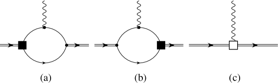
Diagrams for the $np\to d\gamma$ reaction are depicted in Fig.Β 8. The diagrams (a) and (b) in Fig.Β 8 are of LO, ${\cal O}(Q^{1/2})$, and the diagram (c) in Fig.Β 8 is of ${\cal{O}}(Q^{3/2})$, thus of a higher order. However, we will discuss below that, because of the $Vdd$ vertex involved, it would be appropriate to extract LO contribution from the (c) diagram, which is of the same order as that of the (a) and (b) diagrams.

Refer to caption
Figure 8: Diagrams contributing to $np\to d\gamma$: Diagrams (a) and (b) are of ${\cal{O}}(Q^{1/2})$, while diagram (c) is of ${\cal{O}}(Q^{3/2})$. The single lines, the double lines with a filed circle, and the wavy lines denote nucleons, dibaryons, and photons, respectively. The double line with a filed circle, which is obtained in Fig.Β 10 in Appendix, represents the propagation of ${}^{3}S_{1}$ and ${}^{1}S_{0}$ states in the intermediate state and the wave function normalization factor $\sqrt{Z_{d}}$ in the final state.

Summing up the contributions of the diagrams (a), (b) and (c) in Fig. 8, one obtains the amplitudes for the initial ${}^{3}S_{1}$ and ${}^{1}S_{0}$ states as

$\displaystyle i{\cal A}^{(a+b+c)}({}^{3}S_{1})$ $\displaystyle=$ $\displaystyle-i(\vec{\epsilon}_{(d)}^{*}\times\vec{\epsilon}_{i})\cdot(\vec{\epsilon}_{(\gamma)}^{*}\times\hat{k})\sqrt{\frac{2\pi\gamma}{1-\gamma\rho_{d}}}\frac{2}{m_{N}}\frac{1}{-\gamma-ip+\frac{1}{2}\rho_{d}(\gamma^{2}+p^{2})}$ (34)
$\displaystyle\times\left[\frac{1+\kappa_{S}}{2m_{N}}\frac{1}{2}\rho_{d}(\gamma^{2}+p^{2})+\frac{\gamma^{2}+p^{2}}{m_{N}}L_{2}\right],$
$\displaystyle i{\cal A}^{(a+b+c)}({}^{1}S_{0})$ $\displaystyle=$ $\displaystyle\vec{\epsilon}_{(d)}^{*}\cdot(\hat{k}\times\vec{\epsilon}_{(\gamma)}^{*})\sqrt{\frac{2\pi\gamma}{1-\gamma\rho_{d}}}\frac{2}{m_{N}}\frac{1}{-\frac{1}{a_{0}}-ip+\frac{1}{2}r_{0}p^{2}}$ (35)
$\displaystyle\times\left[\frac{1+\kappa_{V}}{2m_{N}}\left(\gamma-\frac{1}{a_{0}}+\frac{1}{2}r_{0}p^{2}\right)+\frac{\gamma^{2}+p^{2}}{2m_{N}}L_{1}\right].$

Here $\vec{p}$ is the relative momentum of the two-nucleon system, and $\vec{k}$ is the momentum of the out-going photon; $p=|\vec{p}|$, $k=|\vec{k}|$, and $\hat{k}=\vec{k}/k$. $\vec{\epsilon}_{(d)}^{*}$ and $\vec{\epsilon}_{(\gamma)}^{*}$ are the polarization vectors for the out-going deuteron and photon, respectively, and $\vec{\epsilon}_{i}$ is the spin $S=1$ vector for the initial ${}^{3}S_{1}$ state. $a_{0}$ and $r_{0}$ are, respectively, the scattering length and effective range of the neutron–proton ${}^{1}S_{0}$ state. The LEC $L_{2}$ has already been fixed in the previous section using the deuteron magnetic moment $\mu_{M}$. The LEC $L_{1}$ should be fixed by experiment.

It is worth noting that the LO (${\cal O}(Q^{1/2})$) amplitude for the ${}^{3}S_{1}$ state in Eq.Β (34) vanishes with the modified counting of $L_{2}$,

$\displaystyle\left.{\cal A}^{(a+b+c)}(^{3}S_{1})\right|_{L_{2}=L_{2}^{0}}=0\,,$ (36)

where the expression of $L_{2}^{0}$ is given in Eq. (19). It is well known that the leading isoscalar transition between the scattering and bound states vanishes due to the orthogonality of the wave functions. We confirm that our treatment of the LEC $L_{2}^{0}$ satisfies this condition. Higher-order terms can give non-vanishing contribution to the isoscalar amplitude, but since they are very small compared to the dominant isovector one [42], we neglect them in following calculations.

We determine the value of $L_{1}$ in Eq.Β (35) from the cross section of $np\to d\gamma$ at the thermal energy, $\sigma^{exp}=334.2\pm 0.5$ mb [43]. The total cross section in the CM frame reads

$\displaystyle\sigma=\frac{\alpha(\gamma^{2}+p^{2})}{4p}\sum_{spin}|{\cal A}|^{2},$ (37)

where $\alpha$ is the fine structure constant, and the CM energy $E$ corresponding to the thermal neutron experiment is $E=p^{2}/m_{N}=1.264\times 10^{-8}$ MeV. Using the formula for the spin summation $\sum_{spin}|i\vec{\epsilon}_{(d)}^{*}\cdot(\hat{k}\times\vec{\epsilon}_{(\gamma)}^{*})|^{2}=2$ and including only the amplitude for the ${}^{1}S_{0}$ channel, ${\cal A}(^{1}S_{0})$ in Eq.Β (35), we obtain $L_{1}=-4.427\pm 0.015$ fm.

It is to be noted that, if $L_{1}$ is set equal to zero, i.e., $L_{1}=0$, the relevant cross section would become $\sigma(L_{1}=0)=502.3$ mb, which is about 1.5 times larger than the experimental value, i.e., $\sigma(L_{1}=0)/\sigma^{exp}\simeq$ 1.50. The magnitude of the LO cross section in the KSW scheme (Eq.Β (36) in Ref.Β [41]) is smaller than $\sigma^{exp}$ by about 13 %. Furthermore, the leading one-body operators in the potential model calculations also lead to a cross section that is smaller than $\sigma^{exp}$ by about 10 %. As is well known, most of this 10 % deficiency can be accounted for by the meson exchange currents. Thus, here again we are facing the situation that, whereas the conventional treatments indicate the dominance of the LO contributions, the dEFT results exhibit uncomfortably large higher order corrections. To solve this problem, we assume that $L_{1}$ is dominated by a leading contribution denoted by $L_{1}^{0}$ which is chosen so as to reproduce the result of ERT, and that the rest, $\delta L_{1}$ contains information about the high energy physics that has been integrated out. Thus we consider the decomposition

$\displaystyle L_{1}=L_{1}^{0}+\delta L_{1},\ \ \ L_{1}^{0}=-\frac{1}{4}(1+\kappa_{V})(r_{0}+\rho_{d}),$ (38)

where numerically $L_{1}^{0}=-5.275$ fm. If we insert the expression for $L_{1}^{0}$ into $L_{1}$ in the lagrangian, the coefficient of the $Vdd$ term becomes $-\frac{1+\kappa_{V}}{2m_{N}}\frac{r_{0}+\rho_{d}}{2\sqrt{r_{0}\rho_{d}}}$, which is the coefficient of the one-body $VNN$ interaction apart from a factor $(r_{0}+\rho_{d})/(2\sqrt{r_{0}\rho_{d}})\simeq 1.024$ (which is very close to unity). Since $L^{0}_{1}$ is ${\cal O}(Q^{-1})$ due to the factor $(r_{0}+\rho_{d})$ in Eq.Β (38), the order of diagram (c) in Fig.Β 8 becomes the same as that of diagrams (a) and (b). At LO, the total cross section reads

$\displaystyle\sigma(L_{1}^{0})$ $\displaystyle=$ $\displaystyle\frac{\pi\alpha(1+\kappa_{V})^{2}\gamma^{5}a_{0}^{2}}{pm_{N}^{4}(1-\gamma\rho_{d})}\left[1-\frac{1}{\gamma a_{0}}-\frac{\gamma}{4}(r_{0}+\rho_{d})\right]^{2}\,,$ (39)

which is the same expression as that of ERT. Numerically we have $\sigma(L_{1}^{0})=304.9$ mb. This value is very close to $\sigma_{IA}=304.5$ mb obtained in the potential model with the use of the one-body operator.

Refer to caption
Figure 9: Higher order diagrams for the reaction $np\to d\gamma$ involving the $VdNN$ vertex proportional to $L_{1}^{\prime}$. The order of diagrams is of ${\cal{O}}(Q^{5/2})$. See the caption of Fig.Β 8 as well.

Now we study higher order corrections for the $np\to d\gamma$ reaction. Higher order diagrams (${\cal O}(Q^{5/2})$) with the $VdNN$ vertex proportional to $L_{1}^{\prime}$ are depicted in Fig.Β 9. One may notice that the diagrams with the $D$-wave contribution vanish for the initial $S$-wave states and the corrections from the radii are negligible because of tiny momentum transfer in the reaction. The combined contributions of diagrams (d,e,f) in Fig.Β 9 are given by

$\displaystyle i{\cal A}^{(d+e+f)}(^{1}S_{0})$ $\displaystyle=$ $\displaystyle\vec{\epsilon}_{(d)}^{*}\cdot\left(\hat{k}\times\vec{\epsilon}_{(\gamma)}^{*}\right)\sqrt{\frac{2\pi\gamma}{1-\gamma\rho_{d}}}\frac{2}{m_{N}}\frac{1}{-\frac{1}{a_{0}}-ip+\frac{1}{2}r_{0}p^{2}}$ (40)
$\displaystyle\times\frac{\gamma^{2}+p^{2}}{2m_{N}}\sqrt{\frac{m_{N}}{2\pi}}\left(\gamma+\frac{1}{a_{0}}-\frac{1}{2}r_{0}p^{2}\right)L_{1}^{\prime}\,.$

Comparing the amplitude in Eq.Β (40) with that in Eq.Β (35), one finds that the momentum dependences of the amplitudes for the LEC’s $L_{1}$ and $L_{1}^{\prime}$ are slightly different. This difference, however, does not affect the numerical results at small energies significantly. Here we compute the M1 transition contribution to the $np\to d\gamma$ cross section, using two sets of the parameters: $\delta L_{1}=0.736$ fm and $L_{1}^{\prime}=0$, and $\delta L_{1}=0$ and $L_{1}^{\prime}=4.464$ fm5/2; these LEC’s have been fixed from $\sigma^{exp}$. Predictions for the $np\to d\gamma$ cross section at energies up to 1 MeV above the thermal neutron energy are given in TableΒ 2. A fairly good agreement is seen between the results corresponding to the two different choices of the parameter set. Our dEFT results also show reasonable agreement with the recent EFT calculationsΒ [44, 45], as well as with the potential model calculation including the exchange currentΒ [46].

E(MeV) $\sigma_{M1}(\delta L_{1})$ $\sigma_{M1}(L_{1}^{\prime})$ ΟƒM​1​(E​F​T)​[45]subscriptπœŽπ‘€1𝐸𝐹𝑇[45]\sigma_{M1}(EFT)\cite[cite]{[\@@bibref{}{r-npa00}{}{}]} $\sigma_{M1}(Av18)$[46]
$1.264\times 10^{-8}$ 334.2βˆ— 334.2βˆ— 334.2βˆ— 334.2βˆ—
$5\times 10^{-4}$ 1.668 1.668 1.667 1.668
$1\times 10^{-3}$ 1.171 1.171 1.170 1.171
$5\times 10^{-3}$ 0.4953 0.4954 0.4950 0.4954
$1\times 10^{-2}$ 0.3281 0.3281 0.3279 0.3281
$5\times 10^{-2}$ 0.09814 0.09820 0.09810 0.09820
$0.100$ 0.04969 0.04976 0.04973 0.04975
$0.500$ 0.00775 0.00782 0.00787 0.00781
$1.00$ 0.0035 0.0036 0.0036 0.00355
Table 2: M1 transition contribution to the cross section for the $np\to d\gamma$ reaction. The second and third columns are our dEFT results using the two sets of LEC’s described in the text. The fourth column shows the results of the NNLO EFT calculationΒ [45], while the fifth column gives the results of an accurate potential model calculation (Av18) including the exchange currentΒ [46]. The LEC’s in both dEFT and EFT and the strength of the exchange current in the potential model calculation are fixed at the values marked by *.

5. Discussion and conclusions

In this paper we have reexamined dEFT without pions for the deuteron reactions involving the EM probe. The EM form factors of the deuteron and the total cross sections of the $np\to d\gamma$ reaction have been calculated. We have found that the LEC’s of the $Vdd$ vertices in dEFT give much larger contributions than the corresponding terms in the previous EFT approaches. Although it has not been completely explored why the LEC terms of the $Vdd$ vertex give such large contributions in dEFT, we have proposed a practical prescription to extract the LO part of the LEC’s in such manner that this LO part mimics the leading one-body $VNN$ vertices. After the LO part is disentangled, the remainder is assumed to represent the high energy physics that has been integrated out. If one is to calculate it explicitly, one should take into account relativistic corrections, meson-exchange currents, higher partial waves, etc. However, an easy way to fix the higher order part of the LEC’s is to fit it to experimental data. We were able to confirm that the higher order corrections defined in this way are indeed small, in conformity with the general tenet of EFT.

With the LEC’s thus determined, we have calculated the form factors $A(q)$ and $B(q)$ for elastic $e$-$d$ scattering and found that the results of $A(q)$ are very close to the experimental data for momenta up to 200 MeV. Furthermore, our results of $A(q)$ and $B(q)$ are comparable to those of the accurate potential model calculation. Our estimations of the total cross sections of the $np\to d\gamma$ reaction for energies up to 1 MeV also agree well with the results of the other EFT calculations and the accurate potential model. With the proper treatment of the LEC’s in the $Vdd$ vertices, the convergence of dEFT becomes similarly efficient as other EFT’s and this can be interpreted as an indication that dEFT is a useful tool for understanding a wide class of low-energy phenomena involving the deuteron and an external probe.

Acknowledgments

We thank S. Nakamura for providing us his numerical results in Table 1 and communications. We also thank K. Kubodera for reading the manuscript. S.A. thanks U. van Kolck, M. Oka, R.Β H. Cyburt, W. Detmold, J.-W. Chen, A. Parreno, P.Β F. Bedaque, S.Β R. Beane, T. Sato, F. Myhrer, H.Β W. Fearing, and M.Β J. Savage for discussions and communications. This work is supported in part by the Natural Sciences and Engineering Research Council of Canada and by the Korea Research Foundation (Grant No. KRF-2003-070-C00015).

Appendix

In this appendix we rederive the two-nucleon(dibaryon) propagators and fix the LEC’s using the known properties of $NN$ systems in the $S$-wave channels; see also Ref.Β [19].

LO diagrams for the two-nucleon(dibaryon) propagators in the $S$-wave channels are depicted in Fig.Β 10. Since the insertion of the two-nucleon one-loop diagram does not alter the order of the diagramΒ [8, 12, 13, 18], the two-nucleon bubbles in the propagators should be summed up to infinite order.

Refer to caption
Figure 10: Diagrams for the two-nucleon(dibaryon) propagator at leading order: a double (single) line stands for the dibaryon (nucleon) field.

Thus the inverse two-nucleon(dibaryon) propagators in the center-of-mass (CM) frame read

$\displaystyle iD_{t,s}^{-1}(p)$ $\displaystyle=$ i​σt,s​(E+Ξ”t,s)+i​yt,s2​mN4​π​(ΞΌ+i​p)𝑖subscriptπœŽπ‘‘π‘ πΈsubscriptΔ𝑑𝑠𝑖superscriptsubscript𝑦𝑑𝑠2subscriptπ‘šπ‘4πœ‹πœ‡π‘–π‘\displaystyle i\sigma_{t,s}(E+\Delta_{t,s})+iy_{t,s}^{2}\frac{m_{N}}{4\pi}(\mu+ip) (41)
$\displaystyle=$ i​mN​yt,s24​π​[4​π​σt,s​Δt,smN​yt,s2+ΞΌ+4​π​σt,s​EmN​yt,s2+i​p],𝑖subscriptπ‘šπ‘superscriptsubscript𝑦𝑑𝑠24πœ‹delimited-[]4πœ‹subscriptπœŽπ‘‘π‘ subscriptΔ𝑑𝑠subscriptπ‘šπ‘superscriptsubscript𝑦𝑑𝑠2πœ‡4πœ‹subscriptπœŽπ‘‘π‘ πΈsubscriptπ‘šπ‘superscriptsubscript𝑦𝑑𝑠2𝑖𝑝\displaystyle i\frac{m_{N}y_{t,s}^{2}}{4\pi}\left[\frac{4\pi\sigma_{t,s}\Delta_{t,s}}{m_{N}y_{t,s}^{2}}+\mu+\frac{4\pi\sigma_{t,s}E}{m_{N}y_{t,s}^{2}}+ip\right],

where $\mu$ is the renormalization scale of the PDS scheme, $p$ is the magnitude of the nucleon momentum in the CM frame, and $E$ is the total energy $E\simeq p^{2}/m_{N}$.

The two-nucleon(dibaryon) propagator in the spin singlet state, $D_{s}(p)$, can be renormalized using the ${}^{1}S_{0}$ channel $NN$ scattering amplitude.131313 Although it is known that the expansion series of the ERT parameters in the ${}^{1}S_{0}$ channel converges well, we employ the modified counting rule $Q\sim\{p,a_{0}^{-1},r_{0}^{-1}\}$ for the ${}^{1}S_{0}$ channel as well.

Refer to caption
Figure 11: Diagrams for the $NN$ scattering amplitudes. Diagram (a) is for $S$- to $S$-wave channel and diagram (b) is for $D$- to $S$-wave channel. The $dNN$ vertex with (without) a filled box denotes a vertex proportional to $C_{2}^{(sd)}$ ($y_{t,s}$). The propagator of the two-nucleon(dibaryon) filed (a double line with a filled circle) is obtained from the diagrams in Fig.Β 10.

The amplitude obtained from Fig.Β 11 (a) reads

iβ€‹π’œs𝑖subscriptπ’œπ‘ \displaystyle i{\cal A}_{s} $\displaystyle=$ (βˆ’i​ys)​(i​Ds​(p))​(βˆ’i​ys)=4​πmN​1βˆ’4​π​σs​ΔsmN​ys2βˆ’ΞΌβˆ’4​π​σsmN2​ys2​p2βˆ’i​p,𝑖subscript𝑦𝑠𝑖subscript𝐷𝑠𝑝𝑖subscript𝑦𝑠4πœ‹subscriptπ‘šπ‘14πœ‹subscriptπœŽπ‘ subscriptΔ𝑠subscriptπ‘šπ‘superscriptsubscript𝑦𝑠2πœ‡4πœ‹subscriptπœŽπ‘ superscriptsubscriptπ‘šπ‘2superscriptsubscript𝑦𝑠2superscript𝑝2𝑖𝑝\displaystyle(-iy_{s})(iD_{s}(p))(-iy_{s})=\frac{4\pi}{m_{N}}\frac{1}{-\frac{4\pi\sigma_{s}\Delta_{s}}{m_{N}y_{s}^{2}}-\mu-\frac{4\pi\sigma_{s}}{m_{N}^{2}y_{s}^{2}}p^{2}-ip}, (42)

and it is related to the $S$-matrix via

Sβˆ’1=e2​i​δ0βˆ’1=2​i​pp​cot​δ0βˆ’i​p=i​(p​mN2​π)β€‹π’œs,𝑆1superscript𝑒2𝑖subscript𝛿012𝑖𝑝𝑝cotsubscript𝛿0𝑖𝑝𝑖𝑝subscriptπ‘šπ‘2πœ‹subscriptπ’œπ‘ \displaystyle S-1=e^{2i\delta_{0}}-1=\frac{2ip}{p\,{\rm cot}\delta_{0}-ip}=i\left(\frac{pm_{N}}{2\pi}\right){\cal A}_{s}, (43)

where $\delta_{0}$ is the phase shift for the ${}^{1}S_{0}$ channel. Meanwhile effective range expansion (ERE) reads

$\displaystyle p\,{\rm cot}\delta_{0}$ $\displaystyle=$ $\displaystyle-\frac{1}{a_{0}}+\frac{1}{2}r_{0}p^{2}+\cdots,$ (44)

where $a_{0}$ (= $-$23.71 fm) is the scattering length and $r_{0}$ (= 2.73 fm) the effective range in the ${}^{1}S_{0}$ channel. Inserting Eq.Β (44) into Eq.Β (43), one obtains Οƒs=βˆ’1subscriptπœŽπ‘ 1\sigma_{s}=-1, and

$\displaystyle y_{s}=\frac{2}{m_{N}}\sqrt{\frac{2\pi}{r_{0}}},\ \ \ D_{s}(p)=\frac{m_{N}r_{0}}{2}\frac{1}{\frac{1}{a_{0}}+ip-\frac{1}{2}r_{0}p^{2}}\,.$ (45)

Now we fix the LEC’s in the coupled channel. Diagrams for the ${}^{3}S_{1}-{}^{3}D_{1}$ channel are depicted in Figs.Β 11 (a, b). Each of the amplitudes reads

$\displaystyle{\cal A}_{[SS]}$ $\displaystyle=$ $\displaystyle\frac{4\pi}{m_{N}}\frac{1}{-\frac{4\pi\sigma_{t}\Delta_{t}}{m_{N}y_{t}^{2}}-\mu-\frac{4\pi\sigma_{t}}{m_{N}^{2}y_{t}^{2}}p^{2}-ip}\,,$ (46)
$\displaystyle{\cal A}_{[DS]}$ $\displaystyle=$ $\displaystyle\frac{\sqrt{2}}{3}\frac{C_{2}^{(sd)}p^{2}}{y_{t}\sqrt{m_{N}\rho_{d}}}\frac{4\pi}{m_{N}}\frac{1}{-\frac{4\pi\sigma_{t}\Delta_{t}}{m_{N}y_{t}^{2}}-\mu-\frac{4\pi\sigma_{t}}{m_{N}^{2}y_{t}^{2}}p^{2}-ip}\,.$ (47)

The relation between the $S$-matrix and the amplitudes in the coupled channel is given by

$\displaystyle S$ $\displaystyle=$ $\displaystyle 1+i\frac{pm_{N}}{2\pi}\left(\matrix{{\cal A}_{[SS]}&{\cal A}_{[DS]}\cr{\cal A}_{[SD]}&{\cal A}_{[DD]}}\right)=\left(\matrix{e^{2i\bar{\delta}_{0}}{\rm cos}2\bar{\epsilon}_{1}&ie^{i(\bar{\delta}_{0}+\bar{\delta}_{2})}{\rm sin}2\bar{\epsilon}_{1}\cr ie^{i(\bar{\delta}_{0}+\bar{\delta}_{2})}{\rm sin}2\bar{\epsilon}_{1}&e^{2i\bar{\delta}_{2}}{\rm cos}2\bar{\epsilon}_{1}}\right),$ (48)

where we have employed a convention for the phase shifts defined in Ref.Β [47].

Since it is known that $\bar{\epsilon}_{1}$ is numerically small, we put $\cos(2\bar{\epsilon_{1}})\simeq 1$. Around the deuteron pole, ERE readsΒ [23],

$\displaystyle p\,{\rm cot}\bar{\delta}_{0}=-\gamma+\frac{1}{2}\rho_{d}(p^{2}+\gamma^{2})+\cdots,$ (49)

with $\gamma^{-1}=4.319$ fm and $\rho_{d}=1.764$ fm. Following the same steps that lead to Eq.Β (45), one obtains $\sigma_{t}=-1$, and

$\displaystyle y_{t}=\frac{2}{m_{N}}\sqrt{\frac{2\pi}{\rho_{d}}},\ \ \ D_{t}(p)=\frac{m_{N}\rho_{d}}{2}\frac{1}{\gamma+ip-\rho_{d}\frac{1}{2}(\gamma^{2}+p^{2})}=\frac{Z_{d}}{E+B}+\cdots,$ (50)

where $Z_{d}$ is the wave function normalization factor of the deuteron around the pole of the deuteron binding energy $B$, and the ellipsis in Eq. (50) denotes corrections that are finite or vanish at $E=-B$. Thus one obtainsΒ [19]

$\displaystyle Z_{d}=\frac{\rho_{d}\gamma}{1-\rho_{d}\gamma}\,.$ (51)

Next we renormalize the coupled channel amplitude ${\cal A}_{[DS]}$ at the deuteron pole $p=i\gamma$ through the relation,

βˆ’2​(Ξ·s​d1βˆ’Ξ·s​d2)=tan​(2​ϡ¯1)sin​(δ¯0βˆ’Ξ΄Β―2)|p=i​γ=2β€‹π’œ[S​D]π’œ[S​S]βˆ’π’œ[D​D]|p=iβ€‹Ξ³β‰ƒβˆ’13​mNπ​C2(s​d)​γ2,2subscriptπœ‚π‘ π‘‘1superscriptsubscriptπœ‚π‘ π‘‘2evaluated-attan2subscriptΒ―italic-Ο΅1sinsubscript¯𝛿0subscript¯𝛿2𝑝𝑖𝛾evaluated-at2subscriptπ’œdelimited-[]𝑆𝐷subscriptπ’œdelimited-[]𝑆𝑆subscriptπ’œdelimited-[]𝐷𝐷𝑝𝑖𝛾similar-to-or-equals13subscriptπ‘šπ‘πœ‹superscriptsubscript𝐢2𝑠𝑑superscript𝛾2\displaystyle-2\left(\frac{\eta_{sd}}{1-\eta_{sd}^{2}}\right)=\left.\frac{{\rm tan}(2\bar{\epsilon}_{1})}{{\rm sin}(\bar{\delta}_{0}-\bar{\delta}_{2})}\right|_{p=i\gamma}=\left.\frac{2{\cal A}_{[SD]}}{{\cal A}_{[SS]}-{\cal A}_{[DD]}}\right|_{p=i\gamma}\simeq-\frac{1}{3}\sqrt{\frac{m_{N}}{\pi}}C_{2}^{(sd)}\gamma^{2}, (52)

where we have neglected the $D$-wave amplitude ${\cal A}_{[DD]}$. Thus, neglecting the Ξ·s​d2superscriptsubscriptπœ‚π‘ π‘‘2\eta_{sd}^{2} correction in the relation above, one obtains

$\displaystyle C_{2}^{(sd)}$ $\displaystyle\simeq$ 6​πmN​ηs​dΞ³2.6πœ‹subscriptπ‘šπ‘subscriptπœ‚π‘ π‘‘superscript𝛾2\displaystyle 6\sqrt{\frac{\pi}{m_{N}}}\frac{\eta_{sd}}{\gamma^{2}}\,. (53)

References

  • [1] S. Weinberg, hep-th/9702027.
  • [2] S.Β R. Beane, P.Β F. Bedaque, M.Β J. Savage, and U. van Kolck, Nucl. Phys. A 700 (2002) 377.
  • [3] S. Weinberg, Phys. Lett. B 251 (1990) 288.
  • [4] C. OrdonαΊ½z, L. Ray and U. van Kolck, Phys. Rev. C 53 (1996) 2086.
  • [5] T.-S. Park, K. Kubodera, D.-P. Min and M. Rho, Nucl. Phys. A 646 (1999) 83.
  • [6] C.Β H. Hyun, T.-S. Park and D.-P. Min, Phys. Lett. B 473 (2000) 6.
  • [7] E. Epelbaum, W. Gloeckle and U.-G. Meißner, Nucl. Phys. A 671 (2000) 295.
  • [8] D.Β B. Kaplan, M.Β J. Savage and M.Β B. Wise, Phys. Lett. B 424 (1998) 390.
  • [9] S. Fleming, T. Mehen, and I.Β W. Stewart, Nucl. Phys. A 677 (2000) 313.
  • [10] S.Β R. Beane el al., in (ed.) M. Shifman, At the frontier of particle physics, Vol.1 133, World Scientific, Singapore (2001); nucl-th/0008064.
  • [11] P.Β F. Bedaque and U.Β van Kolck, Ann. Rev. Nucl. Part. Sci. 52 (2002) 339.
  • [12] U. van Kolck, Nucl. Phys. A 645 (1999) 273.
  • [13] J. Gegelia, Contribution to Workshop on Methods of Nonperturbative Quantum Field Theory, Adelaide, Australia, 2-13 Feb. 1998: nucl-th/9802038.
  • [14] M. Rho, AIP Conf. Proc. 494 (1999) 391; nucl-th/9908015.
  • [15] D.Β R. Phillips and T.Β D. Cohen, Nucl. Phys. A 668 (2000) 45.
  • [16] D.Β R. Phillips, G. Rupak, and M.Β J. Savage, Phys. Lett. B 473 (2000) 209.
  • [17] D.Β B. Kaplan, Nucl. Phys. B 494 (1997) 471.
  • [18] P.Β F. Bedaque and U. van Kolck, Phys. Lett. B 428 (1998) 221.
  • [19] S.Β R. Beane and M.Β J. Savage, Nucl. Phys. A 694 (2001) 511.
  • [20] J.Β F. Beacom and S.Β J. Parke, Phys. Rev. D 64 (2001) 091302.
  • [21] S. Ando, H.Β W. Fearing, V. Gudkov, K. Kubodera, F. Myhrer, T. Sato, and S. Nakamura, Phys. Lett. B 595 (2004) 250, nucl-th/0402100.
  • [22] W. Detmold and M.Β J. Savage, Nucl. Phys. A 743 (2004) 170.
  • [23] H.Β A. Bethe, Phys. Rev. 76 (1949) 38.
  • [24] R.Β B. Wiringa, V.Β G.Β J. Stoks, and R. Schiavilla, Phys. Rev. C 51 (1995) 38.
  • [25] N. Fettes, U.-G. Meißner, M. MojΕΎiΕ‘, and S. Steininger, Annals. Phys. 283 (2000) 273; Erratum ibid. 288 (2001) 249.
  • [26] D.Β R. Phillips, Phys. Lett. B 567 (2003) 12.
  • [27] D.Β B. Kaplan, M.Β J. Savage, and M.Β B. Wise, Phys. Rev. C 59 (1999) 617.
  • [28] J.-W. Chen, G. Rupak, and M.Β J. Savage, Nucl. Phys. A 653 (1999) 386.
  • [29] P. J. Mohr and B. N. Taylor, Rev. Mod. Phys. 72 (2000) 351.
  • [30] T. E. O. Ericson and M. Rosa-Clot, Nucl. Phys. A 405 (1983) 497.
  • [31] I. Sick and D. Trautmann, Nucl. Phys. A 635 (1998) 559.
  • [32] T.-S. Park, K. Kubodera, D.-P. Min, and M. Rho, Phys. Rev. C 58 (1998) R637.
  • [33] J.-W. Chen, X. Ji, and Y. Li, Phys. Lett. B 603 (2004) 6.
  • [34] V. Bernard, H.Β W. Fearing, T.Β R. Hemmert, and U.-G. Meißner, Nucl. Phys. A 635 (1998) 121; Erratum ibid. A 642 (1998) 563.
  • [35] J.-W. Chen, G. Rupak, and M.Β J. Savage, Phys. Lett. B 464 (1999) 1.
  • [36] P. Mergell et al., Nucl. Phys. A 596 (1996) 367.
  • [37] V.Β Z. Jankus, Phys. Rev. 102 (1956) 1586.
  • [38] G.Β G. Simon, Ch. Schmitt, and V.Β H. Walther, Nucl. Phys. A 364 (1981) 285.
  • [39] M. Garcon and J.Β W. Van Orden, Adv. Nucl. Phys. 26 (2001) 293.
  • [40] T.-S. Park, D.-P. Min and M. Rho, Phys. Rev. Lett. 74 (1995) 4153
  • [41] M.Β J. Savage, K.Β A. Scaldeferri, and M.Β B. Wise, Nucl. Phys. A 652 (1999) 273.
  • [42] T.-S. Park, K. Kubodera, D.-P. Min and M. Rho, Phys. Lett. B 472 (2000) 232.
  • [43] A.Β E. Cox, S.Β A.Β R. Wynchank and C.Β H. Colli, Nucl. Phys. 74 (1965) 497.
  • [44] J.-W. Chen and M.Β J. Savage, Phys. Rev. C 60 (1999) 065205.
  • [45] G. Rupak, Nucl. Phys. A 678 (2000) 405.
  • [46] S. Nakamura, T. Sato, V. Gudkov, K. Kubodera, Phys. Rev. C 63 (2001) 034617.
  • [47] H.Β P. Stapp, T.Β J. Ypsilantis, and N. Metropolis, Phys. Rev. 105 (1957) 302.