The meaning of S-D dominance

Abstract

The dominance of S and D pairs in the description of deformed nuclei is one of the facts that provided sustain to the Interacting Boson Approximation. In Ref.[1], using an exactly solvable model with a repulsive pairing interaction between bosons it has been shown that the ground state is described almost completely in terms of S and D bosons. In the present paper we study the excited states obtained within this exactly solvable hamiltonian and show that in order to obtain a rotational spectra all the other degrees of freedom are needed.

I Introduction

The interacting boson approximation (IBA)[2, 3, 4] assumes that the elementary excitation used for the description of the low energy nuclear spectra in open shell nuclei are formed by pairs of nucleons coupled to angular momentum 0 and 2 (S and D). These excitations behave in this approximation as bosons. An intriguing question is how to determine the structure of these S and D bosons:

It seems natural to use the Hartree-Fock-Bogoliubov (HFB) approximation where the ground state wave function can be written as in Ref. [5].

$$|\Phi>=Nexp(\frac{1}{2}\sum_{kl}Z_{kl}a_{k}^{\dagger}a_{l}^{\dagger}),$$ (1)

where $a_{k}^{\dagger}$ creates a particle in a state $k$, $N$ is a normalization constant and $Z$ is the antisymmetric structure matrix[6, 7].

In order to study this point it may be enough to use the results obtained with schematic calculations using the pairing plus quadrupole hamiltonian in the Nilsson+BCS approximation. These calculations show that the S and D bosons are dominant in the description of the ground state if it is considered a coherent state of Cooper pairs[8]or as a pair condensate[9]. However, self consistent HFB calculations for the single j-shell[10] or many shells[11, 12] using unrenormalized simple interactions show that, in these cases, the space spanned by the S and D pairs does not provide a reasonable description of well-deformed systems. In Ref. [13] it is shown that if the interaction strengths are renormalized to reproduce the value of $\beta$ (deformation parameter) and $\Delta$ (the superconductive gap) a reasonable description of the ground state of well-deformed nuclei is obtained.

In Ref.[14] a large group of integrable many body hamiltonians (as well as the constants of motion related to them) was found. One of these hamiltonians is a repulsive pairing interaction between bosons with single boson energies that may have any value. For a particular set of single particle energies and a repulsive pairing interaction they found that for a large number of bosons ($N$) the ground state of the system only contains two types of bosons (in that paper the relevant bosons were S and P, all other bosons have occupations numbers of order $\frac{1}{N}$). The reason why it is interesting to consider this hamiltonian is that the repulsive pairing interaction between the bosons mucks up the influence of the Pauli principle between the quasibosons built on fermion pair (see Appendix 1 for a description of this relation in the single j-shell case). In a recent letter[1] a renormalized pairing interaction as well as a set of single boson s energies more related to the nuclear case yields that the S and D states are the only ones that have large occupations numbers. In Ref.[15] a similar calculation is done using group theoretical methods (therefore they are forced to use the pairing interaction instead of the renormalized one) and the S-D dominance is attributed to the choice of boson’s energies.
The present paper uses the recently proposed Richardson-Gaudin (RG) integrable models [14] (for a recent review see [16]) to study the excitations obtained when using a repulsive pairing interaction between bosons for “realistic” situations. By “realistic” situations we mean the use of single boson’s energies similar to the ones that correlated pairs of nucleons have in nuclei. The strength of the pairing interaction is used as a free parameter. It must be noted that for the single j-shell the value of the pairing interaction between the “bosons” is minus the pairing interaction between fermions, as shown in Appendix 1. The use of this treatment allows for the study of two problems: the first one is the influence of using realistic values for the boson energies on the S-D dominance as well as for the interaction strength; the second one is the possibility of constructing a rotational spectra if a multiboson space is considered.

II Hamiltonian used and its treatment

The hamiltonian that will be used is

$$H=\sum_{l}\epsilon_{l}\hat{n}_{l}+\frac{g}{2}\sum_{kl}(K_{k}^{+}K_{l}^{-}+K_{k}^{-}K_{l}^{+}),$$ (2)

where $\epsilon_{l}$ is the energy of the boson $l$ and the operators $K_{i}^{+}=$ and $K_{i}^{-}$ are the generators of an SU(1,1) algebra. The set of generators $K_{i}^{0}=\frac{1}{2}\hat{n}_{l}+\frac{\Omega_{i}}{4}$, $K_{i}^{+}$ and $K_{i}^{-}=(K_{i}^{+})^{{\dagger}}$ satisfies the commutation relations

$$\left[K_{i}^{0},K_{j}^{+}\right] = +\delta_{ij}K_{i}^{+}~{},~{}\left[K_{i}^{0},K_{j}^{-}\right]=-\delta_{ij}K_{i}^{-}~{},$$ (3)

$$\left[K_{i}^{+},K_{j}^{-}\right]=-2\delta_{ij}K_{i}^{0}.$$

This SU(1,1) algebra is realized in terms of operators that create and annihilate bosons. In the usual pseudo-spin representation, the generators can be written as

$$K_{j}^{0}=\frac{1}{2}\sum_{m}a_{jm}^{\dagger}a_{jm}+\frac{\Omega_{j}}{4}\text{ \ ,}~{}~{}K_{j}^{+}=\frac{1}{2}\sum_{m}a_{jm}^{\dagger}a_{j\bar{m}}^{\dagger}\text{ \ },$$ (4)

where $a_{jm}^{\dagger}\left(a_{jm}\right)$ creates (annihilates) a boson in the state $|jm\rangle$, $|j\bar{m}\rangle$ is the state obtained by acting with the time reversal operator on the state $|jm\rangle$, and $\Omega_{j}$ is the total degeneracy of the single-boson level $j$. Here the realization involves correlated pair operators. It is simple to express the pairing hamiltonian in terms of these operators.

The Hilbert space of $N$ particles moving in shells $k,l,m,....p$ can be classified in terms of the product of groups SU(1,1)${}_{k}\times$SU(1,1) ${}_{l}\times$SU(1,1)${}_{m}\times......$SU(1,1)_p. All the states of the Hilbert space can be written as

$$|n_{k},...,n_{p,}\nu>=\frac{1}{\sqrt{{\cal N}}}(K_{k}^{+})^{n_{k}}....(K_{p}^{+})^{n_{p}}|\nu>,$$ (5)

where  ${\cal N}$ is a normalization constant. The possible numbers of pairs in each level is $0\leq n_{s}<N$ and the states $|\nu>=|\nu_{k},\nu_{l},\nu_{m},...\nu_{p}>$ of unpaired particles are defined as

$$K_{s}^{-}|\nu>=0,\text{ \ \ \ \ }\hat{n}_{s}|\nu>=\nu_{s}|\nu>,\text{ \ \ \ \ \ }K_{s}^{0}|\nu>=d_{s}|\nu>$$ (6)

where $d_{s}=\frac{1}{4}(2\nu_{s}+\Omega_{s})$ and $N=2M+\nu,$ N being the total number of bosons, M the total number of pairs and  $\nu$ (usually called the total seniority) the total number of unpaired bosons that is the sum of all the $\nu_{s}$.

There are three families of fully integrable and exactly-solvable RG models that derive from these SU(1,1) algebras, which are referred to as the rational, trigonometric and hyperbolic models, respectively [14]. The pairing interaction is related to the “rational” family, for which they express the integrals of motion in terms of the above generators as

$$R_{i}=K_{i}^{0} + 2g\sum_{i(\neq j)}\left\{\frac{1}{2(\epsilon_{i}-\epsilon_{j})}[K_{i}^{+}K_{j}^{-}+K_{i}^{-}K_{j}^{+}]\right.$$ (7)

$$~{}~{}~{}~{}~{}\left.-~{}\frac{1}{(\epsilon_{i}-\epsilon_{j})}K_{i}^{0}K_{j}^{0}\right\}.$$

For each degree of freedom $i$, there is one real arbitrary parameter that in the rational model is equal to $\epsilon_{i}$ that enters the integrals of motion. It can be easily checked that these operators commute among themselves, and each one commutes with the operator $K^{0}=\sum_{i}K^{0}_{i}$.

The eigenvalue equation $R_{i}|\Psi_{i}\rangle=r_{i}|\Psi_{i}\rangle$ can be readily solved using methods analogous to those first introduced by Richardson to treat the quantum pairing problem [17]. The eigenvectors take the form

$$\left|\Psi\right\rangle=\prod_{\alpha=1}^{M}B_{\alpha}^{\dagger}\left|\nu\right\rangle,\quad B_{\alpha}^{\dagger}=\sum_{l}\frac{1}{(e_{\alpha}-\epsilon_{l})}~{}K_{l}^{+},$$ (8)

where $|\nu\rangle$ is a state that is annihilated by all the $K_{i}^{-}$ and $M$ is equal to the number of collective $B^{+}$ operators that comprise the state. The structures of the collective operators are determined by a set of $M$ parameters $e_{\alpha}$, which satisfy the set of coupled nonlinear equations

$$1+4g\sum_{j}\frac{d_{j}}{2\epsilon_{j}-e_{\alpha}}+4g\sum_{\beta\left(\neq\alpha\right)}\frac{1}{e_{\beta}-e_{\alpha}}=0.$$ (9)

The associated eigenvalues take the form

$$r_{i}=d_{i}\left\{1-2g\sum_{j\left(\neq i\right)}\frac{d_{j}}{\epsilon_{i}-\epsilon_{j}}+4g\sum_{\alpha}\frac{1}{e_{\alpha}-2\epsilon_{i}}\right\}.$$ (10)

We note here that each independent solution of the set on nonlinear coupled equations (9) defines an eigenstate (8) and eigenvalues that are given by

$$E=2g\sum_{\alpha}e_{\alpha}.$$ (11)

Following Richardson [17], the occupation numbers can be calculated as

$$\left\langle n_{\lambda}\right\rangle=\left\langle\frac{\partial H_{P}}{\partial\epsilon_{l}}\right\rangle=\sum_{\alpha}\frac{\partial e_{\alpha}}{\partial\epsilon_{l}}~{}.$$ (12)

From (2), and making use of (9) and (11), a set of $M$ coupled linear equations in terms of $M$ new unknowns can be obtained, which give the $\lambda$ boson occupation numbers. Details of the derivation can be found in ref. [19]. Dividing these occupation numbers by the total number of bosons we obtain the occupation probabilities of the different bosons.

III Results and discussion

In order to relate the calculation to the nuclear case it is necessary to choose the properties of the boson degrees of freedom for each angular momentum as well as the coupling constant. The microscopic image that we have in mind is the Nilsson model and therefore it seems natural to consider only one type of bosons for each even angular momentum. For angular momentum two the seniorities needed to describe the low lying states are well known [18] from the study of the five dimensional harmonic oscillator. For $\lambda=2$ we will consider only states with seniority one (J=2), two (J=2 and 4) and three (J=0,3,4,6)). A similar treatment can be used for the $\lambda$ bosons (the first excited states corresponding to these degrees of freedom will have seniority one and angular momentum $J=\lambda$ and are the only ones that we will consider). It is worthwhile to remark that as the Hamiltonian has vanishing matrix elements between states with different seniorities, the states connected by the hamiltonian must have the same seniorities. There are too many parameters if the boson’s single particle energies are left as free parameters. We performed all our calculation with a large but meaningful number of bosons (40) and we choose the single boson energies by imposing the condition that the ratios of calculated energies of the first $2^{+}$, $4^{+}$, $6^{+}$ and $8^{+}$ states are as close as possible to the values provided by the rigid rotor for $G/h\nu_{2}=.72$ (for this value of $G/h\nu_{2}$ the ratios of the energies of the ground state band have reached what we can consider their asymptotic values) taking into account bosons with all the even angular momentum up to 12. As we do not know the ground state energy, we can only determine the differences between the bosons single particle energies. We define our energy scale by making the difference of energy between the $\lambda=2$ and $\lambda=0$ bosons equal to one. The resulting energy differences (to the J=0 boson) have values which are reasonables: E${}_{4}=1.25$; E${}_{6}=1.50$; E${}_{8}=2.12$; E${}_{10}=2.28$ and ; E${}_{12}=2.42$.

In Fig. 1 we show the excitation energy of the $2_{1}$ state as function of $G/h\nu_{2}$ (being $h\nu_{2}$ the energy of the $\lambda=2$ boson). The asymptotic value ($\approx.124$) provides us with an absolute energy scale. If this state is the $2_{1}$ state of the ground state rotational band the energies are of the right order of magnitude and $G/h\nu_{2}$ must have a value of the order of 0.2 to reproduce the fermionic strength.

Figure 1: Energy of the $2_{1}$ state as function of the scaled strength parameter $G/h\nu_{2}$.

Initially we include all bosons with even angular momentums up to $\lambda=12$. In Fig. 2 we show the ratio between the energy of the first state for each even angular momentum (up to J=12) to the $2_{1}$ state as function of $G/h\nu_{2}$. It is evident the departure from the rigid rotor values when the angular momentum increases or $G$ decreases. In the region of $G/h\nu_{2}\approx 0.2$ the structure of the excitations is similar to the rigid rotor. For the model we are using, the states are labeled by the seniority of the different bosons. To get a feeling of the types of result obtained in table 1 we list the excitation energies for $G/h\nu_{2}=0.72$ for some selected sates, showing also the possible angular momentum of these states. It follows that there are many excited levels in the low energy region and that it is difficult to recognize the excited rotational bands.

Table 1: Excitation energies, in units of $h\nu_{2}$, for the three first solutions with the seniorities displayed in the table. A list of all the angular momentum related with this seniority structure are given in the last column.

$\tilde{M}$	$\nu_{J=0}$	$\nu_{J=2}$	$\nu_{J=4}$	$\nu_{J=6}$	$\nu_{J=8}$	$E_{1}$	$E_{2}$	$E_{3}$	$Possible~{}angular~{}momentums$
20	0	0	0	0	0	0.00000	0.59667	1.35124	$0$
19	1	1	0	0	0	0.12424	0.79629	1.51183	$2$
19	1	0	1	0	0	0.41361	0.99778	1.79228	$4$
19	1	0	0	1	0	0.86824	1.46588	2.18733	$6$
19	1	0	0	0	1	1.54591	2.14410	2.88702	$8$
19	0	2	0	0	0	0.29651	1.03966	1.72393	$2,4$
18	1	3	0	0	0	0.51105	1.32094	1.98002	$0,3,4,6$
18	1	2	1	0	0	0.75453	1.50430	2.21865	$0,1,2^{2},3^{2},4^{2},5^{2},6^{2},7,8$
18	1	2	0	1	0	1.19265	1.95006	2.59798	$2,3,4^{2},5^{2},6^{2},7^{2},8^{2},9,10$
18	0	3	1	0	0	0.993228	1.81334	2.50029	$0,1^{2},2^{3},3^{3},4^{4},5^{3},6^{3},7^{3},8^{2},9,10$

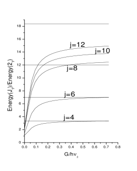
Figure 2: Ratio of the energy of the $J_{1}$ states to the energy of the $2_{1}$ state as function of the scaled strength parameter $G/h\nu 2$ for a calculation that includes all even values of J up to 12. The rigid rotor values are shown to guide the eye.

In Fig. 3 we show the occupation probabilities of the different boson levels obtained for some selected states. In general only two boson levels are populated (the S and D bosons share more than 85% of the occupation probabilities). The contribution of the $\lambda=0$ boson will be more important if we increase the number of bosons or if we consider a renormalized interaction as the one used in Ref.[1].

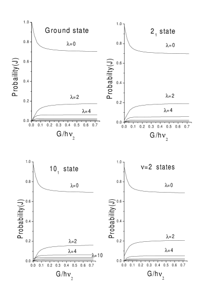
Figure 3: Occupation probabilities of the different $\lambda$ bosons as function of the scaled strength parameter $G/h\nu_{2}$ for a calculation that includes all even values of $\lambda$ up to 12. The lines corresponding to sizeable contributions are labelled by $\lambda$.

In Table 2 we show the occupation probabilities for the different boson degrees of freedom for $G/h\nu_{2}=0.72$ and for the first state corresponding to different seniorities. From this table follows that the contributions of the different bosons (with seniority one)are important in the description of the ground state band, even if the occupation probabilities are small.

Table 2: Occupation probabilities for the bosons with angular momentum J of the first states of a given seniority for the calculation that includes all even J up to 12 with $G=0.72$. In the last column are indicated the structure and angular momentums of the corresponding states

P(J=0)	P(J=2)	P(J=4)	P(J=6)	P(J=8)	P(J=10)	P(J=12)	$States$
0.70384	0.17515	0.06277	0.02505	0.01092	0.01104	0.01124	J=0 ($\nu_{i}=0$)
0.69740	0.19038	0.05658	0.02372	0.01048	0.01062	0.01082	J=2 ($\nu_{2}$=1)
0.69807	0.14543	0.09903	0.02464	0.01079	0.01092	0.01112	J=4 ($\nu_{4}$=1)
0.69602	0.15579	0.06154	0.05365	0.01085	0.01098	0.01118	J=6 ($\nu_{6}$=1)
0.69431	0.15963	0.06183	0.02489	0.03715	0.01099	0.01120	J=8 ($\nu_{8}$=1)
0.69405	0.16008	0.06186	0.02489	0.01087	0.03704	0.01120	J=10($\nu_{10}=1)$
0.69386	0.16040	0.06189	0.02490	0.01087	0.01100	0.03710	J=12($\nu_{12}=1)$
0.68952	0.20713	0.05060	0.02228	0.00999	0.01014	0.01034	J=2,4 ($\nu_{2}$=2)
0.68055	0.22453	0.04514	0.02082	0.00964	0.00964	0.00984	J=0,3,4,6 ($\nu_{2}=3)$

A question that one may ask is how will change the description obtained as we diminished the number of boson degrees of freedoms. For that purpose we also performed the calculation including only bosons up to $\lambda=8$. We tried again to reproduce as well as possible the rigid rotor by changing the bosons energies. The values obtained for the energies (in the region of large G) were E${}_{4}=1.10$; E${}_{6}=1.37$; E${}_{8}=2.11$ which are similar to the values used in the larger calculation. The asymptotic value for the $2^{+}$ energy was $0.101$.

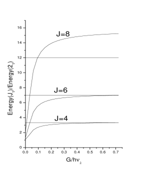
Figure 4: Ratio of the energies of the $J_{1}$ states to the energy of the $2_{1}$ state as function of the scaled strength parameter $G/h\nu 2$ for a calculation that includes all even values of $\lambda$ up to 8. The rigid rotor values are shown to guide the eye.

In Fig. 4 we show results similar to Fig. 2 but using the smaller space. It is clear that we are not able to reproduce properly the $8^{+}$ state which gives an indication of the importance of the $\lambda=10$ and $\lambda=12$ bosons in its description. In Figure 5 we display the occupation probabilities for this case and in Table 3 we reproduce the equivalent of Table 2.

Table 3: Occupation probabilities for the bosons with angular momentum J of the first states of a given seniority for the calculation that includes all even J up to 8 with $G=0.72$. In the last column are shown the structure and angular momentums of the corresponding states

P(J=0)	P(J=2)	P(J=4)	P(J=6)	P(J=8)	$States$
0.64192	0.22291	0.08728	0.03680	0.01108	J=0 ($\nu_{i}=0$)
0.63763	0.23677	0.07959	0.03525	0.01078	J=2 ($\nu_{2}$=1)
0.63747	0.18653	0.12862	0.03638	0.01100	J=4 ($\nu_{4}$=1)
0.63523	0.20049	0.08600	0.06723	0.01105	J=6 ($\nu_{6}$=1)
0.63270	0.20684	0.08643	0.03667	0.03736	J=8 ($\nu_{8}$=1)
0.63212	0.25220	0.07181	0.03346	0.01041	J=2,4 ($\nu_{2}$=2)
0.62563	0.26826	0.06451	0.03158	0.01002	J=0,3,4,6 ($\nu_{2}$=3)

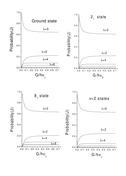
Figure 5: Occupation probabilities of the different $\lambda$ bosons as function of the scaled strength parameter $G/h\nu 2$ for a calculation that includes all even values of $\lambda$ up to 8. The lines are labelled by $\lambda$.

In Fig. 6 we show the energy ratios obtained for the ground state band when we consider only S and D bosons. In this case there are not free parameters (except for the pairing strength) and it is quite clear that we are not able to reproduce a rotational band.

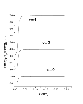
Figure 6: Ratio of the energies of the states with seniority $\nu$ to the energy of the $2_{1}$ state (corresponding to seniority one) as function of the scaled strength parameter $G/h\nu_{2}$ for a calculation that includes only S and D bosons.

The main weakness for the relevance of the present calculation is related to how well is taken into account the Pauli Principle by our model hamiltonian. In a Nilsson like calculation one has two main ingredients: on the one side the quadrupole-quadrupole interaction deforms the systems, whose ground sate can be written as a condensate of a boson that if formed by S, D, G, etc. bosons with well-defined probabilities [9, 13] and then one must consider the pairing interaction, that change by a small amount these probabilities. The contribution due to the pairing interaction between fermions can be taken into account using Pauli violating diagrams[9, 13]. The diagrams that appear in this treatment are similar to the ones generated by our model hamiltonian, but they do not have constant matrix elements. The fact that one obtains a rotational spectra, when using a large space, is an indication that the replacement of the correct matrix element by a constant may not be a bad approximation.

We can now go on to the main conclusion of the present paper. The S and D bosons used in the IBA model [2, 3] are different from the ones that appears in a quadrupole-quadrupole+pairing (Nilsson like) calculation. Using our model hamiltonian we have shown that one cannot ignore the importance of the high angular momentum bosons in the description of the ground sate rotational band, even if the occupation probabilities of these bosons are very small. Our result suggests that the S and D bosons used in the IBA are not directly related to the ones obtained in a Nilsson+BCS treatment. The S and D dominance obtained is a manifestation of a general effect found in Ref. [17], but the small amplitudes of the “bosons” with large angular momentum are essential to obtain a good description of the ground state rotational band.

Valuable discussions with J. Dukelsky related to the work reported herein are gratefully acknowledged.

This work was supported in part by the grant UBA-CYT x-204, x-053 and from CONICET PIP02618/00 as well as from Carrera del Investigador Científico y Técnico.

IV Appendix 1

The single j shell

An attractive pairing-interaction between fermions in a single j-shell has a well known exact solution that for the seniority zero states is expressed in terms of the number of pairs of particles (N) and the degeneracy ($\Omega=j+\frac{1}{2})$ as

$$E(N)=-|G|N\Omega\left(1-\frac{(N-1)}{\Omega}\right).$$ (13)

The second term can be considered to arise from the Pauli principle between the pairs of fermions, each having an energy $-|G|\Omega$.

In the case of S bosons the repulsive pairing hamiltonian is written as ($G>0$)

$$H_{P}=W_{s}S^{\dagger}S+GS^{\dagger}S^{\dagger}SS,$$ (14)

and it is diagonal in the states of N bosons, yielding for the energy

$$E(N)=W_{s}N+GN(N-1)=W_{s}N\left(1+\frac{G(N-1)}{W_{s}}\right).$$ (15)

To relate this result with the fermionic case one must use $W_{s}=-|G|\Omega$ and then both energies coincide.

References

- [1] J. Dukelsky and S. Pittel , Phys. Rev. Lett.86, 4791, 2001.
- [2] A. Arima and F. Iachello, Ann. Phys., NY 99, 253, 1976.
- [3] A. Arima and F. Iachello, Ann. Phys., NY 111, 20, 1978.
- [4] T. Otsuka, Nucl. Phys. A368, 244, 1981.
- [5] M. R. Zirnbauer and D. M. Brink, Nucl. Phys. A 384, 1, 1982.
- [6] C. Bloch and A. Messiah, Nucl. Phys. 9, 95, 1962.
- [7] A. L. Goodman, Advances in Nuclear Structure, Vol. 11 (ed. J.W. Negele and E. Vogt, NY, Plenum)
- [8] T. Otsuka, A. Arima and N. Yoshinaga, Phys. Rev. Lett. 48, 387, 1982.
- [9] J. Dukelsky, G. G. Dussel and H. M. Sofia, Nucl. Phys. A373, 267, 1982.
- [10] A. Bohr and B. Mottelson, Phys. Scr. 22, 468, 1980.
- [11] D. R. Bes, R. A. Broglia, E. Maglione and A. Vitturi, Phys. Rev. Lett. 48, 1001, 1982.
- [12] E. Maglione, A. Vitturi, C. A. Dasso R. A. Broglia, Nucl. Phys. A404, 333,1983.
- [13] J. Dukelsky, G. G. Dussel and H. M. Sofia, J. Phys. G: Nucl. Phys. 11, L91, 1985.
- [14] J. Dukelsky, C. Esebbag, and P. Schuck, Phys. Rev. Lett. 87, 066403 (2001).
- [15] F. Pan, L-R. Dai, Y-A. Luo and J. P. Draayer, Phys. Rev. C 68, 014308 (2003).
- [16] J. Dukelsky, S. Pittel and G. Sierra, submitted to Reviews of Modern Physics (2003).
- [17] R. W. Richardson, Phys. Lett. 3, 277 (1963).
- [18] D. R. Bes, Nucl. Phys. 10, 373 (1959).
- [19] R. W. Richardson, J. Math. Phys. 9, 1327, (1968).