MKPH-T-04-06
Interaction effects in ${\bm{K}^{+}}$ photoproduction on the deuteron

Abstract

Kaon photoproduction on the deuteron is studied with respect to a specific two-body contribution, namely a pion mediated production process, besides other final state interaction contributions from kaon-nucleon and hyperon-nucleon scattering. In this process, a pion is first photoproduced on one nucleon and then interacts with the spectator nucleon in a strangeness exchange reaction leading to a kaon and a hyperon. A sizeable effect from this pion mediated contribution is found, considerably larger than the previously studied hyperon-nucleon rescattering, whereas kaon-nucleon rescattering is much less important. Besides total and semi-inclusive differential cross sections, tensor target asymmetries are studied with respect to the influence of such interaction effects.

I Introduction

The study of kaon photoproduction has drawn attention for more than three decades since the work of Thom Tho66 , who analyzed the reaction $\gamma$p$\rightarrow$K${}^{+}\Lambda$ by using Feynman diagrams for the Born terms and partial wave amplitudes for the resonances. Adelseck et al. AdB85 evaluated the resonance terms using diagrammatic techniques, in order to ensure the relativistic invariance of the operator. The advent of a new generation of high duty-factor accelerators of sufficiently high energy such as MAMI in Mainz, ELSA in Bonn, or CEBAF in Newport News, has triggered several new analyses. David et al. DaF96 have analyzed the strangeness production by including in addition spin-5/2 resonances and off-shell effects of the resonance vertices. Mart and Bennhold Mar96 ; BeM96 have included an overall hadronic form factor in the production operator. This work was refined in Mar00 ; LeM01 by allowing different hadronic form factors at the various vertices in conjunction with the recipe of Haberzettl HaB98 in order to ensure gauge invariance. Other models were used in HaC01 investigating pseudovector coupling and in JaR02 studying the role of hyperon resonances in kaon photoproduction off the nucleon.

The channels mostly investigated in kaon photoproduction are the proton channels, $\gamma p\rightarrow K^{+}\Lambda$ and $\gamma p\rightarrow K^{+}\Sigma^{0}$, in view of a relatively large number of experimental data for these channels Boc94 ; Tra98 . Because the neutron has a short lifetime, free neutron targets are not available for the study of the neutron channels, and thus one uses light nuclei like deuterium or ³He as effective neutron targets. The deuteron is particularly suited because of its small binding energy and its simple structure. With the purpose to extract the elementary cross section on a neutron target, Li et al. LiW92 have calculated the reactions $\gamma d\rightarrow K^{0}\Lambda p$, $\gamma d\rightarrow K^{0}\Sigma^{0}p$, and $\gamma d\rightarrow K^{+}\Sigma^{-}p$ in the impulse approximation (IA) only. They concluded that the deuteron can be used to study K⁰ and K⁺ photoproduction from the neutron. The study of the hyperon-nucleon interaction is another important aspect of of kaon photoproduction on the deuteron. Several investigations of this question exist already. Renard and Renard ReR67a ; ReR67b have derived the formalism and studied the $\Lambda n$ interaction in kaon photoproduction off the deuteron. Adelseck and Wright AdW89 have examined the $\Lambda n$ final state interaction in kaon photoproduction from the deuteron via a distorted wave formalism by using a simple $\Lambda n$ potential. With the intention of investigating the hyperon-nucleon interaction, in a recent paper Yamamura et al. YaM99 have calculated the hyperon-nucleon final state interaction for the K⁺ channels by using the more realistic Nijmegen $YN$ potential from MaR89 ; RiS99 . They found sizeable effects in both, exclusive as well as inclusive cross sections from the $YN$ interaction, in particular a cusplike structure near the production threshold of the $\Sigma$ channels, and concluded that precise data would allow to study the $YN$ interaction in greater detail. Another recent calculation is from Kerbikov Ker01 who also investigated the hyperon-nucleon final state interaction.

Thus up to now, of the various interactions in the final three-particle state of kaon photoproduction on the deuteron, most of the calculations have considered only the hyperon-nucleon final state interaction ($YN$-FSI) quantitatively. With respect to the other two possible interactions in the kaon-hyperon and kaon-nucleon two-body subsystems, the former is usually assumed to be already included in the elementary production amplitude whereas the latter has been considered as negligible. In the present paper, our first point of interest is the quantitative study of this kaon-nucleon final state interaction ($KN$-FSI) by including the kaon-nucleon scattering matrix into the photoproduction amplitude. Our second point refers to the inclusion of another competing two-body process which might give in addition an important contribution and which has been neglected hitherto. It refers to the pion mediated kaon production process, denoted by “$\pi\rightarrow K$”, in which the absorbed photon produces first on one nucleon a pion which then interacts with the specator nucleon via a strangeness exchange reaction leading to a kaon and a hyperon. Although on first sight this process, being a two-step reaction, is expected to be suppressed, it could give a sizeable contribution in view of the fact that the pion photopoduction cross section is still relatively strong in the region of kaon photoproduction. For both hadronic reactions, $KN$ scattering and $\pi\rightarrow K$, separable potentials are used. After completion of this work, a very recent study of two-body contributions to the photoproduction operator was published by Maxwell Max04 using a diagrammatic approach where the pion mediated process is included in lowest order. Our approach differs with respect to the one-body photoproduction operator on the nucleon and with respect to a complete inclusion of the various two-body reactions in the two-body subsystems. In particular, final state correlations like hyperon-nucleon and kaon-nucleon rescattering were not included in Max04 .

In Sect. II, we briefly review the formal aspects of the various two-body elementary reactions which we include in our treatment of kaon photoproduction on the deuteron. In Sect. III, the formalism for calculating the transition matrix and cross section for kaon photoproduction on the deuteron with inclusion of final state interactions and the $\pi\rightarrow K$ process is given. The results are presented in Sect. IV and we close with some conclusions and an outlook in Sect. V. Throughout the paper we use natural units $\hbar=c=1$.

II Elementary reactions

Kaon photoproduction on the deuteron is governed by basic two-body processes, namely meson photoproduction on a nucleon and hadronic two-body scattering reactions. In this section we will collect the necessary ingredients for the various processes which we have included in the present theoretical description of kaon photoproduction on the deuteron.

The general form of these elementary two-body reactions is

$${A}(p_{A})+{B}(p_{B}) \rightarrow {C}(p_{C})+{D}(p_{D})\,,$$ (1)

where $p_{i}=(E_{i},\,\vec{p}_{i})$ denotes the 4-momentum of particle “$i$” with $i\in\{A,B,C,D\}$. Particles $A$ and $B$ stand for a photon and a nucleon in photoproduction, a meson and a baryon in the case of kaon-nucleon scattering and the $\pi N\rightarrow KY$ process, or a pair of baryons like in hyperon-nucleon scattering. Corresponding assignments stand for the final particles $C$ and $D$.

In order to compare the theoretical predictions for the various elementary reactions with experimental data one has to evaluate the corresponding cross sections. Following the conventions of Bjorken and Drell BjD64 the general form for the differential cross section of a two-particle reaction in the center of mass system is given by

$$\frac{d\sigma}{d\Omega_{C}} = \frac{1}{(2\pi W)^{2}}\,\frac{p_{C}\,F}{p_{A}\,s}\sum_{\mu_{D}\mu_{C}\mu_{B}\mu_{A}}\left|{\cal M}_{\mu_{D}\mu_{C}\mu_{B}\mu_{A}}(\vec{p}_{D},\vec{p}_{C},\vec{p}_{B},\vec{p}_{A})\right|^{2}$$ (2)

with ${\cal M}_{\mu_{D}\mu_{C}\mu_{B}\mu_{A}}$ as reaction matrix, $\mu_{i}$ denoting the spin projection of particle “$i$” on some quantization axis, and

$$F = \frac{E_{A}E_{B}E_{C}E_{D}}{F_{A}F_{B}F_{C}F_{D}}\,,$$ (3)

where $F_{i}$ is a factor arising from the covariant normalization of the states and its form depends on whether the particle is a boson ($F_{i}=2E_{i}$) or a fermion ($F_{i}=E_{i}/m_{i}$), where $E_{i}$ and $m_{i}$ are its energy and mass, respectively. The factor $s=(2s_{A}+1)(2s_{B}+1)$ takes into account the averaging over the initial spin states, where $s_{A}$ and $s_{B}$ denote the spins of the incoming particles $A$ and B, respectively. If $A$ stands for a photon then $s_{A}=1/2$. Note that $p_{C}$ means $|\vec{p}_{C}|$. All momenta are functions of the invariant mass of the two-body system $W$, i.e. $p_{i}=p_{i}(W)$.

For the scattering processes, it is more convenient to use non-covariant normalization of the states and to switch to a coupled spin representation replacing the ${\cal M}$-matrix by the ${\cal T}$-matrix via

$${\cal M}^{fi}_{\mu_{D}\mu_{C}\mu_{B}\mu_{A}}(\vec{p}_{D},\vec{p}_{C},\vec{p}_{B},\vec{p}_{A}) = (2\pi)^{3}\sqrt{F_{A}F_{B}F_{C}F_{D}}\sum_{S^{\prime}\mu^{\prime}_{S^{\prime}}S\mu_{S}}C^{s_{C}s_{D}S^{\prime}}_{\mu_{C}\mu_{D}\mu^{\prime}_{S^{\prime}}}\,C^{s_{A}s_{B}S}_{\mu_{A}\mu_{B}\mu_{S}}\,{\cal T}^{fi}_{S^{\prime}\mu^{\prime}_{S^{\prime}}S\mu_{S}}(\vec{p}_{D},\vec{p}_{C},\vec{p}_{B},\vec{p}_{A})\,,$$ (4)

with $C^{s_{C}s_{D}S^{\prime}}_{\mu_{C}\mu_{D}\mu^{\prime}_{S^{\prime}}}$ as approriate Clebsch-Gordan coefficient. As next step we introduce a partial wave representation of the ${\cal T}$-matrix which reads with $\vec{p}^{\,\prime}$ and $\vec{p}$ as the final and initial relative momenta, respectively,

$${\cal T}^{fi}_{S^{\prime}\mu^{\prime}_{S^{\prime}}S\mu_{S}}(W,\vec{p}^{\,\prime},\vec{p}\,) = \sum_{\ell^{\prime}\ell J}X^{\ell^{\prime}\ell J}_{S^{\prime}\mu^{\prime}_{S^{\prime}}S\mu_{S}}(\hat{p}^{\prime},\hat{p})\,T^{\ell^{\prime}\ell J}_{fi}(W,p^{\prime},p)\,,$$ (5)

where we have introduced

$$X^{\ell^{\prime}\ell J}_{S^{\prime}\mu^{\prime}_{S^{\prime}}S\mu_{S}}(\hat{p}^{\prime},\hat{p}) = \sum_{\mu^{\prime}_{\ell^{\prime}}\mu_{\ell}\mu_{J}}Y_{\ell^{\prime}\mu^{\prime}_{\ell^{\prime}}}(\hat{p}^{\prime})\,Y_{\ell\mu_{\ell}}^{\ast}(\hat{p})\,C^{\ell^{\prime}S^{\prime}J}_{\mu^{\prime}_{\ell^{\prime}}\mu^{\prime}_{S^{\prime}}\mu_{J}}\,C^{\ell SJ}_{\mu_{\ell}\mu_{S}\mu_{J}}\,.$$ (6)

Here $\ell$ and $J$ denote the orbital and total angular momenta of the system, respectively, $Y_{\ell\mu}(\hat{p})$ a spherical harmonics, and $\hat{p}=(\theta_{\vec{p}},\phi_{\vec{p}})$. The partial wave ${\cal T}$-matrix is obtained as solution of the Lippmann-Schwinger equation

$${\cal T}^{\ell^{\prime}\ell J}_{fi}(W,p^{\prime},p) = V^{\ell^{\prime}\ell J}_{fi}(p^{\prime},p)+\sum_{n\ell^{\prime\prime}}2m_{n}\int_{0}^{\infty}dp^{\prime\prime}_{n}~{}(p^{\prime\prime}_{n})^{2}\,\frac{V^{\ell^{\prime}\ell^{\prime\prime}J}_{fn}(p^{\prime},p^{\prime\prime}_{n})\,T^{\ell^{\prime\prime}\ell J}_{ni}(W,p^{\prime\prime}_{n},p)}{q_{n}^{2}-(p^{\prime\prime}_{n})^{2}+i\varepsilon}\,,$$ (7)

where “$n$” labels possible intermediate two-particle configurations with total mass $M_{n}$, reduced mass $m_{n}$, and with relative momentum

$$q_{n} = \sqrt{2m_{n}\left(W-M_{n}\right)}$$ (8)

in the c.m. system. Now we will briefly review the different elementary processes in some detail.

II.1 Kaon photoproduction on the nucleon

In the simplest approach to kaon photoproduction on the nucleon, one approximates the production amplitude ${\cal M}$ with the tree-level diagrams shown in Fig. 1. In principle these diagrams serve as driving terms in a system of coupled equations in which hadronic rescattering is included which is important in order to ensure unitarity. However, in the present work we use the simpler model of Lee et al. LeM01 , called isobar model, in which all diagrams of Fig. 1 are taken into account except the Y^∗-pole diagram (e). In the Born terms pseudoscalar coupling is used for the hadronic meson-baryon vertices. As resonances are included for the N^∗-pole (diagram (d)) S₁₁(1650), P₁₁(1710), S₃₁(1900), P₃₁(1910), and P₁₃(1720) and for the K^∗-pole (diagram (f)) K^∗(892) and K₁(1270). Separate hadronic form factors for each vertex were used which, however, destroys gauge invariance. In order to restore gauge invariance, a recipe from Haberzettl HaB98 was utilized.

Figure 1: Elementary diagrams of kaon photoproduction on the nucleon. Born terms (a) - (c): nucleon, hyperon and kaon poles, respectively; resonance terms (d) - (f): nucleon, hyperon, and kaon resonance poles, respectively.

The photoproduction amplitude ${\cal M}^{K\gamma N}$ is parametrized usually in terms of four invariant operators $\Gamma^{i}_{\lambda}$, accompanied by invariant amplitudes $A_{i}^{K\gamma N}$ which are functions of the Mandelstam variables only. Thus the amplitude has the form

$${\cal M}^{K\gamma N}_{\mu_{Y}\mu_{N}\lambda} = \bar{u}_{\mu_{Y}}\Big{(}\sum_{i=1}^{4}A_{i}^{K\gamma N}\Gamma^{i}_{\lambda}\Big{)}u_{\mu_{N}}\,,$$ (9)

where we have suppressed the dependence on the kinematical variables. The hyperon and nucleon Dirac spinors are denoted by $u_{\mu_{Y}}$ and $u_{\mu_{N}}$, respectively. The invariant Dirac operators $\Gamma_{i}$ are gauge invariant Lorentz pseudoscalars and given in terms of the usual $\gamma$-matrices, the photon momentum $k$, its polarization vector $\epsilon_{\lambda}$, where $\lambda$ labels the polarization states, the meson momentum $q$ and $P=(p^{\prime}+p)/2$, where $p$ and $p^{\prime}$ denote initial and final baryon momenta, respectively Don72 ,

$$\Gamma^{1}_{\lambda} = {\textstyle\frac{1}{2}}\gamma_{5}\left({\epsilon\!\!/}\!_{\lambda}k\!\!\!/-k\!\!\!/{\epsilon\!\!/}\!_{\lambda}\right)\,,$$ (10)

$$\Gamma^{2}_{\lambda} = \gamma_{5}\left[(2q-k)\cdot\epsilon_{\lambda}P\cdot k-(2q-k)\cdot kP\cdot\epsilon_{\lambda}\right]\,,$$ (11)

$$\Gamma^{3}_{\lambda} = \gamma_{5}\left(q\cdot k{\epsilon\!\!/}\!_{\lambda}-q\cdot\epsilon_{\lambda}k\!\!\!/\right)\,,$$ (12)

$$\Gamma^{4}_{\lambda} = i\epsilon_{\mu\nu\rho\sigma}\gamma^{\mu}q^{\nu}\epsilon^{\rho}_{\lambda}k^{\sigma}\,.$$ (13)

The contributions of the various diagrams in Fig. 1 to the invariant amplitudes is straightforward and explicit expressions are listed in Sal03 .

The coupling constants and cut-off parameters were determined by a fit to the experimental data. Fig. 2 shows the total cross section for the various channels as obtained from this model together with experimental data Tra98 ; Goe99 and with its older version BeM96 . One readily notes that the new model describes the data for $\gamma p\rightarrow K^{+}\Sigma^{0}$ slightly better than the old one and considerably better for $\gamma{p}\rightarrow{K}^{0}\Sigma^{+}$. However, the prediction for the channel $\gamma{n}\rightarrow{K}^{0}\Lambda$ appears unrealistically large. The authors of LeM01 explain this feature by the lack of experimental data in that channel making the parameter fitting uncontrollable. It may well be that the older model may give a more realistic description for this channel. Nevertheless, we use the new model in the present work.

Figure 2: Total cross sections of kaon photoproduction on the nucleon versus photon lab energy. Solid curves: the model of LeM01 ; dashed curves: model of BeM96 ; experimental data from the SAPHIR collaboration Tra98 ; Goe99 .

II.2 Pion photoproduction on the nucleon

For pion photoproduction on the nucleon we use the MAID model DrH99 . The model contains Born terms (diagram (a)-(c),(e) of Fig. 3), vector mesons $\rho$ and $\omega$ (diagram (f)), and a series of nucleon resonances $P_{33}(1232)$, $P_{11}(1440)$, $D_{13}(1520)$, $S_{11}(1535)$, $F_{15}(1680)$, and $D_{33}(1700)$ (diagram (d)). For the Born terms, this model uses both pseudoscalar and pseudovector coupling with a gradual transition from pure pseudovector coupling at threshold to pure pseudoscalar coupling at high photon energies. This operator has been developed for photon energies up to 1.6 GeV which is above the threshold of kaon photoproduction and, therefore, can be used for the evaluation of the pion mediated reaction on the deuteron.

Figure 3: Elementary diagrams for pion photoproduction on the nucleon. Born terms: (a) - (c) nucleon, crossed nucleon and pion poles and (e) Kroll-Rudermann contact term; (d): resonance term; (f): vector meson exchange.

Figure 4: Total cross sections of pion photoproduction on the nucleon versus photon lab energy from MAID DrH99 .

The resulting total cross sections are shown in Fig. 4. Comparing Fig. 2 with Fig. 4, one clearly notes that the cross section for pion photoproduction on the nucleon of about 25 $\mu$b around $E_{\gamma}=1.6$ MeV is still much stronger (about 10 times) than the cross section for kaon photoproduction at the same energies. This fact indicates that the pion mediated photoproduction contribution may have a sizeable influence on kaon photoproduction on the deuteron.

The MAID-operator is given in the photon-pion c.m. system in terms of the CGLN-amplitudes $F_{1}$ through $F_{4}$ ChG57

$${\cal M}^{\gamma\pi N}_{\mu_{N}^{\prime}\mu_{N}\lambda} = \chi_{\mu_{N}^{\prime}}^{\dagger}(\vec{\sigma}\cdot\vec{\epsilon}_{\lambda}\,F_{1}-i\vec{\sigma}\cdot\hat{q}\,\vec{\sigma}\cdot\hat{k}\times\vec{\epsilon}_{\lambda}\,F_{2}+\vec{\sigma}\cdot\hat{k}\,\hat{q}\cdot\vec{\epsilon}_{\lambda}\,F_{3}+\vec{\sigma}\cdot\hat{q}\,\hat{q}\cdot\vec{\epsilon}_{\lambda}\,F_{4})\chi_{\mu_{N}}\,,$$ (14)

where $\hat{a}$ means a unit vector in the direction of $\vec{a}$, $\vec{\sigma}$ denotes the nucleon spin operator. The $F_{i}$ amplitudes are functions of the invariant mass $W$ and the relative c.m. angle $\theta$ between photon and pion momentum. Since, however, we need the amplitude in a general frame of reference for the process on the deuteron, we have to establish a relation connecting the $F_{i}$ amplitudes, defined in the c.m. system, to the invariant amplitudes $A_{i}^{\pi\gamma}$, defined in analogy to Eq. (9), in any system. Comparing the two representations, one finds as desired relation

$$\left(\begin{array}[]{c}A^{\gamma\pi N}_{1}\\ A^{\gamma\pi N}_{2}\\ A^{\gamma\pi N}_{3}\\ A^{\gamma\pi N}_{4}\end{array}\right) = 4\pi\left(\begin{array}[]{cccc}W^{+}&-W^{-}&-2m_{N}\frac{q\cdot k}{W^{-}}&2m_{N}\frac{q\cdot k}{W^{+}}\\ 0&0&1&-1\\ 1&1&-W^{+}\frac{q\cdot k}{W^{-}}&-W^{-}\frac{q\cdot k}{W^{+}}\\ 1&1&-\frac{q\cdot k}{W^{-}}&-\frac{q\cdot k}{W^{+}}\end{array}\right)\left(\begin{array}[]{c}\frac{1}{\sqrt{E_{N}^{\prime\,+}E_{N}^{+}}}\frac{1}{W^{-}}F_{1}\\ \frac{1}{\sqrt{E_{N}^{\prime\,-}E_{N}^{-}}}\frac{1}{W^{+}}F_{2}\\ \frac{1}{qk}\sqrt{\frac{E_{N}^{+}}{E_{N}^{\prime\,+}}}\frac{1}{W^{+}}F_{3}\\ \frac{1}{qk}\sqrt{\frac{E_{N}^{-}}{E_{N}^{\prime\,-}}}\frac{1}{W^{-}}F_{4}\end{array}\right)\,,$$ (27)

where we have introduced the notation $W^{\pm}=W\pm m_{N}$ and analogously for $E_{N}^{\pm}$ and $E_{N}^{\prime\,\pm}$. We would like to point out that the notation $q$ and $k$ in Eq. (27) means the absolute value of three-vectors whereas $q\cdot k$ refers to the 4-vector scalar product. With these relations, we can evaluate ${\cal M}^{\gamma\pi N}$ in any frame because of the invariant character of the $A^{\gamma\pi N}_{i}$.

II.3 Hyperon-nucleon scattering

For hyperon-nucleon scattering we use the Nijmegen interaction potential $V_{YN}$ from MaR89 ; RiS99 . This interaction is described in terms of one-boson exchanges. Since the hyperon is a baryon with strangeness $S=-1$, the exchanges contain both strange and non-strange mesons. The basic diagrams of this model are displayed in Fig. 5.

Figure 5: Boson exchange diagrams of the hyperon-nucleon potential $V_{YN}$. The left diagram describes a strangeness exchange and the right one a non-strangeness exchange.

Three types of mesons are considered, pseudoscalar, scalar, and vector mesons. The pseudoscalars are $\pi$, $\eta$, $\eta^{\prime}$, and K with an $\eta-\eta^{\prime}$ mixing angle $\theta_{P}=-23.0^{\circ}$ from the Gell-Mann-Okubo mass formula. As vector mesons are included $\rho$, $\phi$, K^∗, and $\omega$ with an ideal $\phi-\omega$ mixing angle $\theta_{V}=37.56^{\circ}$ and as scalar mesons $\delta$, $S^{*}$, $\kappa$, and $\varepsilon$ with a free $S^{*}-\varepsilon$ mixing angle to be determined in a fit to the $YN$ scattering data. Also included are contributions from Pomeron, $f$, $f^{\prime}$, and $A_{2}$ exchanges. For details we refer to MaR89 ; RiS99 .

II.4 Kaon-nucleon scattering

In order to estimate the supposedly smaller influence of kaon-nucleon rescattering, we take a simple rank-one separable interaction potential for which the partial wave representation reads

$$V_{KN}^{\ell J}(p^{\prime},p) = \lambda^{\ell J}_{KN}\,g^{\ell J}_{KN}(p^{\prime})\,g^{\ell J}_{KN}(p)\,,$$ (28)

where $\lambda^{\ell J}_{KN}=\pm 1$ is a phase parameter and $g^{\ell J}_{KN}(p)$ is a form factor. It is taken in the form

$$g^{\ell J}_{KN}(p) = \frac{B^{\ell J}_{KN}\,p^{\ell}}{\left[p^{2}+(A^{\ell J}_{KN})^{2}\right]^{\frac{\ell+2}{2}}}\,,$$ (29)

where $B^{\ell J}_{KN}$ and $A^{\ell J}_{KN}$ are parameters which characterize strength and range of the potential.

Table 1: Parameters of the separable potential of rank-1 for kaon-nucleon scattering.

partial wave	I	$\lambda$	$A^{\ell J}$ [MeV]	$B^{\ell J}$ [MeV]
$S_{01}$	0	+	617.56	431.84
$P_{01}$	0	$-$	908.53	1815.2
$P_{03}$	0	+	353.27	204.55
$D_{03}$	0	$-$	513.34	572.94
$S_{11}$	1	+	763.32	1049.9
$P_{11}$	1	+	547.25	630.43
$P_{13}$	1	$-$	569.42	471.68
$D_{13}$	1	+	1256.0	4979.8

With this potential, the Lippmann-Schwinger equation for the partial wave ${\cal T}$-matrix reads

$${\cal T}^{\ell J}_{KN}(W;p^{\prime},p) = \lambda^{\ell J}_{KN}\,g^{\ell J}_{KN}(p^{\prime})\,\left(g^{\ell J}_{KN}(p)+2m_{KN}\int_{0}^{\infty}dp^{\prime\prime}\,(p^{\prime\prime})^{2}\,\frac{g^{\ell J}_{KN}(p^{\prime\prime})\,T^{\ell J}_{KN}(W,p^{\prime\prime},p)}{q^{2}-(p^{\prime\prime})^{2}+i\varepsilon}\right),$$ (30)

which can be solved analytically yielding

$$T^{\ell J}_{KN}(W,p^{\prime},p) = \frac{\lambda^{\ell J}_{KN}\,g^{\ell J}_{KN}(p^{\prime})\,g^{\ell J}_{KN}(p)}{1-2\,m_{KN}\,\lambda^{\ell J}_{KN}\int_{0}^{\infty}dp^{\prime\prime}\,(p^{\prime\prime})^{2}\,\frac{\left(g^{\ell J}_{KN}(p^{\prime\prime})\right)^{2}}{q^{2}-(p^{\prime\prime})^{2}+i\varepsilon}}\,.$$ (31)

For $\ell=0$ one finds explicitly

$${\cal T}^{0J}_{KN}(p^{\prime},p) = \frac{\lambda^{0J}_{KN}\,(B^{0J}_{KN})^{2}}{\left[(p^{\prime})^{2}+(A^{0J}_{KN})^{2}\right]\left[p^{2}+(A^{0J}_{KN})^{2}\right]}\left[1+\frac{\pi m(B^{0J}_{KN})^{2}}{2A^{0J}_{KN}\left[A^{0J}_{KN}-iq\right]^{2}}\right]^{-1},$$ (32)

where the parameters of the potential are determined by fitting the $(\ell=0)$-phase shifts to experimental data. The results for the phase shifts are shown in Fig. 6 together with the phase shifts of the SAID-analysis HyA92 based on experimental data. The resulting parameters of this fit are listed in Table 1.

Figure 6: Phase shifts of kaon-nucleon scattering versus kaon lab momentum. Solid curves: results for a separable potential of rank-1; triangles: phase shifts from the SAID-analysis HyA92 .

Figure 7: Total elastic cross sections of various channels for kaon-nucleon scattering versus kaon lab momentum. Curves: predictions using the separable potential of rank-1; experimental data from Cam74 ; Abe75 . Notation S₁ means S₀₁+S₁₁ and similarly for P₁, P₃ and D₃.

Fig. 6 shows that the separable potential of rank-1 describes most of the phase shifts fairly well. The best fit is achieved for the partial wave D₁₃ because of its simple form. Relatively good fits are also obtained for S₁₁, P₀₁, P₁₁, and P₀₃. The oscillatory form of D₀₃ and S₀₁ and the relatively sharp peak of P₁₃ can not be fitted well by this simple separable potential. However, for the present study of the influence of $KN$ rescattering this fit is good enough.

The total elastic cross sections of kaon-nucleon scattering with the increasing contribution of partial waves are shown in Fig. 7. The left panel (a) shows the cross section for $K^{+}p\rightarrow K^{+}p$ having total isospin $I=1$. The middle and right panels (b) and (c) show the cross sections for channels having contributions from both total isospins $I=1$ and $I=0$, i.e. $K^{+}n\rightarrow K^{+}n$ (panel (b)) and $K^{+}n\rightarrow K^{0}p$ (panel (c)). For the reaction $K^{+}p\rightarrow K^{+}p$ (panel (a)) a reasonable agreement with the data from Cam74 ; Abe75 is achieved by including S- and P-waves only. D-waves show some effect above kaon momenta $p_{K}\approx 1.6$ GeV/c.

II.5 The $\pi N\rightarrow KY$ process

The interaction $\pi N\rightarrow KY$ couples the $\pi N$-channel with the $KY$-channel and thus one deals with a coupled two-channel problem. Therefore, the potential and the reaction matrix are described by $2\times 2$-matrices. Again we take for simplicity a separable interaction potential, which reads in this case

$$V_{KY,\pi N}(p^{\prime},p)=\lambda g(p^{\prime})_{KY,\pi N}\,g_{KY,\pi N}^{\dagger}(p)\,,$$ (33)

where

$$g_{KY,\pi N}(p)=\left(\begin{array}[]{c}g_{\pi N}(p)\\ g_{KY}(p)\\ \end{array}\right)$$ (34)

with an analogous functional form for $g_{\pi N}(p)$ and $g_{KY}(p)$ as in (29).

Table 2: Parameters of the separable potential of rank-1 for the reaction $\pi N$ $\rightarrow$ KY with S-waves only.

channel	partial wave	$\lambda$	$A^{\ell J}$ [MeV]	$B^{\ell J}$ [MeV]
$\pi N$	$S_{11}$	+	1039.6	559.03
$\pi N$	$S_{31}$	+	140.97	108.94
$KY$	$S_{11}$	+	179.39	148.80
$KY$	$S_{31}$	+	115.80	224.41

Figure 8: Total cross sections of various channels for the $\pi N$$\rightarrow$KY process versus pion lab-momentum. Solid curves: calculations using a separable potential of rank-1 only in S-waves; triangles: experimental data taken from Kna75 ; Sax79 ; Bak78 ; Har79 ; Can83 ; Goo69 ; Dah67 .

The same steps like in kaon-nucleon scattering lead to the final form of the separable $T$-matrix

$${\cal T}_{KY,\pi N}^{\ell J}(p^{\prime},p) = \lambda\,g_{KY,\pi N}^{\ell J}(p^{\prime})\,(g^{\ell J}(p))_{KY,\pi N}^{\dagger}\left[1-2\,\lambda\int_{0}^{\infty}dp^{\prime\prime}\,(p^{\prime\prime})^{2}\sum_{n\in\{\pi N,KY\}}m_{n}\frac{\left(g^{\ell J}_{n}(p^{\prime\prime})\right)^{2}}{q_{n}^{2}-(p^{\prime\prime})^{2}+i\varepsilon}\right]^{-1}\,.$$ (35)

For $\ell=0$ the $\pi N\rightarrow KY$ transition amplitude is given by

$${\cal T}_{KY,\pi N}^{0J}(p^{\prime},p) = \frac{B^{0J}_{\pi N}B^{0J}_{KY}}{\left[(p^{\prime})^{2}+(A^{0J}_{\pi N})^{2}\right]\left[p^{2}+(A^{0J}_{KY})^{2}\right]}\left[1+\pi\sum_{n\in\{\pi N,KY\}}\frac{m_{n}(B^{0J}_{n})^{2}}{2A^{0J}_{n}\left[A^{0J}_{n}-iq_{n}\right]^{2}}\right]^{-1}\,.$$ (36)

The parameters of the transition potential, listed in Table 2, are determined by fitting the cross section $\pi N\rightarrow KY$ to experimental data.

The total cross sections for the reaction $\pi N$ $\rightarrow$ KY are shown in Fig. 8. Panels (a) and (b) are for the $\Lambda$-channels and the others for the $\Sigma$-channels. The experimental data for channel $K^{0}\Lambda$ are taken from Kna75 ; Sax79 , for $K^{+}\Sigma^{+}$ from Can83 , for $K^{0}\Sigma^{0}$ from Bak78 ; Har79 , and for $K^{+}\Sigma^{-}$ from Goo69 ; Dah67 . The solid lines are obtained by fitting the cross sections calculated by using a separable potential of rank-1 to the available experimental data. In this fit we take into account only S-waves with total isospin $I=\frac{1}{2}$ and $I=\frac{3}{2}$, while the addition of D-waves does not improve the convergence with increasing kaon momentum. The resulting values of the potential parameters are given in Table 2.

In Fig. 8 it is seen that the separable potential of rank-1 with S-waves only can fit experimental data relatively well, especially in the channel $\pi^{-}$p $\rightarrow K^{0}\Lambda$. In this channel, the theoretical calculation underpredicts experimental data at kaon lab-momenta above about 1.6 GeV/c. This indicates that the higher partial waves become important in this energy region. Also it can be seen in the panel (c) that the separable potential of rank-1 with S-waves only cannot fit the data very well above about 1.6 GeV/c. However, as a reasonable approximation we keep only the S-waves in the calculation.

III Kaon photoproduction on the deuteron

Now we will turn to kaon photoproduction on the deuteron

$$\gamma(p_{\gamma})+{d}(p_{d}) \rightarrow {K}(p_{K})+{Y}(p_{Y})+{N}(p_{N})\,,$$ (37)

where $p_{\gamma}$, $p_{d}$, $p_{K}$, $p_{Y}$, and $p_{N}$ denote the 4-momenta of photon, deuteron, kaon, hyperon, and nucleon, respectively. We begin with a brief review of the general formalism for cross section and target asymmetries.

The general expression for the unpolarized cross section according to BjD64 is given by

$$d\sigma = \frac{\delta^{4}(p_{\gamma}+p_{d}-p_{K}-p_{Y}-p_{N})m_{N}m_{Y}d^{3}p_{N}d^{3}p_{Y}d^{3}p_{K}}{48(2\pi)^{5}|\vec{v}_{\gamma}-\vec{v}_{d}|E_{\gamma}E_{d}E_{N}E_{Y}E_{K}}\sum_{\mu_{Y}\mu_{N}\mu_{d}\lambda}\left|{\cal M}^{K\gamma d}_{\mu_{Y}\mu_{N}\mu_{d}\lambda}(\vec{p}_{Y},\vec{p}_{N},\vec{p}_{K},\vec{p}_{d},\vec{p}_{\gamma})\right|^{2}\,,$$ (38)

where $\mu_{Y}$, $\mu_{N}$, $\mu_{d}$, and $\lambda$ denote the spin projections of hyperon, nucleon, deuteron and the photon polarization, respectively. Covariant state normalization in the convention of BjD64 is assumed.

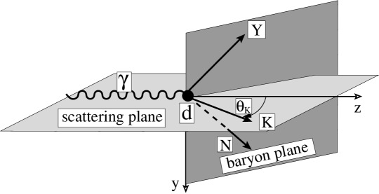
Figure 9: The kinematics of kaon photoproduction on the deuteron in the lab frame.

This expression is evaluated in the lab or deuteron rest frame. We have chosen a right-handed coordinate system where the $z$-axis is defined by the photon momentum $\vec{p}_{\gamma}$ and the $y$-axis by $\vec{p}_{\gamma}\times\vec{p}_{K}$. The kinematical situation is shown in Fig. 9. The scattering plane is defined by the momenta of photon $\vec{p}_{\gamma}$ and kaon $\vec{p}_{K}$ whereas the momenta of nucleon $\vec{p}_{N}$ and hyperon $\vec{p}_{Y}$ define the baryon plane. In this frame the kinematical variables of the initial state are

$$p_{d} = (M_{d},\,\vec{0})\quad\mbox{and}\quad p_{\gamma}=(p_{\gamma},\,p_{\gamma}\hat{z})\,.$$ (39)

The threshold lab energy is given by

$$p_{\gamma}^{thr}=\frac{(m_{YN}+m_{K})^{2}-m_{d}^{2}}{2m_{d}}\,,$$ (40)

where $m_{YN}=m_{Y}+m_{N}$. For the final state, we choose as independent variables the kaon three-momentum $\vec{p}_{K}=(p_{K},\theta_{K},\phi_{K})$, where we can choose $\phi_{K}=0$ since we do not consider polarized photons. Furthermore, the spherical angles $\Omega^{\,\ast}_{YN}=\hat{p}^{\,\ast}_{YN}=(\theta^{\,\ast}_{YN},\phi^{\,\ast}_{YN})$ of the relative $YN$-momentum $\vec{p}^{\,\ast}_{YN}=(\vec{p}^{\,\ast}_{Y}-\vec{p}^{\,\ast}_{N})/2$ in the $YN$-c.m. system as indicated by the asterisk. The relation to the corresponding lab frame quantities is obtained by an appropriate Lorentz boost with $\vec{\beta}=\vec{P}_{YN}/E_{YN}$, where

$$\vec{P}_{YN}=\vec{p}_{Y}+\vec{p}_{N}=\vec{p}_{\gamma}-\vec{p}_{K}\,,\quad\mbox{and}\quad E_{YN}=E_{Y}+E_{K}=E_{\gamma}+m_{d}-E_{K}\,.$$ (41)

The orientation of the baryon plane is characterized by $\Omega_{YN}$, the spherical angles of the relative $YN$-momentum in the lab system. For given photon energy and kaon emission angle $\theta_{K}$, the kaon momentum $p_{K}$ is bounded by $p_{K}^{min}\leq p_{K}\leq p_{K}^{max}$. In order to determine the boundaries we consider first the kaon momentum for a given invariant mass $W_{YN}=\sqrt{E_{YN}^{2}-\vec{P}_{YN}^{\,2}}$ of the $YN$-subsystem yielding two solutions

$$p_{K}=\frac{1}{2b}\,\Big{(}a\,p_{\gamma}\cos\theta_{K}\pm E_{\gamma d}\sqrt{a^{2}-4b^{2}m_{K}^{2}}\Big{)}\,,$$ (42)

where

$$a = W_{\gamma d}^{2}+m_{K}^{2}-W_{YN}^{2}\,,$$ (43)

$$b = W_{\gamma d}^{2}+p_{\gamma}^{2}\sin^{2}\theta_{K}\,,$$ (44)

$$W_{\gamma d}^{2} = E_{\gamma d}^{2}-p_{\gamma}^{2}=m_{d}(m_{d}+2\,p_{\gamma})\,,$$ (45)

$$E_{\gamma d} = m_{d}+p_{\gamma}\,.$$ (46)

The upper and lower limits of $p_{K}$ are determined by the minimal value of $W_{YN}^{2}$ which is $W_{YN}^{2}=m_{YN}^{2}$, resulting in

$$p_{K}^{max} = \frac{1}{2b}\,\Big{(}a_{0}\,p_{\gamma}\cos\theta_{K}+E_{\gamma d}\sqrt{a_{0}^{2}-4b^{2}m_{K}^{2}}\Big{)}\,,$$ (47)

$$p_{K}^{min} = \max\{0,\frac{1}{2b}\,\Big{(}a_{0}\,p_{\gamma}\cos\theta_{K}-E_{\gamma d}\sqrt{a_{0}^{2}-4b^{2}m_{K}^{2}}\Big{)}\}\,,$$ (48)

where $a_{0}=W_{\gamma d}^{2}+m_{K}^{2}-m_{YN}^{2}$. The lower limit $p_{K}=(a_{0}\,p_{\gamma}\cos\theta_{K}-E_{\gamma d}\sqrt{a_{0}^{2}-4b^{2}m_{K}^{2}})/2b>0$ applies if $0\leq\theta_{K}\leq\pi/2$ and, since $a_{0}>0$, if

$$a_{0}\,p_{\gamma}\cos\theta_{K}>E_{\gamma d}\sqrt{a_{0}^{2}-4b^{2}m_{K}^{2}}\,,$$ (49)

which happens for

$$p_{\gamma}>(m_{YN}^{2}-(m_{d}-m_{K})^{2})/(2(m_{d}-m_{K}))\,.$$ (50)

Integrating over the kaon momentum $p_{k}$ and over $\Omega^{\,\ast}_{YN}$, one obtains the semi-inclusive differential cross section of kaon photoproduction on the deuteron, where only the final kaon is detected without analyzing its energy,

$$\frac{d\sigma}{d\Omega_{K}} = \int_{p_{K}^{min}}^{p_{K}^{max}}dp_{K}\int d\Omega^{\,\ast}_{YN}\,\kappa\,\sum_{\mu_{Y}\mu_{N}\mu_{d}\lambda}\left|{\cal M}^{K\gamma d}_{\mu_{Y}\mu_{N}\mu_{d}\lambda}(\vec{p}_{YN},\,\vec{p}_{K},\,\vec{p}_{\gamma})\right|^{2}$$ (51)

with a kinematic factor

$$\kappa = \frac{m_{Y}m_{N}p_{K}^{2}p^{\,\ast}_{YN}}{24(2\pi)^{2}p_{\gamma}E_{K}W_{YN}}\,.$$ (52)

With respect to polarization observables, we consider only the tensor target asymmetries $T_{2M}$ which we define in analogy to deuteron photodisintegration Are88 writing the differential cross section for a tensor polarized deuteron target in the form

$$\frac{d\sigma(P_{2}^{d})}{d\Omega_{K}} = \frac{d\sigma}{d\Omega_{K}}\Big{(}1+P_{2}^{d}\sum_{M=0}^{2}T_{2M}(\theta_{K})\cos[M(\phi_{K}-\phi_{d})]\,d^{2}_{M0}(\theta_{d})\Big{)}\,,$$ (53)

where $d^{2}_{M0}(\theta_{d})$ denotes a small rotation matrix Edm57 and $P_{2}^{d}$ the degree of tensor polarization with respect to an orientation axis with spherical angle $(\theta_{d},\phi_{d})$. The tensor polarization parameter is defined by $P_{2}^{d}=(1-3p_{0})/\sqrt{2}$, where $p_{0}$ denotes the probability to find a deuteron spin projection $m_{d}=0$ on the orientation axis. Then one has

$$T_{2M}\frac{d\sigma}{d\Omega_{K}} = (2-\delta_{M0})\,{\mathcal{R}e}\,V_{2M}\,,\quad M=0,1,2\,,$$ (54)

where

$$V_{2M} = \sqrt{15}\sum_{\mu_{Y}\mu_{N}\lambda}\sum_{\mu^{\prime}_{d}\mu_{d}}(-1)^{1-\mu^{\prime}_{d}}\left(\begin{array}[]{ccc}1&1&2\\ \mu_{d}&-\mu^{\prime}_{d}&-M\end{array}\right)\int_{p_{K}^{min}}^{p_{K}^{max}}dp_{K}\int d\Omega^{\,\ast}_{YN}\,\kappa({\cal M}^{K\gamma d}_{\mu_{Y}\mu_{N}\mu_{d}\lambda})^{*}{\cal M}^{K\gamma d}_{\mu_{Y}\mu_{N}\mu^{\prime}_{d}\lambda}\,.$$ (57)

We use the convention of Edmonds Edm57 for the $3j$-symbols.

III.1 The photoproduction amplitude

All observables are determined by the photoproduction amplitude ${\cal M}^{K\gamma d}_{\mu_{Y}\mu_{N}\mu_{d}\lambda}$ which is the matrix element of a corresponding photoproduction operator $\widehat{\cal M}^{K\gamma d}$, i.e.

$${\cal M}^{K\gamma d}_{\mu_{Y}\mu_{N}\mu_{d}\lambda}(\vec{p}_{YN},\,\vec{p}_{K},\,\vec{p}_{\gamma})=\langle\vec{p}_{YN}\,\vec{p}_{K}\,\mu_{Y}\,\mu_{N}|\widehat{\cal M}^{K\gamma d}|\vec{p}_{\gamma}\,\mu_{d}\,\lambda\rangle\,.$$ (58)

In principle, the full treatment of all interaction effects requires a three-body treatment. In the present work, however, we will restrict ourselves to the inclusion of complete rescattering in the various two-body subsystems of the final state. This is legitimate as a first step in order to see how important interaction effects are at all. In this approximation, the production operator $\widehat{\cal M}^{K\gamma d}$ can be written as

$$\widehat{\cal M}^{K\gamma d} = \widehat{\cal M}^{K\gamma d}_{IA}+\widehat{\cal M}^{K\gamma d}_{YN}+\widehat{\cal M}^{K\gamma d}_{KN}+\widehat{\cal M}^{K\gamma d}_{K\pi}\,,$$ (59)

where $\widehat{\cal M}^{K\gamma d}_{IA}$, $\widehat{\cal M}^{K\gamma d}_{YN}$, $\widehat{\cal M}^{K\gamma d}_{KN}$, and $\widehat{\cal M}^{K\gamma d}_{K\pi}$ denote the operators for the impulse approximation, hyperon-nucleon rescattering, kaon-nucleon rescattering, and the pion mediated process, respectively. The graphical representation of this approximation is displayed in Fig. 10.

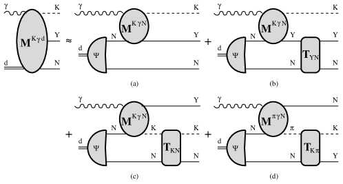
Figure 10: Kaon photoproduction on the deuteron with rescattering contributions in the two-body subsystems and the pion mediated process. Diagram (a): impulse approximation (IA); (b) and (c): $YN$ and $KN$ rescattering, respectively; (d): $\pi N\rightarrow KY$ process.

We will now describe the evaluation of each contribution in some detail.

III.1.1 The impulse approximation

In the impulse approximation the incoming photon interacts with one nucleon only producing a kaon while the other nucleon remains untouched, i.e. acts merely as a spectator. Furthermore, any subsequent interaction is neglected, thus the final state is a pure plane wave. Then the transition amplitude ${\cal M}^{K\gamma d}_{IA}$ for the diagram (a) of Fig. 10 is determined by the matrix element of the elementary kaon photoproduction operator $\widehat{\cal M}^{K\gamma N}$ taken between the deuteron bound state and the three-particle plane wave final state

$${\cal M}^{K\gamma d}_{IA,\,\mu_{Y}\mu_{N}\mu_{d}\lambda} = \langle\vec{p}_{YN}\,\vec{p}_{K}\,\mu_{Y}\,\mu_{N}|\widehat{\cal M}^{K\gamma N}|\vec{p}_{\gamma}\,\mu_{d}\,\lambda\rangle\,,$$ (60)

where the $\mu$’s denote the spin projection of the corresponding particles and $\lambda$ the photon polarization. We use for the $npd$-vertex

$$\langle\vec{p}_{N}\,\vec{p}_{N}^{\,\prime}\,1\,\mu_{S}|\vec{p}_{d}\,\mu_{d}\rangle = (2\pi)^{3}\delta^{3}(\vec{p}_{d}-\vec{p}_{N}-\vec{p}_{N}^{\,\prime})\frac{\sqrt{E_{N}E_{N}^{\prime}}}{m_{N}}\Psi_{\mu_{S}\mu_{d}}(\vec{p}\,)\,,$$ (61)

where $\vec{p}=(\vec{p}_{N}-\vec{p}_{N}^{\,\prime})/2$ denotes the relative momentum of neutron and proton in the deuteron. The deuteron wave function has the form

$$\Psi_{\mu_{S}\mu_{d}}(\vec{p}\,) = \sqrt{2E_{d}(2\pi)^{3}}\sum_{\ell=0,2}i^{\ell}C^{\ell 11}_{\mu_{\ell}\mu_{S}\mu_{d}}u_{\ell}(p)Y_{\ell\mu_{\ell}}(\hat{p})\,,$$ (62)

where $C$ denotes a Clebsch-Gordan coefficient. With $\vec{p}_{d}=0$ we obtain finally

$${\cal M}^{K\gamma d}_{IA,\,\mu_{Y}\mu_{N}\mu_{d}\lambda}(\vec{p}_{YN},\,\vec{p}_{K},\,\vec{p}_{\gamma}) = \sum_{\mu_{N^{\prime}}}{\cal M}_{\mu_{Y}\mu_{N}\lambda}^{K\gamma N}(\vec{p}_{Y},\vec{p}_{K},-\vec{p}_{N},\vec{p}_{\gamma})C^{\frac{1}{2}\frac{1}{2}1}_{\mu_{N}\mu_{N^{\prime}}\mu_{N}+\mu_{N^{\prime}}}\Psi_{\mu_{N}+\mu_{N^{\prime}}\mu_{d}}(-\vec{p}_{N})\,,$$ (63)

where $\vec{p}_{Y}=(\vec{p}_{\gamma}-\vec{p}_{K})/2+\vec{p}_{YN}$ and $\vec{p}_{N}=(\vec{p}_{\gamma}-\vec{p}_{K})/2-\vec{p}_{YN}$. This expression is straightforward to evaluate.

III.1.2 $YN$ rescattering

For the calculation of the $YN$ rescattering contribution, K. Miyagawa made available to us the routine used in YaM99 . This routine is based on the combined evaluation of the diagrams (a) and (b) of Fig. 10, i.e. the impulse approximation together with the subsequent hyperon-nucleon rescattering contribution to the photoproduction operator, which is written as

$$\widehat{\cal M}^{K\gamma d}_{IA+YN} = \widehat{\cal M}^{K\gamma d}_{IA}+\widehat{\cal M}^{K\gamma d}_{YN}$$ (64)

$$= \widehat{\cal M}^{K\gamma d}_{IA}+\widehat{\cal T}_{YN}\,\widehat{G}_{YN}\widehat{\cal M}^{K\gamma d}_{IA}\,$$ (65)

with the $YN$-scattering operator $\widehat{\cal T}_{YN}$ and $\widehat{G}_{YN}$ as the free hyperon-nucleon off-shell propagator in the presence of a non-interacting kaon. The scattering operator $\widehat{\cal T}_{YN}$ obeys the Lippmann-Schwinger equation

$$\widehat{\cal T}_{YN} = \widehat{V}_{YN}+\widehat{V}_{YN}\,\widehat{G}_{YN}\,\widehat{\cal T}_{YN}\,,$$ (66)

where $\widehat{V}_{YN}$ denotes the hyperon-nucleon potential operator introduced in Sect. II.3. Inserting Eq. (66) in Eq. (65), we get

$$\widehat{\cal M}^{K\gamma d}_{IA+YN} = \widehat{\cal M}^{K\gamma d}_{IA}+\widehat{V}_{YN}\,\widehat{G}_{YN}\widehat{\cal M}^{K\gamma d}_{IA+YN}\,,$$ (67)

which can be solved by inversion

$$\widehat{\cal M}^{K\gamma d}_{IA+YN} = \left(\widehat{1}-\widehat{V}_{YN}\,\widehat{G}_{YN}\right)^{-1}\widehat{\cal M}^{K\gamma d}_{IA}\,.$$ (68)

After solving the last equation in the partial wave decomposition with respect to the hyperon-nucleon subsystem, one obtains the $YN$ rescattering amplitude by subtraction of the impulse approximation

$${\cal M}^{K\gamma d}_{YN,\,\mu_{Y}\mu_{N}\mu_{d}\lambda}(\vec{p}_{YN},\,\vec{p}_{K},\,\vec{p}_{\gamma}) = \sum_{\ell SJ\mu_{J}}C^{\frac{1}{2}\frac{1}{2}S}_{\mu_{Y}\mu_{N}\mu_{S}}\,C^{\ell SJ}_{\mu_{\ell}\mu_{S}\mu_{J}}\,Y_{\ell\mu_{\ell}}(\hat{p}_{YN})\,$$ (69)

$$\times\left({\cal M}^{K\gamma d}_{IA+YN,\,\ell SJ,\mu_{d}\lambda}(\vec{p}_{YN},\,\vec{p}_{K},\,\vec{p}_{\gamma})-{\cal M}^{K\gamma d}_{IA,\,\ell SJ,\mu_{d}\lambda}(\vec{p}_{YN},\,\vec{p}_{K},\,\vec{p}_{\gamma})\right)\,.$$

III.1.3 $KN$ rescattering

We evaluate the $KN$ rescattering contribution (diagram (c) of Fig. 10) directly in contrast to $YN$ rescattering. The corresponding amplitude is given by

$${\cal M}^{K\gamma d}_{KN,\,\mu_{Y}\,\mu_{N}\,\mu_{d}\,\lambda}(\vec{p}_{YN},\,\vec{p}_{K},\,\vec{p}_{\gamma}) = \langle\vec{p}_{YN}\,\vec{p}_{K}\,\mu_{Y}\,\mu_{N}|\widehat{\cal T}_{KN}\widehat{G}_{KN}\widehat{\cal M}^{K\gamma N}|\vec{p}_{\gamma}\,\mu_{d}\,\lambda\rangle\,,$$ (70)

where $\widehat{\cal T}_{KN}$ is the kaon-nucleon scattering operator, $\widehat{G}_{KN}$ is the free kaon-nucleon propagator in the presence of a non-interacting hyperon. Straightforward evaluation yields

$${\cal M}^{K\gamma d}_{KN,\,\mu_{Y}\,\mu_{N}\,\mu_{d}\,\lambda}(\vec{p}_{YN},\,\vec{p}_{K},\,\vec{p}_{\gamma}) = \sum_{\mu_{N}^{\prime}}\int d^{3}p_{KN}^{\prime}\sqrt{\frac{E_{N}E_{K}}{E_{N}^{\prime}E_{K}^{\prime}}}{\cal T}_{KN,\,\mu_{N}\,\mu_{N}^{\prime}}(\vec{p}_{KN},\,\vec{p}_{KN}^{\,\prime})G_{KN}(E_{KN}-E_{KN}^{\prime})$$ (71)

$$\times\,{\cal M}^{K\gamma d}_{IA,\,\mu_{Y}\,\mu_{N}^{\prime}\,\mu_{d}\,\lambda}(\vec{p}_{YN^{\prime}},\,\vec{p}_{KN}^{\,\prime},\,\vec{p}_{\gamma})\,,$$

where $\vec{p}_{KN}$ and $\vec{p}_{KN}^{\,\prime}$ denote the relative momenta and $E_{KN}$ and $E_{KN}^{\prime}$ the total energies of the final and intermediate kaon-nucleon states, respectively, and the free propagator is given by

$$G_{KN}(z) = \frac{1}{z+i\varepsilon}=\frac{\mathcal{P}}{z}-i\pi\delta(z)\,.$$ (72)

Inserting this expression into Eq. (71), one finds as the final expression for the amplitude of the kaon-nucleon rescattering contribution

$${\cal M}^{K\gamma d}_{KN}(\vec{p}_{YN},\,\vec{p}_{K},\,\vec{p}_{\gamma}) = 2m_{KN}\sum_{\mu_{N}^{\prime}}{\mathcal{P}}\int d^{3}p_{KN}^{\prime}\sqrt{\frac{E_{N}E_{K}}{E_{N}^{\prime}E_{K}^{\prime}}}\,\frac{{\cal T}_{KN,\,\mu_{N}\,\mu_{N}^{\prime}}(\vec{p}_{KN},\,\vec{p}_{KN}^{\,\prime}){\cal M}^{K\gamma d}_{IA,\,\mu_{Y}\,\mu_{N}^{\prime}\,\mu_{d}\,\lambda}(\vec{p}_{YN^{\prime}},\,\vec{p}_{KN}^{\,\prime},\,\vec{p}_{\gamma})}{q_{KN}^{2}-(p_{KN}^{\prime})^{2}}$$ (73)

$$-i\pi\,m_{KN}\,q_{KN}\sum_{\mu_{N}^{\prime}}\int d\Omega_{KN}^{\prime}\sqrt{\frac{E_{N}E_{K}}{E_{N}^{\prime}E_{K}^{\prime}}}\,{\cal T}_{KN,\,\mu_{N}\,\mu_{N}^{\prime}}(\vec{p}_{KN},\vec{q}_{KN}^{\,\prime}){\cal M}^{K\gamma d}_{IA,\,\mu_{Y}\,\mu_{N}^{\prime}\,\mu_{d}\,\lambda}(\vec{p}_{YN^{\prime}},\,\vec{q}_{KN}^{\,\prime},\,\vec{p}_{\gamma})\,.$$

In this expression, one has $\vec{p}_{YN^{\prime}}=(\vec{p}_{Y}-\vec{p}_{N}^{\,\prime})/2$ with $\vec{p}_{N}^{\,\prime}=(\vec{p}_{\gamma}-\vec{p}_{Y}\,)/2-\vec{p}_{KN}^{\,\prime}$, and $\vec{q}_{KN}^{\,\prime}=\{q_{KN},\Omega_{KN}^{\prime}\}$ with $q_{KN}$ given by

$$q_{KN} = \sqrt{2m_{KN}\left(E_{KN}-\frac{P_{KN}^{2}}{2M_{KN}}-M_{KN}\right)}\,,$$ (74)

where $m_{KN}$ and $M_{KN}$ denote the reduced and total masses of the kaon-nucleon system, respectively.

III.1.4 $\gamma d\rightarrow\pi NN\rightarrow KYN$ process

The contribution of the diagram (d) of Fig. 10 has formally the same structure than the foregoing kaon-nucleon rescattering amplitude. We just have to replace in the final result of Eq. (73) the kaon photoproduction amplitude by the pion photoproduction amplitude and the $KN$ scattering amplitude by the $\pi N\rightarrow KY$ transition amplitude, i.e.

$${\cal M}^{K\gamma d}_{IA,\,\mu_{Y}\,\mu_{N}^{\prime}\,\mu_{d}\,\lambda}(\vec{p}_{YN^{\prime}},\,\vec{q}_{KN}^{\,\prime},\,\vec{p}_{\gamma}) \rightarrow {\cal M}^{\pi\gamma d}_{IA,\,\mu_{N}\,\mu_{N}^{\prime}\,\mu_{d}\,\lambda}(\vec{p}_{NN^{\prime}},\,\vec{q}_{\pi N}^{\,\prime},\,\vec{p}_{\gamma})\,,$$ (75)

$${\cal T}_{KN,\,\mu_{N}\,\mu_{N}^{\prime}}(\vec{p}_{KN},\,\vec{p}_{KN}^{\,\prime}) \rightarrow {\cal T}_{K\pi,\,\mu_{Y}\,\mu_{N}^{\prime}}(\vec{p}_{KN},\,\vec{p}_{\pi N}^{\,\prime})\,,$$ (76)

where ${\cal T}_{K\pi}$ and ${\cal M}^{\pi\gamma d}_{IA}$ denote the transition matrices for the pion mediated kaon process and the impulse approximation of pion photoproduction on the deuteron, respectively. The final result is

$${\cal M}^{K\gamma d}_{K\pi}(\vec{p}_{YN},\,\vec{p}_{K},\,\vec{p}_{\gamma}) = 2m_{\pi N}\sum_{\mu_{N}^{\prime}}{\mathcal{P}}\int d^{3}p_{\pi N}^{\prime}\sqrt{\frac{E_{K}E_{Y}}{E_{\pi}E_{N}^{\prime}}}\,\frac{{\cal T}_{K\pi,\,\mu_{Y}\,\mu_{N}^{\prime}}(\vec{p}_{KY},\,\vec{p}_{\pi N}^{\,\prime}){\cal M}^{\pi\gamma d}_{IA,\,\mu_{N}\,\mu_{N}^{\prime}\,\mu_{d}\,\lambda}(\vec{p}_{NN^{\prime}},\,\vec{p}_{\pi N}^{\,\prime},\,\vec{p}_{\gamma})}{q_{\pi N}^{2}-(p_{\pi N}^{\prime})^{2}}$$ (77)

$$-i\pi m_{\pi N}q_{\pi N}\sum_{\mu_{N}^{\prime}}\int d\Omega_{\pi N}^{\prime}\sqrt{\frac{E_{K}E_{Y}}{E_{\pi}E_{N}^{\prime}}}\,{\cal T}_{K\pi,\,\mu_{Y}\,\mu_{N}^{\prime}}(\vec{p}_{KY},\,\vec{q}_{\pi N}^{\,\prime}){\cal M}^{\pi\gamma d}_{IA,\,\mu_{N}\,\mu_{N}^{\prime}\,\mu_{d}\,\lambda}(\vec{p}_{NN^{\prime}},\,\vec{q}_{\pi N}^{\,\prime},\,\vec{p}_{\gamma})\,,$$

where $\vec{p}_{NN^{\prime}}=(\vec{p}_{N}-\vec{p}_{N}^{\,\prime})/2$ with $\vec{p}_{N}^{\,\prime}=(\vec{p}_{\gamma}-\vec{p}_{N}\,)/2-\vec{p}_{\pi N}^{\,\prime}$, and $\vec{q}_{\pi N}^{\,\prime}=\{q_{\pi N},d\Omega_{\pi N}^{\prime}\}$ with $q_{\pi N}$ given by

$$q_{\pi N} = \sqrt{2m_{\pi N}\left(E_{KY}-\frac{P_{\pi N}^{2}}{2M_{\pi N}}-M_{\pi N}\right)}\,.$$ (78)

Again $m_{\pi N}$ and $M_{\pi N}$ denote the reduced and total masses of the pion-nucleon system, respectively.

IV Results and discussion

The three contributions from hyperon-nucleon and kaon-nucleon rescattering and from the pion mediated process have been evaluated according to the formalism presented in Sect. III using the deuteron wave function for the Bonn OBEPQ potential of MaH87 . For the final state interaction effects we have included in $KN$ scattering partial waves up to $\ell=1$, in $YN$ scattering up to $j=1$, and in $\pi N\rightarrow KY$ only $\ell=0$.

Figure 11: Total cross sections of kaon photoproduction on the deuteron (top) and their ratios to the impulse approximation (bottom) for the separate channels $\gamma d\rightarrow K^{+}\Lambda n$ (left), $\gamma d\rightarrow K^{+}\Sigma^{0}n$ (middle), and $\gamma d\rightarrow K^{+}\Sigma^{-}p$ (right). Notation of curves: dotted: impulse approximation (IA); dash-dot: IA+YN rescattering; dashed: IA+YN+KN rescattering; solid: IA+YN+KN+$\pi N\rightarrow KY$.

We will begin with a discussion of the total cross sections for the three possible $K^{+}$-channels as shown in Fig. 11. In the upper panels we show the various effects starting with the pure impulse approximation and then adding successively $YN$ rescattering, $KN$ rescattering and finally the pion mediated contribution. In order to give a more detailed and quantitative evaluation we show in the lower panels of Fig. 11 the relative effects by plotting the ratios of the corresponding cross sections to the ones for the IA.

Figure 12: Semi-inclusive differential cross section $d\sigma/d\Omega_{K}$ for $\gamma d\rightarrow K^{+}\Lambda n$ for different photon lab energies with various interaction effects (top panels) and their ratios with respect to the impulse approximation on a logarithmic scale (bottom panels). The insets show the ratios at forward angles on a larger linear scale. Notation of curves as in Fig. 11.

Figure 13: Semi-inclusive differential cross section $d\sigma/d\Omega_{K}$ for $\gamma d\rightarrow K^{+}\Sigma^{0}n$ for different photon lab energies with various interaction effects (top panels) and their ratios with respect to the impulse approximation on a logarithmic scale (bottom panels). The insets show the ratios at forward angles on a larger linear scale. Notation of curves as in Fig. 11.

One readily notes that $KN$ rescattering – the difference between the dash-dot and the dashed curves – is quite small, almost completely negligible for the total cross section for all three channels. For $\gamma$d $\rightarrow K^{+}\Lambda n$ (left panel) one notes a sizeable enhancement near the threshold, which originates from $YN$ rescattering and the pion mediated reaction, comparable in size. At higher photon energies the enhancement is reduced to about 10 % with a slight dominance of the pion mediated process. The reaction $\gamma d\rightarrow K^{+}\Sigma^{0}n$ (middle panel) shows a different behaviour. While $YN$ rescattering decreases the cross section slightly by about $5-8$ % over the whole range of photon energies, the pion mediated contribution acts in the opposite direction leading to an overall increase compared to the IA, which is quite dramatic near threshold and is still about $20$ % at higher energies. Finally, one finds for the channel $\gamma d\rightarrow K^{+}\Sigma^{-}p$ (right panel) a significant increase by $YN$ rescattering close to threshold but above 1 GeV a small reduction of the cross section by about 5 %, a tiny increase from $KN$ rescattering, and as most dominant effect again the pion mediated process with a strong near-threshold increase which levels off above 1 GeV to about $10$ % relative to the IA. The reason for the different influence of the pion mediated reaction lies in the fact that for $K^{+}\Lambda n$ only the isospin $t=1/2$ contributes to the process $\pi N\rightarrow K\Lambda$, whereas for $\pi N\rightarrow K\Sigma$ also the more important $t=3/2$-contribution appears.

Figure 14: Semi-inclusive differential cross section $d\sigma/d\Omega_{K}$ for $\gamma d\rightarrow K^{+}\Sigma^{-}p$ for different photon lab energies with various interaction effects (top panels) and their ratios with respect to the impulse approximation on a logarithmic scale (bottom panels). The insets show the ratios at forward angles on a larger linear scale. Notation of curves as in Fig. 11.

Figure 15: Double differential cross section $d^{2}\sigma/dp_{K}d\Omega_{K}$ for $\gamma d\rightarrow K^{+}\Lambda n$ for fixed $p_{K}$ and $\theta_{K}$ as function of photon excess energies above threshold with various interaction effects. Notation of curves as in Fig. 11.

As next topic we will discuss the semi-inclusive differential cross section $d\sigma/d\Omega_{K}$ as defined in (51) for the three channels. The top panels of Fig. 12 show the differential cross sections for the channel $\gamma d\rightarrow K^{+}\Lambda n$ at three photon lab-energies, one close to the threshold, the next in the maximum of the total cross section, and finally the third above the maximum. As one notes, the kaon is produced predominantly into the forward direction, the maximum being at $0^{\circ}$ near threshold but moving to about $15^{\circ}$ at higher energies, while at backward angles the cross section drops rapidly. The reason for this behaviour is that for backward kaon production in the impulse approximation the spectator nucleon is forced to have a large momentum, for which, in turn, the deuteron wave function is strongly suppressed. In other words, the probability for finding a spectator nucleon with the appropriate momentum becomes increasingly tiny with increasing momentum transfer. In this situation it is more advantagous to share the large momentum transfer between both baryons as is provided by any of the two-step processes discussed here, particularly strong for the pion mediated process.

Figure 16: Tensor target asymmetries for channel $\gamma d\rightarrow K^{+}\Lambda n$ at different photon lab energies. Panels in the same column refer to the same photon energy. Notation of curves as in Fig. 11.

In order to see more clearly the relative size of the interaction effects we have plotted in the lower panels of Fig. 12 the ratios with respect to the IA. The insets show the ratios for forward angles on a magnified linear scale. In the forward direction $YN$ and $KN$ rescattering show at the two lower energies a small influence but opposite in sign so that the net effect is tiny. At the highest energy, one notes a sizeable increase at forward angles by $YN$ rescattering only of about 10 %. In the backward direction the situation changes completely. The aforementioned mechanism of redistributing the large momentum transfer onto two particles by two-step processes is most evident at backward angles, where one finds a huge increase of the cross section. Here $KN$ rescattering becomes more important than $YN$ rescattering, in particular at the highest energy, but most dominant is the pion mediated contribution. One also notes that the relative effect of the latter decreases with increasing energies.

Figure 17: Tensor target asymmetries for channel $\gamma d\rightarrow K^{+}\Sigma^{0}n$ at different photon lab energies. Panels in the same column refer to the same photon energy. Notation of curves as in Fig. 11.

Figure 18: Tensor target asymmetries for channel $\gamma d\rightarrow K^{+}\Sigma^{-}p$ at different photon lab energies. Panels in the same column refer to the same photon energy. Notation of curves as in Fig. 11.

The analogous results for the channel $\gamma d\rightarrow K^{+}\Sigma^{0}n$ are shown in Fig. 13. Contrary to the foregoing case, one notes for this channel in the forward direction at all photon energies a sizeable reduction from $YN$ rescattering which, however, is partially counterbalanced at the lowest energy by the $\pi\rightarrow K$ process, while $KN$ rescattering is negligible. Again the pion process becomes dominant at backward angles (see lower panels). Furthermore, $KN$ rescattering shows there a small effect like for $\gamma d\rightarrow K^{+}\Lambda n$, and $YN$ rescattering is marginal here. For the other $\Sigma$-channel, $\gamma d\rightarrow K^{+}\Sigma^{-}p$, the differential cross sections in Fig. 14 display qualitatively the same features, the reduction of the cross section in forward direction by $\Sigma N$ rescattering, which is more than compensated by the $\pi\rightarrow K$-process at the lowest energy and partially diminished at the other two energies, and a very strong enhancement at backward angles. The influence of $KN$ rescattering remains relatively small.

For a comparison with previous results of Refs. ReR67b and Ker01 we have evaluated for the channel $\gamma d\rightarrow K^{+}\Lambda n$ the double differential cross section $d^{2}\sigma/dp_{K}d\Omega_{K}$ for the same kinematics, i.e. fixed kaon momentum $p_{K}=426$ MeV and kaon angle $\theta_{K}=15^{\circ}$. The result is shown in Fig. 15 as function of the excess photon energy above threshold. The enhancement by $YN$ rescattering close to threshold is very similar to ReR67b ; Ker01 . In this energy region the $\pi\rightarrow K$ process shows little effect. However, above the peak this process becomes increasingly more important as one readily notes in Fig. 15. A comparison to the work of Maxwell Max04 is not possible since in Max04 total and semi-inclusive cross sections were not given.

As last topic, we will discuss the influence of interaction effects on polarization observables for which we have chosen the tensor target asymmetries for a tensor polarized deuteron target. Fig. 16 shows the three types of asymmetries $T_{20}$ (top panels), $T_{21}$ (middle panels), and $T_{22}$ (bottom panels) for the channel $\gamma d\rightarrow K^{+}\Lambda n$ at the same photon lab energies as for the differential cross sections. As can be seen in the top panels of Fig. 16, the tensor target asymmetry $T_{20}$ is relatively small at forward angles for all given photon energies, and interaction effects show little influence, while at backward angles they become much more pronounced. Their effect changes quite strongly with energy. At the lowest energy $YN$ rescattering shows little influence whereas $KN$ rescattering changes $T_{20}$ from $-1$ for IA to 0.4 which is then reduced to $-0.2$ by the pion process. At $E_{\gamma}=1.14$ GeV $YN$ rescattering reduces $T_{20}$ at 180^∘ from $-0.2$ for IA to almost zero, then it is increased to 0.13 by $KN$ rescattering to be reduced again to $-0.12$ by the pion contribution. For the highest energy $T_{20}$ is changed from $-0.01$ for IA to 0.07 by all interaction effects.

For $T_{21}$ and $T_{22}$ in the middle and bottom panels of Fig. 16, respectively, one also notes quite a variation with the various interaction contributions, their relative influence varying quite strongly with photon energy. The $\pi\rightarrow K$ process counteracts in general the influence of $YN$ and $KN$ rescattering. The final results for $T_{21}$ show a positive forward peak with a size between 0.2 at the lowest energy and 0.03 at the highest one, and a negative minimum around 90^∘ of $-0.1$ to $-0.03$. $T_{22}$ develops a negative minimum around 100-110^∘ of the order of 0.06-0.03 for the highest two energies.

The tensor target asymmetries for channel $\gamma d\rightarrow K^{+}\Sigma^{0}n$ are shown in Fig. 17. The top panels of this figure show that the values of $T_{20}$ are again relatively small in the forward region. The various rescattering contributions add constructively so that at backward angles the negative values for $T_{20}$ in IA is changed to positive values of 0.3 to 0.18 going from the lowest to the highest energy. At the highest energy, $YN$ rescattering has quite a small effect as shown in the right top panel of Fig. 17. In the middle panels one can see that $KN$ rescattering has quite a strong effect on $T_{21}$ at the lowest energy but becomes small for the two higher energies where the two-step process results in a positive maximum of about 0.04. Remarkable influence of $KN$ rescattering is seen in $T_{22}$ in the bottom panels of Fig. 17. But the two-step process counteracts again so that altogether quite a small size of the order 0.005 results.

Finally, Fig. 18 exhibits the tensor target asymmetries for the reaction $\gamma d\rightarrow K^{+}\Sigma^{-}p$. For the asymmetry $T_{20}$ one readily notes a sizeable influence from $YN$ rescattering while $KN$ rescattering shows a strong effect only for the lowest energy. Again the pion process acts in the opposite direction resulting in a total value of 0.2 to 0.1 at backward angles. In $T_{21}$ $KN$ rescattering exhibits a remarkable influence which, however, is compensated by the pion contribution. A similar situation is found for $T_{22}$. The total result shows a small forward positive peak and a negative minimum at higher angles of the order $-0.01$.

V Summary and conclusions

Kaon photoproduction on the deuteron has been investigated with respect to the importance of final state interactions, i.e. $YN$ and $KN$ rescattering, and of a two-body photoproduction contribution in terms of a pion mediated process $\gamma d\rightarrow\pi NN\rightarrow KYN$. The latter turned out to give the dominant contribution beyond the IA, except for $\gamma d\rightarrow K^{+}\Lambda n$ near threshold where the influence of $\Lambda N$ rescattering is comparable to the pion process. The latter leads to an increase of the total cross section relative to the IA. The increase is particularly large in the near threshold region for the $K\Sigma$ channels. This effect has its origin in the considerably stronger pion photoproduction amplitude on the nucleon compared to the corresponding amplitude for the kaon photoproduction in combination with a sizeable $\pi N\rightarrow KY$ strangeness exchange reaction. Next in importance is $YN$ rescattering while $KN$ rescattering is much smaller. The overall enhancement of the total cross section from all interaction effects is about 2 % at the peak for $\gamma d\rightarrow K^{+}\Lambda n$, 10 % for $\gamma d\rightarrow K^{+}\Sigma^{0}n$, and 7 % for $\gamma d\rightarrow K^{+}\Sigma^{-}p$.

The semi-inclusive differential cross sections show that the kaon is mostly produced in the forward direction where the impulse approximation works reasonably well. But for a precise description, at least the effects from YN rescattering and the $\pi\rightarrow K$-process have to be considered. At backward angle, the strongest enhancement arises from the pion mediated process. As expected on general grounds, the tensor target asymmetries $T_{20}$, $T_{21}$, and $T_{22}$ exhibit a much stronger sensitivity to the various interaction effects, in particular at backward angles.

Therefore, we may state as general conclusion that for studying the elementary kaon photoproduction on the neutron in the reaction on the deuteron the influence of interaction effects have to be cleanly separated using a reliable theoretical model. The same caveat applies for the study of the hyperon-nucleon interaction in this reaction.

At present such interaction effects are treated in an approximate way by including them completely only in the two-body subsystems. Thus an extension to a three-body formalism is desirable for the future in kinematic regions where such interaction effects appear substantial. Furthermore, instead of the simple separable potentials used in the present work, more realistic potentials for $KN$ scattering and the $\pi\rightarrow K$ process should be considered. Also the model for the electromgnetic production operator could be improved, in particular the question of gauge invariance should be addressed more carefully. Moreover, the present formalism can also be extended to study kaon electroproduction on the deuteron in order to exploit the additional degrees of freedom of virtual photons.

References

• (1) H. Thom, Phys. Rev. 151, 1322 (1966).
• (2) R.A. Adelseck, C. Bennhold, and L.E. Wright, Phys. Rev. C 32, 1681 (1985).
• (3) J.C. David, C. Fayard, G.H. Lamot, and B. Saghai, Phys. Rev. C 53, 2613 (1996).
• (4) T. Mart, Dissertation, Johannes Gutenberg UniversitΓ€t, Mainz, 1996.
• (5) C. Bennhold, T. Mart, and D. Kusno, Proc. of The CEBAF/INT Workshop on $N^{\ast}$ Physics, Seattle USA, 1996.
• (6) T. Mart, Phys. Rev. C 62, 038201 (2000).
• (7) F.X. Lee, T. Mart, C. Bennhold, H. Haberzettl, and L.E. Wright, Nucl. Phys. A695, 237 (2001).
• (8) H. Haberzettl, C. Bennhold, T. Mart, and T. Feuster, Phys. Rev C 58, R40 (1998).
• (9) B.S. Han, M.K. Cheoun, K.S. Kim, and I.T. Cheon, Nucl. Phys. A691, 713 (2001).
• (10) S. Janssen, J. Ryckebusch, D. Debruyne, and T.V. Cauteren, Phys. Rev. C 65, 015201 (2002).
• (11) M. Bockhorst et al., Z. Phys. C 63, 37 (1994).
• (12) M.Q. Tran et al., Phys. Lett. B445, 20 (1998).
• (13) X. Li, L.E. Wright, and C. Bennhold, Phys. Rev. C 45, 2011 (1992).
• (14) F.M. Renard and Y. Renard, Nucl. Phys. B1, 389 (1967).
• (15) F.M. Renard and Y. Renard, Phys. Lett. B24, 159 (1967).
• (16) R.A. Adelseck and L.E. Wright, Phys. Rev. C 39, 580 (1989).
• (17) H. Yamamura, K. Miyagawa, T. Mart, C. Bennhold, H. Haberzettl, and W. GlΓΆckle, Phys. Rev. C 61, 014001 (1999).
• (18) P.M.M. Maessen, Th.A. Rijken, and J.J. de Swart, Phys. Rev. C 40, 2226 (1989).
• (19) Th.A. Rijken, V.G.J. Stoks, and Y. Yamamoto, Phys. Rev. C 59, 21 (1999).
• (20) B.O. Kerbikov, Phys. Atom. Nucl. 64, 1835 (2001).
• (21) O.V. Maxwell, Phys. Rev. C 69, 034605 (2004).
• (22) J.D. Bjorken and S.D. Drell, Relativistic Quantum Mechanics, Mc Graw-Hill Inc., New York, 1964.
• (23) A. Donnachie, High Energy Physics, Vol. 5, Academic Press, New York, 1972.
• (24) A. Salam, Dissertation, Johannes Gutenberg UniversitΓ€t, Mainz, 2003.
• (25) S. Goers et al., Phys. Lett. B464, 331 (1999).
• (26) D. Drechsel, O. Hanstein, S.S. Kamalov, and L. Tiator, Nucl. Phys. A645, 145 (1999).
• (27) G.F. Chew, M.L. Goldberger, F.E. Low, and Y. Nambu, Phys. Rev. 106, 359 (1957).
• (28) J.S. Hyslop, R.A. Arndt, L.D. Roper, and R.L. Workman, Phys. Rev. D 46, 961 (1992).
• (29) W. Cameron et al., Nucl. Phys. B78, 93 (1974).
• (30) K. Abe et al., Phys. Rev. D 11, 1719 (1975).
• (31) T.M. Knasel et al., Phys. Rev. D 11, 1 (1975).
• (32) D.H. Saxon et al., Nucl. Phys. B162, 522 (1980).
• (33) D.J. Candlin et al., Nucl. Phys. B226, 1 (1983).
• (34) R.D. Baker et al., Nucl. Phys. B145, 402 (1978).
• (35) J.C. Hart et al., Nucl. Phys. B166, 73 (1979).
• (36) M.L. Good et al., Phys.Rev. 183, 1142 (1969).
• (37) O.I. Dahl et al., Phys. Rev. 163, 1430 (1967).
• (38) H. ArenhΓΆvel, Few-Body Syst. 4, 55 (1988).
• (39) A.R. Edmonds, Angular Momentum in Quantum Mechanics, Princeton Univ. Press, Princeton, 1957.
• (40) R. Machleidt, K. Holinde, and Ch. Elster, Phys. Rep. 149, 1 (1987).