Order parameter fluctuations in percolation: Application to nuclear multifragmentation

Abstract

Order parameter fluctuations (the largest cluster size distribution) are studied within a three-dimensional bond percolation model on small lattices. Cumulant ratios measuring the fluctuations exhibit distinct features near the percolation transition (pseudocritical point), providing a method for its identification. The location of the critical point in the continuous limit can be estimated without variation of the system size. This method is remarkably insensitive to finite-size effects and may be applied even for a very small system. The possibility of using various measurable quantities for sorting events makes the procedure useful in studying clusterization phenomena, in particular nuclear multifragmentation. Finite-size scaling and $\Delta$-scaling relations are examined. The model shows inconsistency with some of the $\Delta$-scaling expectations. The role of surface effects is evaluated by comparing results for free and periodic boundary conditions.

I Introduction

The main motivation of nuclear multifragmentation studies is probing a liquid-gas coexistence region in the phase diagram of nuclear matter Siemens ; Jaq ; good . Many works deduce the occurrence of a first- or second-order phase transition Finn ; gil ; poch ; ago ; d-p ; gupta ; kleine ; fis ; nat ; sri ; ma . Although both transition types can be expected, unambiguous identification is difficult due to strong finite-size effects in systems with a small number of constituents. In such systems, for example, a first-order phase transition may mimic critical behavior mim ; car . On the other hand, nuclear multifragmentation induced by high energy collisions shows striking similarities to percolation processes which are known to contain a second-order phase transition (critical behavior) kleine ; b1 ; b2 ; c1 ; c2 ; kreutz ; li ; hyp . Percolation-based models seem to be also successful in describing fragmentation of atomic clusters far ; gobet . These observations lead to formulation of the hypothesis that percolation could be a universal fragmentation mechanism for simple fluids hyp . For better recognizing critical-like behavior observed in fragmentation processes, simultaneous application of various complementary methods is necessary. Percolation models are often used to construct or verify procedures tracing critical behavior in fragmenting systems b1 ; b2 ; c1 ; c2 ; el ; ell ; d-e ; uf . They provide a simple tool for studying universal aspects of the critical behavior and the role of finite-size effects.

In the framework of a percolation model we have examined the largest cluster size distribution. The size of the largest cluster, as an order parameter in aggregation scenarios of the fragment production, is of particular interest in phase transition studies d-e ; uf . The limiting forms of the distribution for normal phases are predicted by classical limit theorems for random variables uf ; d-n ; baz1 ; baz2 . At a second-order phase transition the system is highly correlated with fluctuations occurring on all length scales. Properties of the order parameter close to the critical point can be studied with the renormalization group and finite-size scaling approaches d-e ; uf ; d-n ; baz2 ; sta ; binder . Botet and Płoszajczak have proposed to identify the second-order critical behavior in finite systems by examining universal features of the order parameter fluctuations with a $\Delta$-scaling method d-p ; d-e ; uf ; d-n . The method has been applied to several models and nuclear fragmentation data d-p ; ma ; car ; d-e ; uf ; fra ; frank ; frankland ; gul . We will confront $\Delta$-scaling predictions with percolation results.

In order to compare theoretical predictions with fragmentation data all experimental conditions should be carefully considered. The bulk behavior of the order parameter can be significantly modified in small fragmenting systems by finite-size and boundary effects. The control parameter is usually not well measured and must be substituted by other measurable quantities in sorting events, leading to additional modifications. We aim to evaluate the significance of such effects in the present work.

The calculations were performed with a three-dimensional bond percolation model on the simple cubic lattices sta . A Monte Carlo procedure with the Hoshen-Kopelman cluster labeling algorithm was employed to generate events for a distribution of the bond probability, $p$, being the control parameter. The lattices of size $N=L^{3}$ with $L=3,4,5,6$ correspond to the range of system sizes available in nuclear reactions. Free boundary conditions were applied to account for the presence of surface in real systems. To evaluate the role and importance of finite-size and boundary effects the calculations were extended to include larger systems and periodic boundary conditions.

We study low-order cumulants (cumulant ratios) as the mean, variance, skewness and kurtosis of the largest cluster size distribution. These standard statistical measures contain the most significant information, providing a robust identification of the percolation transition. In order to place our results in a wider context, we will briefly recall in the next section some signals of criticality that are frequently tested in fragmentation studies.

II Percolation transition in small systems

In the strictest sense, the phase transition occurs in the continuous limit $N\rightarrow\infty$. Then, below the percolation threshold $p<p_{c}\simeq 0.2488$, only finite clusters are present. When $p>p_{c}$ there exists an infinite cluster spanning the whole lattice. The fraction of sites belonging to this cluster is the order parameter. In finite systems the transition is smoothed. The probability that at least one cluster connects the bottom and the top lattice planes changes gradually as illustrated in Fig. 1(a).

Figure 1: Bond percolation on a lattice of linear size $L=5$ with free boundary conditions. Plotted as a function of the bond probability: (a) the probability that a lattice is spanned, (b) moments of the average distribution of cluster sizes, (c) the variance of the largest cluster size distribution with various normalizations. (d) The average distribution of cluster sizes.

A natural way to locate the transition is to examine quantities which diverge at the critical point in the continuous limit. For finite systems, the divergence is replaced by a maximum located near $p_{c}$. This can be seen in Fig. 1(b) for the second moment of the average distribution of cluster sizes, $M_{2}$, the mean cluster size, $M_{2}/M_{1}$, and the reduced variance, $\gamma_{2}\equiv M_{2}M_{0}/M_{1}^{2}$ c2 . $M_{k}$ denotes the $k$-th moment of the cluster size distribution, $M_{k}=\sum_{s}s^{k}n_{s}$, where $n_{s}$ is the average number of clusters of size $s$ normalized to the system size (the largest cluster excluded). The mean cluster size is the analog of the susceptibility and the location of its maximum value defines the pseudocritical point. Another frequently used method is a power-law fit to the fragment size distribution Finn ; ell . In our example the best fit is obtained for $p=0.33$ as shown in Fig. 1(d). The fragment size distribution follows in some range the asymptotic behavior $n_{s}=q_{0}s^{-\tau}$, where the Fisher exponent $\tau=2.189$ exp . The normalization constant $q_{0}=1/\sum_{s=1}^{\infty}s^{(1-\tau)}$ is taken as $0.173$ from the summation computed up to $s=10^{9}$. Another example is the maximum fluctuation of the largest cluster size. The size of the largest cluster, $s_{max}$, plays the role of an extensive order parameter. Its fluctuations are usually measured by the variance, $\kappa_{2}$, or the normalized variance, $\kappa_{2}/\langle s_{max}\rangle$, of the probability distribution $P(s_{max})$ c2 ; ell ; hyp ; dorso . The two quantities are peaked in the transition region as shown in Fig. 1(c) by the dotted and dashed lines. When using the normalization $\kappa_{2}/\langle s_{max}\rangle^{2}$, the maximum is located remarkably close to the critical point.

The above examples show that various investigated signals appear at different positions and in most cases they are shifted from the critical point toward the ordered phase region. In small systems the shifts may be significant and should be taken into account in a criticality analysis. The location of the critical region in nuclear multifragmentation is often deduced from a power-law fit to the fragment size distribution. This location, appearing near the pseudocritical point, would correspond to a temperature $T_{pc}$ distinctly lower than the true critical temperature $T_{c}$. For example, converting the bond probability to the temperature with the prescription of Ref. li ; babo , one obtains $T_{pc}/T_{c}=0.64,0.73$ and 0.78 for $N=27,64$ and 125, respectively.

The location of the true critical point, $p_{c}$, is of particular interest. According to the finite-size scaling the position of a signal, $p(L)$, is expected to converge to $p_{c}$ with increasing linear lattice size $L$ as

$$p(L)-p_{c}\propto L^{-1/\nu},$$ (1)

where $\nu$ is the correlation length exponent. Estimation of a critical point by such an extrapolation method seems to be difficult in the case of nuclear multifragmentation. Sizes of fragmenting systems created in nuclear reactions are not well controlled due to the preequilibrium emission and their range is limited. In addition, one may expect large departures from the scaling relation of Eq. (1) for very small systems. Our observation is that, without relying on the finite-size scaling, the best estimation of the critical point is given by the position of the maximum of $\kappa_{2}/\langle s_{max}\rangle^{2}$. Behavior of this quantity for different system sizes and various event sortings will be investigated in the following sections.

III Order parameter fluctuations

III.1 Cumulants and finite-size scaling

The order parameter probability distribution representative for small lattices with open boundaries is shown in Fig. 2 for various values of $p$. Far from the transition the distribution is sharply peaked with an extended tail to the right (left) in the disordered (ordered) phase and positioned close to the limiting values. In the transition region the distribution rapidly evolves passing through a broad, flattened and (nearly) symmetrical distribution. This behavior can be well characterized by using the skewness, $K_{3}$, measuring the asymmetry of a distribution and the kurtosis excess, $K_{4}$, which quantifies the degree of peakedness.

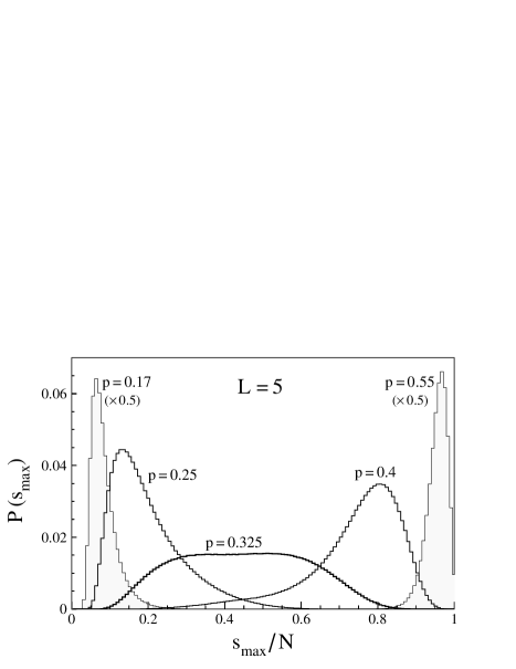
Figure 2: Probability distributions of the largest cluster size for a lattice of size $N=125$ with free boundary conditions.

The quantities of interest are defined and expressed in terms of the cumulants as

$$K_{2}\equiv \mu_{2}/\langle s_{max}\rangle^{2} =\kappa_{2}/\kappa_{1}^{2}$$

$$K_{3}\equiv \mu_{3}/\mu_{2}^{3/2} =\kappa_{3}/\kappa_{2}^{3/2}$$

$$K_{4}\equiv \mu_{4}/\mu_{2}^{2}-3 =\kappa_{4}/\kappa_{2}^{2},$$ (2)

where $\mu_{i}=\langle(s_{max}-\langle s_{max}\rangle)^{i}\rangle$ is the $i$-th central moment, and $\kappa_{i}$ is the $i$-th cumulant of the $P(s_{max})$ distribution. They are plotted as a function of $p$ for different system sizes in Fig. 3(a). In the vicinity of the critical point and for $L\rightarrow\infty$ one expects for these dimensionless parameters the scaling relation

$$K_{i}=f_{i}[(p-p_{c})L^{1/\nu}].$$ (3)

If the scaling holds, values of $K_{i}$ at $p_{c}$ are independent of the system size, which is approximately observed in our plots as the crossing of curves for different $L$ near $p_{c}$.

Figure 3: The cumulant ratios of Eq. (2) as a function of the bond probability (a) and the scaling variable (b) for systems of different sizes. Calculations with free boundary conditions.

To verify the scaling in the neighborhood of the critical point the $K_{i}$ parameters are replotted in Fig. 3(b) against the scaling variable $(p-p_{c})L^{1/\nu}$, where $\nu=7/8$. The collapse of the data shows that the scaling relation with no corrections for finite-size effects is well satisfied even for such small lattices with open boundaries. As can be estimated from Fig. 3(b) the asymptotic values of $K_{i}$ at $p_{c}$ are about $K_{2}=0.24$, $K_{3}=1.2$, and $K_{4}=1.5$. For small systems they are somewhat smaller with largest deviations observed for $K_{2}$. A prominent feature of the $K_{2}$ distribution is the maximum located very close to $p_{c}$ irrespective of the system size.

Another characteristic point, corresponding to the broad transitional distribution shown in Fig. 2, is where $K_{3}=0$ and $K_{4}$ reaches its minimum value of about $-0.9$, and $K_{2}\simeq 0.135$. It is observed at some distance from the critical point, which depends on the system size as $(p-p_{c})\simeq 0.5L^{-1/\nu}$. This point approximately coincides with the maximum of the mean cluster size and the power-law behavior of the fragment size distribution (see Fig. 4), and may be used as an estimation of the pseudocritical point. The line in Fig. 4 is a power-law fit of Eq. (1) to such points giving $\nu=0.878\pm 0.005$ in agreement with the expected value $\nu=0.875$. Corrections to the scaling are not significant in this case. Other variables considered in Fig. 4 show much larger deviations from the asymptotic scaling behavior.

The above characteristics are for free boundary conditions. Behavior of $K_{i}$ for periodic boundary conditions when surface effects are reduced is shown in Fig. 5. Also in this case the finite-size scaling features are clearly observed. As expected, the scaling functions $f_{i}$ are compressed now toward lower bond probabilities, which can be seen by comparing Fig. 5(b) with Fig. 3(b). The pseudocritical point is positioned very close to the critical point. Thus, the large difference in locations of these points in the case of free boundary conditions may be interpreted as a surface effect.

Figure 4: Finite-size scaling plot for values of the bond probability, $p$, at which the conditions indicated on the figure are fulfilled. The line is the best linear fit to the open circles.

Figure 5: Same as Fig. 3 for periodic boundary conditions. The dots in the left part indicate the $K_{3}$ and $K_{4}$ values for the Gumbel distribution (see text).

Figure 6: The normalized variance of $P(s_{max})$ versus the bond probability for free boundary conditions (a), and periodic boundary conditions (b).

III.2 Delta scaling

Behavior of the cumulant moments is of interest in the context of $\Delta$-scaling proposed for studying criticality in finite systems d-p ; d-e ; uf ; d-n . Probability distributions $P(s_{max})$ of the extensive order parameter, $s_{max}$, for different “system sizes”, $\langle s_{max}\rangle$, obey $\Delta$-scaling if they can be converted to a single scaling function $\Phi(z_{(\Delta)})$ by the transformation

$$\langle s_{max}\rangle^{\Delta}P(s_{max})=\Phi(z_{(\Delta)})\equiv\Phi\left(\frac{s_{max}-\langle s_{max}\rangle}{\langle s_{max}\rangle^{\Delta}}\right),$$ (4)

where $1/2\leq\Delta\leq 1$. It was argued that the order parameter satisfies the “first-scaling law” ($\Delta=1$ scaling) for systems at the critical point and in the disordered phase. The “second-scaling law” ($\Delta=1/2$) applies for systems in the ordered phase far from the transition point. Using a three-dimensional bond percolation model, it was demonstrated that the $\Delta=1$ scaling holds near the critical point while the $\Delta=1/2$ scaling is satisfied above the percolation threshold at $p=0.35$ d-e ; uf . However, these results were obtained for rather large systems $N=14^{3}$ to $32^{3}$ with periodic boundary conditions. In the following, we examine the scaling properties in a wide range of the control parameter, also for smaller systems with open boundaries.

In case of a $\Delta$-scaling the normalized cumulants $\kappa_{i}/\kappa_{1}^{i\Delta}$ are independent of the “system size”, $\kappa_{1}\equiv\langle s_{max}\rangle$. Therefore, for a set of $P(s_{max})$ distributions, $K_{3}=\mathrm{const}$ and $K_{4}=\mathrm{const}$ are necessary conditions for a $\Delta$-scaling. Additionally, $K_{2}=\mathrm{const}$ for $\Delta=1$, and $\kappa_{2}/\kappa_{1}=\mathrm{const}$ for $\Delta=1/2$. The conditions for the $\Delta=1$ scaling are fulfilled only in the vicinity of the critical point. The crossing points seen in Figs. 3(a) and 5(a) indicate the system size independence of $K_{i}$ near $p_{c}$. The conditions are also satisfied around the critical point when both the system size and the control parameter are varied so that $(p-p_{c})L^{1/\nu}=\mathrm{const}$, accordingly to the finite-size scaling. Since the conditions are necessary but not sufficient, we have checked that indeed the scaling relation of Eq. (4) is approximately satisfied. Observing the $\Delta=1$ scaling requires then a variation of the system size without or with a very specific change of the control parameter. It cannot be observed when the system size is fixed. A similar conclusion has been reached in Ref. gul for a lattice gas model. This contradicts the statement of Refs. d-e ; uf ; d-n that the scaling relation is valid independently of any phenomenological reasons for changing the “system size”.

Fig. 5(a) shows no evidence for the presence of a $\Delta$-scaling in the subcritical region $p<p_{c}$ (disordered phase). The largest cluster size in subcritical percolation have been extensively studied in Ref. baz1 . As predicted by the theory of extremes of independent random variables, $P(s_{max})$ converges to the Fisher-Tippett (Gumbel) distribution when $N\rightarrow\infty$. The mean grows logarithmically with the system size while the variance is bounded. Such a behavior cannot be described by a $\Delta$-scaling. For the Gumbel distribution $K_{3}\simeq 1.14$ and $K_{4}=2.4$, marked in Fig. 5(a) by the dots. As can be seen, the small systems show significant deviations from these asymptotic values even for periodic boundary conditions.

The limiting behavior of the largest cluster size in the supercritical region $p>p_{c}$ (ordered phase) is governed by the Central Limit Theorem uf ; baz2 . The asymptotic distribution is Gaussian, $K_{3}=K_{4}=0$, with the mean and variance both increasing linearly with the system size, $\kappa_{2}/\kappa_{1}=\mathrm{const}$, satisfying the $\Delta=1/2$ scaling relation. Such characteristics are seen in Figs. 5(a) and 6(b) away from the critical point for larger systems with periodic boundary conditions. Since the normalized variance $\kappa_{2}/\kappa_{1}$, same for all $N$, systematically decreases with $p$, the scaling can only be observed for fixed $p$ and different $N$. Considering very small systems $L=3$ to 6 with free boundary conditions as appropriate for nuclear applications, Fig. 6(a) shows that $\kappa_{2}/\kappa_{1}$ at fixed $p$ strongly depends on the system size. This indicates the violation of the scaling as a consequence of surface effects.

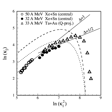
Figure 7: Log-log plot of the variance versus the squared mean value of the largest fragment size (charge) distribution. The points are experimental data for events sorted according to the excitation energy fra . The lines are percolation results for $N=64$ when events are sorted by the bond probability (dashed line) and by the fraction of open bonds (dotted line).

Figure 8: Percolation lattice of 64 sites with open boundaries. (a) The normalized variance of $P(s_{max})$ as a function of the bond probability. (b) The variance versus the squared mean in log-log representation for events binned by $p$.

Investigations of the largest fragment charge distribution, $P(Z_{max})$, observed in heavy-ion central collisions at bombarding energies between 25 and 150 $A$MeV have shown that $\kappa_{2}/\kappa_{1}\simeq\mathrm{const}$ at lower energies while $K_{2}\simeq\mathrm{const}$ in a high energy range d-p ; fra ; frank . The two regimes appear on the $\ln(\kappa_{2})$ versus $\ln(\kappa_{1}^{2})$ plot along two lines with the slope of $1/2$ and 1. This observation has been interpreted as the presence of the two limiting $\Delta$-scaling laws corresponding to the ordered and disordered phases (in the case of $\Delta$-scaling the slope is equal to $\Delta$). Fig. 7 shows such a plot when experimental events are sorted according to the estimated source excitation energy. These data taken from Ref. fra include quasi-projectiles from Ta + Au collisions allowing to observe a strong suppression of the fluctuations at lowest energies. Assuming the percolation pattern of the cumulants, interpretation of the high energy branch in terms of the $\Delta=1$ scaling would require that for different excitation energies all fragmenting systems are created with nearly the same value of a control parameter close to a critical point. More realistically, the control parameter varies with the excitation energy while changes of the system size are less significant. The dashed and dotted lines in Fig. 7 show percolation results for fixed $N=64$ when events are binned by the bond probability and by the fraction of open bonds. Given the mean, the variance depends not only on the system size but also on the choice of binning variable. For a quantitative comparison with the data one would have to determine appropriate system sizes and a sorting variable equivalent to the excitation energy. Nevertheless, the qualitative behavior of the lines shows similarity to the experimental data. The model suggests that the slope changes continuously and, as is shown in Fig. 8, the point with slope of 1 corresponds to the maximum of $K_{2}$ (locally $K_{2}\simeq\mathrm{const}$), whereas the slope of $1/2$ reflects the maximum of $\kappa_{2}/\kappa_{1}$. These features are not related to a $\Delta$-scaling. The rise and fall behavior of the correlation in Fig. 7 is a simple consequence of the mass conservation constraint. Some points on this line may have a particular meaning depending on the assumed model. In the present model, the point of slope 1 approximately corresponds to the critical point. Within the canonical lattice gas model the point of maximum variance occurs close to the critical point at the critical density. For subcritical densities it is located inside the coexistence region gul .

III.3 Event sorting effects

The cumulant properties of the largest cluster size distribution presented above are for an ideal situation, which assumes that generated events are sorted according to precisely known values of the control parameter. In experimental studies such a selection is difficult to realize. Usually the sorting parameter is a measurable quantity (e.g., multiplicity, excitation energy per nucleon) which is correlated with the control parameter with a significant dispersion.

Figure 9: The cumulant ratios as a function of the fraction of open bonds; on top the correspondence to the mean value of the bond probability.

Even if an attempt is made to estimate a control parameter such as the temperature in nuclear multifragmentation, some dispersion is unavoidable. This can be simulated by using the fraction of open bonds, $q$, for sorting events. On average, the relation between $p$ and $q$ is linear, $q\simeq 1-p$, for all system sizes. Fig. 9 presents $K_{i}$ as a function of $q$ for small lattices of $L=3$ to $6$ with open boundaries which are relevant for nuclear multifragmentation studies. The top diagram shows the correspondence between $q$ and $\langle p\rangle$. Comparing $K_{i}(q)$ with $K_{i}(p)$ in corresponding intervals shows that absolute values may change significantly, however, some characteristic features are approximately preserved. The $K_{2}(q)$ distributions exhibit maxima near the “critical” value $q_{c}\simeq 0.75$ corresponding to $p_{c}$. The zeros of $K_{3}(q)$ coincide with the minima of $K_{4}(q)$ reflecting the behavior near the pseudocritical point. However, at the “critical” point, $q_{c}$, the cumulant values are now much smaller and differ with the lattice size. The crossing points appear shifted from $q_{c}$ toward the ordered phase. These intersection points are spread out over some range of $q$ and are expected to converge to $q_{c}$ with increasing $N$. The relation between $p$ and the number of broken bonds is governed by a binomial distribution. This implies that for a given $q$, the dispersion of $p$ vanishes as $\sim N^{-1/2}$ with $N\rightarrow\infty$. On the other hand, according to the finite-size scaling, $K_{i}(p)$ follows the same pattern irrespective of $N$ within a fixed interval of the scaling variable $(p-p_{c})L^{1/\nu}$. Thus, the corresponding interval of $p$ vanishes with increasing $N$ as $\sim N^{-1/3\nu}\simeq N^{-1/2.625}$. Since the dispersion vanishes faster, the limiting distributions $K_{i}(q)$ and $K_{i}(p)$ will be equivalent: $K_{i}(q)\rightarrow K_{i}(p=1-q)$ when $N\rightarrow\infty$. Significant differences between the sortings are observed in small systems.

Figure 10: The cumulant ratios as a function of the normalized multiplicity.

Figure 11: The cumulant ratios as a function of the normalized total size of complex fragments.

Figure 12: Parameters of the “critical” point as a function of the system size when events are binned according to the multiplicity (left column) and $S_{bound}$ (right column). The points show percolation values, the lines represent approximations by Eq. (5).

Particularly interesting is sorting events according to directly measurable quantities. We have examined the $K_{i}$ dependencies on the overall multiplicity, $m$, (Fig. 10) and the total size of all clusters of size greater than $1$, $S_{bound}$, (Fig. 11). The parameters are normalized to the system size $N$. In both cases the average correspondence to the control parameter depends on the system size, which is shown in the top diagrams where the solid line is for $L=6$ and the dotted one for $L=3$. The $K_{2}$ distributions exhibit maxima whose positions correspond to the critical value of the control parameter, $p_{c}$. For such “near-critical” events, values of the sorting variables and the cumulant ratios depend on the system size as shown in Fig. 12. They all can be well described by the equation

$$X=a-\frac{c}{N+b},$$ (5)

with coefficients $a,b$, and $c$ listed in Table I. In practice, when the system size in not well known, one can examine $K_{i}$ as a function of $m$ (and/or $S_{bound}$). The system size $N$ can be found by solving Eq. 5 with $X=m/N$ for $m=m_{c}$ at which the maximum of $K_{2}$ is observed. Then, the values of $K_{2},K_{3},$ and $K_{4}$ calculated from Eq. 5 can be verified with those observed at $m=m_{c}$.

For all the considered sortings, $K_{3}=0$ occurs at the same position as the minimum of $K_{4}$, near the maximum of the mean cluster size and a point where the best power-law fit to the fragment size distribution is observed. Therefore, such a point may be used as an alternative or complementary indication of the pseudocritical point. The minimum value of $K_{4}$ is close to $-1$ for all the sorting parameters and system sizes.

Figs. 10 and 11 show that the crossing points, as it was for the sorting by $q$, are shifted from the “critical” point corresponding to $p_{c}$ toward the ordered phase region. For $S_{bound}/N$ they are well localized near the pseudocritical point. In this case the pseudocritical point can be additionally characterized by $K_{2}\simeq 0.15$ and the position $S_{bound}/N\simeq 0.84$.

In our simulations events have been generated for uniformly distributed values of the bond probability, $p$, and then grouped in bins of a sorting variable. Using a different distribution of $p$ changes the spectrum of events in a bin. Consequently, quantities such as $K_{i}$ calculated for events within a bin may also change their values. Calculations performed for a gaussian distribution of $p$ which might simulate experimental conditions have shown that this effect is of minor importance.

Table 1: The coefficients of Eq. (5) for events grouped in bins of the multiplicity (upper part) and $S_{bound}$ (lower part).

X	$a$	$b$	$c$
$m/N$	$0.352$	$28.$	$-9.6$
$K_{2}$	$0.187$	$44.$	$6.8$
$K_{3}$	$1.03$	$19.$	$15.$
$K_{4}$	$0.91$	$26.$	$47.$
$S_{bound}/N$	$0.777$	$23.$	$6.$
$K_{2}$	$0.27$	$7.$	$2.6$
$K_{3}$	$1.27$	$8.$	$10.$
$K_{4}$	$1.74$	$16.$	$53.$

IV Conclusions

The largest cluster size distributions have been examined within a percolation model on small lattices with open boundaries. The dimensionless cumulant ratios as the normalized variance, $K_{2}$, the skewness, $K_{3}$, and the kurtosis, $K_{4}$, of the distribution satisfy with a good accuracy the finite-size scaling in the critical region. In particular, $K_{i}$ are independent of the system size near the critical point (crossing points). This feature has been explored in phase transition studies as the cumulant crossing method, particularly for the kurtosis in the form of the Binder cumulant binder . To our knowledge this method has not been applied in analyzing multifragmentation data. However, it would require a wide range of system sizes, which is difficult to realize in nuclear reactions. Moreover, the presence of crossing points has an unambiguous interpretation when events are sorted according to the control parameter. In practice, events are grouped with an inevitable dispersion over the control parameter. This blurs the scaling behavior; the crossing points may appear in a wide range of the sorting parameter away from the “critical” point. These remarks apply also for the $\Delta=1$ scaling law, since the occurrence of the finite-size scaling for the cumulant ratios is a necessary condition for this scaling law. The model shows that the $\Delta$-scaling method fails for systems in normal phases. The largest cluster size fluctuations in the disordered phase cannot be described by a $\Delta$ scaling, whereas the limiting $\Delta=1/2$ scaling in the ordered phase is violated in small systems with open boundaries.

The percolation transition in such systems can be, however, identified by examining some distinct features of the finite-size scaling functions of $K_{i}$, which are not significantly affected by corrections to scaling in small systems and by a dispersion of the control parameter when events are sorted according to various measurable quantities. The maximum of $K_{2}$ approximately corresponds to the location of the true critical point. The absolute values of $K_{i}$ at this point have been determined for sortings by the control parameter, the multiplicity, and $S_{bound}$, providing complementary characteristics. Coincidentally with the maximum of the mean cluster size (pseudocritical point) and the power-law behavior of the fragment size distribution, one observes $K_{3}=0$ and a minimum value of $K_{4}\simeq-1$. If the quantity $S_{bound}$ is used for sorting events, this point can be additionally characterized by $K_{2}\simeq 0.15$, and its location is related to the system size as $S_{bound}\simeq 0.84N$. The analysis does not require the knowledge nor variation of the system size, which is not well controlled in nuclear multifragmentation. It allows to estimate the system size at the critical and pseudocritical points.

It will be interesting to confront these predictions with multifragmentation data, in particular with the Aladin data, in which the sorting parameter $Z_{bound}$ and the charge of the largest fragment are well determined in a wide range of the excitation energy. It would be also instructive to perform similar analysis with other models which are known to contain or not contain a phase transition or critical behavior. Using appropriate system sizes, boundary conditions and event sortings in model simulations is an important requirement.

This work was supported by the Polish Scientific Research Committee, Grant No. 2P03B11023.

References

- (1) P. J. Siemens, Nature (London) 305, 410 (1983).
- (2) H. Jaqaman, A. Z. Mekjian, and L. Zamick, Phys. Rev. C 27, 2782 (1983).
- (3) A. L. Goodman, J. I. Kapusta, and A. Z. Mekjian, Phys. Rev. C 30, 851 (1984).
- (4) J. E. Finn et al., Phys. Rev. Lett. 49, 1321 (1982).
- (5) M. L. Gilkes et al., Phys. Rev. Lett. 73, 1590 (1994).
- (6) J. Pochodzalla et al., Phys. Rev. Lett. 75, 1040 (1995).
- (7) M. D’Agostino et al., Phys. Lett. B 473, 219 (2000); Nucl. Phys. A699, 795 (2002).
- (8) R. Botet, M. Płoszajczak, A. Chbihi, B. Borderie, D. Durand, and J. Frankland, Phys. Rev. Lett. 86, 3514 (2001).
- (9) S. Das Gupta, A. Z. Mekjian, and M. B. Tsang, Adv. Nucl. Phys. 26, 91 (2001).
- (10) M. Kleine Berkenbusch et al., Phys. Rev. Lett. 88, 022701 (2002).
- (11) J. B. Elliott et al., Phys. Rev. Lett. 88, 042701 (2002).
- (12) J. B. Natowitz, R. Wada, K. Hagel, T. Keutgen, M. Murray, A. Makeev, L. Qin, P. Smith, and C. Hamilton, Phys. Rev. C 65, 034618 (2002).
- (13) B. K. Srivastava et al., Phys. Rev. C 65, 054617 (2002).
- (14) Y. G. Ma et al., Phys. Rev. C 69, 031604 (2004); 71, 054606 (2005).
- (15) F. Gulminelli and Ph. Chomaz, Phys. Rev. Lett. 82, 1402 (1999).
- (16) J. M. Carmona, J. Richert, P. Wagner, Phys. Lett. B 531, 71 (2002).
- (17) W. Bauer, D. R. Dean, U. Mosel, and U. Post, Phys. Lett. B 150, 53 (1985).
- (18) W. Bauer, Phys. Rev. C 38, 1297 (1988).
- (19) X. Campi, J. Phys. A 19, L917 (1986).
- (20) X. Campi, Phys. Lett. B 208, 351 (1988).
- (21) P. Kreutz et al., Nucl. Phys. A556, 672 (1993).
- (22) T. Li et al., Phys. Rev. C 49, 1630 (1994).
- (23) X. Campi, H. Krivine, N. Sator, and E. Plagnol, Eur. Phys. J. D 11, 233 (2000).
- (24) B. Farizon, M. Farizon, M. J. Gaillard, F. Gobet, C. Guillermier, M. Carré, J. P. Buchet, P. Scheier, and T. D. Märk, Eur. Phys. J. D 5, 5 (1999).
- (25) F. Gobet, B. Farizon, M. Farizon, M. J. Gaillard, J. P. Buchet, M. Carré, P. Scheier, and T. D. Märk, Phys. Rev. A 63, 033202 (2001).
- (26) J. B. Elliott, M. L. Gilkes, J. A. Hauger, A. S. Hirsch, E. Hjort, N. T. Porile, R. P. Scharenberg, B. K. Srivastava, M. L. Tincknell, and P. G. Warren, Phys. Rev. C 49, 3185 (1994); 55, 1319 (1997).
- (27) J. B. Elliott et al., Phys. Rev. C 62, 064603 (2000).
- (28) R. Botet and M. Płoszajczak, Phys. Rev. E 62, 1825 (2000).
- (29) R. Botet and M. Płoszajczak, Universal Fluctuations: The Phenomenology of Hadronic Matter, in: World Scientific Lecture Notes in Physics, Vol. 65, World Scientific Publishing, Singapore, 2002.
- (30) R. Botet and M. Płoszajczak, Nucl. Phys. B (Proc. Suppl.) 92, 101 (2001).
- (31) M. Z. Bazant, Phys. Rev. E 62, 1660 (2000).
- (32) M. Z. Bazant, Physica A 316, 29 (2002).
- (33) D. Stauffer and A. Aharony, Introduction to percolation theory, Edition, (Taylor & Francis, London, 1992).
- (34) K. Binder, Rep. Prog. Phys. 60, 487 (1997).
- (35) J. D. Frankland et al., arXiv: nucl-ex/0201020.
- (36) J. D. Frankland et al., arXiv: nucl-ex/0202026.
- (37) J. D. Frankland et al., Phys. Rev. C 71, 034607 (2005).
- (38) F. Gulminelli and Ph. Chomaz, Phys. Rev. C 71, 054607 (2005).
- (39) C. D. Lorenz and R. M. Ziff, Phys. Rev. E 57, 230 (1998).
- (40) C. O. Dorso, V. C. Latora, and A. Bonasera, Phys. Rev. C 60, 034606 (1984).
- (41) W. Bauer and A. Botvina, Phys. Rev. C 52, R1760 (1995).