Combined Analysis of Near-Threshold Production of $\omega$ and $\phi$ Mesons in Nucleon-Nucleon Collisions within an Effective Meson-Nucleon Model

Abstract

Vector meson ($V=\omega,\phi$) production in near-threshold elementary nucleon-nucleon collisions $pp\to ppV$, $pn\to pnV$ and $pn\to dV$ is studied within an effective meson-nucleon theory. It is shown that a set of effective parameters can be established to describe fairly well the available experimental data of angular distributions and the energy dependence of the total cross sections without explicit implementation of the Okubo-Zweig-Iisuka rule violation. Isospin effects are considered in detail and compared with experimental data whenever available.

I Introduction

A combined theoretical analysis of $\omega$ and $\phi$ meson production in the processes $pp\to ppV$, $pn\to pnV$ and $pn\to dV$ (here $V$ denotes a vector meson [$\omega$ or $\phi$], $p$ ($n$) denotes a proton (neutron), and $d$ stands for the deuteron in the final state) at near-threshold energies is interesting for different aspects of contemporary particle and nuclear physics. For instance, according to the Okubo-Zweig-Iizuka (OZI) rule ozi the production of $\phi$ mesons in nucleon-nucleon collisions should be strongly suppressed relative to $\omega$ production. An enhanced $\phi$ production would imply some exotic (e.g., hidden strangeness) components in the nucleon wave function. The OZI rule is based on Sakurai’s observation sakurai that the lowest $1^{-}$ vector mesons obey the Gell-Mann SU(3) octet classification gelmann and the Gell-Mann–Okubo mass formulae only if one attaches to the eight SU(3) matrices $\lambda_{1-8}$ a ninth one, $\lambda_{9}=\sqrt{2/3}\lambda_{0}$, so that instead of the $1^{-}$ octet one considers a nonet, represented by a non-traceless tensor $G_{\mu\nu}\sim q_{\mu}\bar{q}_{\nu}$ ($q_{i}=u,d,s$). Then, to reconcile the physical masses of $\omega$ and $\phi$ mesons one introduces a mixing angle $\theta$ and forms combinations like $\cos\theta\ \omega_{0}\pm\sin\theta\ \omega_{8}$ to reproduce the known masses ($\omega_{0,8}$ are the pure SU(3) $\omega$ meson states). Alternatively, one can determine the mixing angle from the demand to reproduce the quark content of $\omega$ ($u\bar{u}+d\bar{d}$) and $\phi$ ($s\bar{s}$) mesons. The angle $\theta_{0}$ determined from this condition is called the ideal mixing angle which is slightly different from $\theta$ obtained from mass formulae. Such a difference means that in principle the $\phi$ meson can contain a small portion of non-strange quarks and, vice versa, the wave function of $\omega$ can contain some hidden strange components. In spite of the fact that the nonet classification does not have a strict symmetry nature, it has been found to excellently describe the light vector mesons. However, such a ”nonet hypothesis” needs to be complemented by the restriction that in expressions for physically observed processes the trace $G_{\mu\mu}$ will never arise (see for details, e.g., ref. okubo77 ).

At the level of quark diagrams this restriction means that topological diagrams with disjoint parts of quark lines (”hairpin” diagrams) must be zero (in the ideal case) or highly suppressed. This is known as the Quark-Line Rule or OZI rule. In particular, the quantities

$$Z_{OZI}=\frac{\sqrt{2}T(A+B\to X+(s\bar{s}))}{T(A+B\to X+(u\bar{u}))+T(A+B\to X+(d\bar{d}))}$$ (1)

and

$$\beta_{OZI}^{2}\equiv\left|\frac{\sqrt{2}T(A+B\to X+\phi)}{T(A+B\to X+\omega)}\right|^{2}=\left|\frac{Z_{OZI}+\tan(\theta-\theta_{0})}{1-Z_{OZI}\tan(\theta-\theta_{0})}\right|^{2}$$ (2)

($A,B$ and $X$ denote non-strange particles, $T$ is the amplitude of the corresponding process) are predicted to be small,

$$|Z|\ll 1,\quad\quad\beta_{OZI}^{2}\ll 1.$$ (3)

The prediction (3) has been checked for a large number of experimental cross sections and is found to be fulfilled with high accuracy okubo77 ,

$$\beta_{OZI}^{2}\leq 2.6\cdot 10^{-2}.$$ (4)

Nevertheless, the OZI rule being in fact of a mnemonic nature cannot be exact and should have some range of applicability. So, the unitary condition for the $S$ matrix, $SS^{+}=1$, implies that

$$2ImT_{i\to f}\simeq\sum\limits_{X}T_{i\to X}\ T^{*}_{f\to X},$$ (5)

where the summation over intermediate states $X$ runs over all open physical channels allowed by energy conservation. From (5) one concludes that at high enough energies OZI allowed subprocesses $i\to X$ and $f\to X$ always exist such that they can contribute to the OZI forbidden $i\to f$ reactions. These correspond to so-called loop or double hairpin diagrams being topologically equivalent with the forbidden ones. This means that eq. (5) leaves room for OZI rule violation. The experimentally observed small values of $\beta_{OZI}$ in eq. (4) may be understood as a random cancellation of intermediate phases in (5) at high energies, so that the OZI rule can be still fulfilled at high energies , while at intermediate energies its violation is always expected. Nevertheless, at low energies, near the threshold, the loop diagrams contributing in (5) can be suppressed by the lacking energy, and the hairpin diagrams again govern the amplitude of the process. Hence, since in this kinematical region there are no other ”legal” sources of the OZI rule violation, an investigation of processes near the threshold is of interest.

Any significant deviation of $\beta_{OZI}$ from (4) near the threshold indicates some ”exotics” (as the mentioned hidden degrees of freedom) in the wave functions of the involved particles. Of particular interest is the presently studied $\omega$ and $\phi$ production in nucleon-nucleon reactions since the violation of the OZI rule could drastically change the interpretation of the quark content of nucleons. Nowadays, for the relevant coupling constants one has the following predictions (cf. ref. gelmann )

$$g_{\phi NN}=-\tan(\theta-\theta_{0})\ g_{\omega NN},$$

$$\frac{g_{\rho\pi\phi}^{2}}{g_{\rho\pi\omega}^{2}}\simeq(0.7-1.)\cdot 10^{-2},$$ (6)

where $\Delta\theta=\theta-\theta_{0}\simeq 3.7^{o}\cdots 5.5^{o}$. Consequently, within a simplified treatment of the reaction mechanism, the ratio of the corresponding cross sections is expected to be proportional (with the proportionality coefficients corrected by corresponding phase space volumes) to the ratios of the coupling constants in eq. (6), so that possible violations of the OZI rule are often associated with these values DISTO1 ; DISTO2 . However, the reaction mechanism of $NN\to NNV$, where $N$ denotes the nucleon, is much more involved and consists of different types of diagrams with quite complicate interference effects. This hinders a direct investigation of the validity of the OZI rule; some enhancements of the ratio (4) may occur dynamically, i.e. the actual ratios of the cross sections may differ from the ”OZI correct” input ratios of the coupling constants. Moreover, in processes of the type $pp\to ppV$ the effects of Final State Interaction (FSI) may become predominant near the threshold and completely mask the studied problem.

For a reliable study of these effects one needs more experimental data and more types of processes. In particular, for further checks of the reaction mechanism and for a firm separation of FSI effects it is necessary to study meson production also at neutron targets. Near the threshold, FSI in $pp$ and $pn$ systems differs due to the Pauli principle, hence a combined study of $pp$ and $pn$ reactions will enlighten the theoretical methods to treat the FSI. Unfortunately, data on elementary reactions on neutrons are scarce since they must be extracted, with some efforts and even mostly with some model dependent assumptions, from reactions on nuclei, mainly on the deuteron. The spectator technique johansson ; anke represents one example of how one can use a deuteron target to isolate reactions on the neutron. It is based on the idea to measure the spectator proton, $p_{\rm sp}$, at fixed beam energy in the vector meson production reactions $pd\to dVp_{\rm sp}$, thus exploiting the internal momentum spread of the neutron inside the deuteron. In such a way one gets access to quasi-free reactions $pn\to dV$.

An experimental investigation of the near-threshold (pseudo)scalar and vector meson production at the neutron becomes therefore feasible. Indeed, at COSY the ANKE spectrometer set-up can be used in particular for studying the $a_{0}$, $\omega$ and $\phi$ production with the internal beam at ”neutron target” anke . This offers the possibility to enlarge the data base on hadronic reactions and to address special issues, e.g., for a systematic study of the OZI rule violation via $\omega$ and $\phi$ production in $\pi N$ and $pp$ reactions (cf. sibirtsev for a reanalysis) and in $\bar{p}p$ annihilations (cf. ellis ; rotz and further references quoted therein for theoretical analyzes) as well.

OZI rule violations are of interest with respect to possible hints to a significant $s\bar{s}$ admixture in the proton, as supported by the pion-nucleon sigma term donoghue ; gasser and interpretations of the lepton deep-inelastic scattering ashman . Besides the impact on hadron phenomenology the origin of the OZI rule addresses also a link to QCD isgur ; shuryak . Furthermore, the effective description of particle production in elementary processes is a necessary prerequisite to analyze heavy-ion collisions in detail and to pin down in-medium effects. In particular, the $pn$ channels deserve a reliable description which is not simply accessible from constant isospin factors correcting the cross sections in $pp$ channels.

Given this motivation, in golubeva ; grishina ; nakayama the reaction $pn\to dV$ with $V=\omega,\phi$ has been studied in some detail ($pn\to dS$ with $S=a_{0}^{+},\eta,\eta^{\prime}$ is considered in golubeva ; grishina ). In golubeva ; grishina the cross sections and angular distributions are elaborated as a function of the excess energy within a two-step model. The same observables are evaluated in nakayama ; nakayama1 ; ourPhi within the framework of a boson exchange model with emphasis on the ratio of cross sections $\sigma_{pn\to d\phi}/\sigma_{pn\to d\omega}$ being of direct relevance for the OZI rule violation. Ref. nakayama2 focuses on the $\omega$ and $\phi$ meson production in $pp$ reactions. We go beyond nakayama2 by studying also $pn$ reactions and by including the deuteron final state.

In this paper we present a combined analysis of $\omega$ and $\phi$ meson production in $pp\to ppV$, $pn\to pnV$ and $pn\to dV$ processes. Within an effective meson-nucleon theory we compute the covariant amplitudes for $NN\to NNV$, and from $pp\to ppV$ data we fix the free parameters as to obtain a good description of the available experimental data. Note that in spite of the large number of parameters entering the effective meson-nucleon theory a bulk of them is already determined by other independent considerations (the one-boson-exchange (OBE) potential, decays into mesons etc.) so that we are left with a restricted number of free parameters which can be varied. The main idea of the present work is to study whether it is possible to describe in a consistent way the $pp\to ppV$, $pn\to pnV$ and $pn\to dV$ amplitudes by exploiting as input into the calculations such effective parameters which, at the elementary level, are in a concord with other data (e.g., known meson and nucleon decays) and preserve the OSI rule. Then from calculations of the corresponding cross sections we study the possible enhancement of the respective ratios and compare with the expected naive OZI rule predictions. For a consistent treatment of all mentioned reactions and in order to be able to use directly the covariant amplitudes from $NN\to NNV$ processes, with the effective parameters already found, we perform the analysis of the $pn\to dV$ processes within the Bethe-Salpeter (BS) formalism Tjon with the numerical solution solution of the BS equation obtained within the same effective meson-nucleon theory. The use of the BS formalism is not dictated by the necessity of taking into account relativistic effects, rather it is inspired by convenience reasons.

This paper is organized as follow. In Section II the vector meson production in nucleon-nucleon interaction is analyzed. The kinematics, notation and explicit expressions for the relevant quantities are presented in Section II.1, the choice of the effective parameters is discussed in Section II.2, and in Section II.3 results of numerical calculations of angular distributions and the energy dependence of the total cross sections for $\omega$ and $\phi$ meson production in $pp$ and $pn$ reactions are presented. Basing on the obtained results the ratio of cross sections $\phi/\omega$ is analyzed in connection with the OZI rule. A similar structure has the Section III, where the meson production in the $pn\to dV$ process is analyzed within the Bethe-Salpeter formalism. In Section III.1 details of derivation of the corresponding formulae within the BS formalism are presented. In Section III.2 results of numerical calculations of the angular distributions, total cross sections and OZI rule are discussed. Conclusions and the summary are collected in Section IV.

II The processes $NN\to NN\omega$ and $NN\to NN\phi$

II.1 Kinematics and Notation

Consider the vector meson production in $NN$ collisions of the type

$$N_{1}+N_{2}\to N_{1}^{\prime}+N_{2}^{\prime}+V.$$ (7)

The invariant five-fold cross section is

$$d^{5}\sigma=\frac{1}{2\sqrt{s(s-4m^{2})}}\frac{1}{4}\sum\limits_{s_{1},s_{2}}\ \sum\limits_{s_{1}^{\prime},s_{2}^{\prime},{\cal M}_{V}}\,|T_{s_{1}s_{2},s_{1}^{\prime},s_{2}^{\prime}}^{{\cal M}_{V}}|^{2}d^{5}\tau_{f}\ \frac{1}{n!},$$ (8)

where $s_{i}$ and ${\cal M}_{V}$ are the projections of the nucleon and meson spins on the quantization axis, and the factor $\displaystyle\frac{1}{n!}$ accounts for $n$ identical particles in the final state. The invariant phase space volume $d\tau_{f}$ is defined as

$$d^{5}\tau=(2\pi)^{4}\delta\left(p_{1}+p_{2}-p_{1}^{\prime}-p_{2}^{\prime}-q\right)\frac{d^{3}p_{1}^{\prime}}{2E_{{\bf p}_{1}^{\prime}}(2\pi)^{3}}\frac{d^{3}p_{2}^{\prime}}{2E_{{\bf p}_{2}^{\prime}}(2\pi)^{3}}\frac{d^{3}q}{2E_{{\bf q}}(2\pi)^{3}}.$$ (9)

In eqs. (8) and (9) the 4-momenta of initial ($p_{1},p_{2}$) and final ($p_{1}^{\prime},p_{2}^{\prime}$) nucleons and vector meson ($q$) are $p=(E_{\bf p},{\bf p})$ with $E_{\bf p}=\sqrt{m^{2}+{\bf p}^{2}}$, $q=(E_{\bf q},{\bf q})$ with $E_{\bf q}=\sqrt{m_{V}^{2}+{\bf q}^{2}}$, where $m$ and $m_{V}$ are the nucleon and meson masses, respectively. The initial energy squared of incident nucleons is defined as $s=(p_{1}+p_{2})^{2}$. It is seen from (9) that the cross section eq. (8) is determined by five independent kinematical variables, the actual choice of which depends upon the goals of the attacked problem. In the present paper we are interested in studying the angular distributions of the produced mesons in the center of mass (CM) of initial particles and the energy dependence of the total cross section. For this sake it is convenient to choose the kinematics with two invariants, $t=(p_{1}-q)^{2}$ and $s_{12}=(p_{1}^{\prime}+p_{2}^{\prime})^{2}$, and two angles, the solid angle $d\Omega_{12}^{*}$ in the CM of the two final nucleons and the azimuthal angle $\varphi_{V}$ of the meson in the CM of initial particles. (This is the Chew-Low kinematics.) Then

$$\raggedright d^{5}\sigma=\frac{1}{64s(2\pi)^{5}\sqrt{s(s-4m^{2})}}\sqrt{\frac{1-{4m^{2}}/{s_{12}}}{1-{4m^{2}}/{s}}}\frac{1}{4}\sum\limits_{spins}\ \,|T_{s_{1}s_{2},s_{1}^{\prime},s_{2}^{\prime}}^{{\cal M}_{V}}|^{2}dtds_{12}d\varphi_{V}d\Omega_{12}^{*}\ \frac{1}{n!}.\@add@raggedright$$ (10)

The invariant amplitude $T_{s_{1}s_{2},s_{1}^{\prime},s_{2}^{\prime}}^{{\cal M}_{V}}$ is evaluated within a meson-nucleon theory based on effective interaction Lagrangians which includes scalar ($\sigma$), pseudoscalar ($\pi$), and neutral ($\omega,\phi$) and charged ($\rho$) vector mesons (see e.g. bonncd ; chung )

$${\cal L}_{\sigma NN} = g_{\sigma}\bar{N}N\it\Phi_{\sigma},$$ (11)

$${\cal L}_{\pi NN} = -\frac{f_{\pi NN}}{m_{\pi}}\bar{N}\gamma_{5}\gamma^{\mu}\partial_{\mu}({{\mathchar 28956\relax}{\mathchar 28680\relax}_{\pi}})N,$$ (12)

$${\cal L}_{\rho NN} = -g_{\rho NN}\left(\bar{N}\gamma_{\mu}{{\mathchar 28956\relax}}N{{\mathchar 28680\relax}_{\rho}}^{\mu}-\frac{\kappa_{\rho}}{2m}\bar{N}\sigma_{\mu\nu}{{\mathchar 28956\relax}}N\partial^{\nu}{{\mathchar 28680\relax}_{\rho}}^{\mu}\right),$$ (13)

$${\cal L}_{VNN} = -g_{VNN}\left(\bar{N}\gamma_{\mu}N{\it\Phi}_{V}^{\mu}-\frac{\kappa_{V}}{2m}\bar{N}\sigma_{\mu\nu}N\partial^{\nu}\it\Phi_{V}^{\mu}\right);$$ (14)

$${\cal L}_{\rho\pi V} = g_{\rho\pi V}\,\varepsilon_{\mu\nu\alpha\beta}\,\partial^{\mu}\it\Phi_{V}^{\nu}\,{\rm Tr}\left(\partial^{\alpha}\it\Phi_{\rho}^{\beta}\it\Phi_{\pi}\right),$$ (15)

where $N$ and $\it\Phi$ denote the nucleonic and mesonic fields, respectively, ${\rm Tr}\left(\it\Phi_{\rho}\it\Phi_{\pi}\right)=\it\Phi_{\rho}^{0}\it\Phi_{\pi}^{0}+\it\Phi_{\rho}^{+}\it\Phi_{\pi}^{-}+\it\Phi_{\rho}^{-}\it\Phi_{\pi}^{+}$ and bold face letters stand for isovectors. All coupling constants with off-mass shell particles are dressed by monopole form factors $F_{m}=\left(\Lambda^{2}_{m}-M^{2}_{m}\right)/\left(\Lambda^{2}_{m}-k^{2}_{m}\right)$, where $k^{2}_{m}$ is the 4-momentum of the virtual particle with mass $M_{m}$ ( $k^{2}_{m}\neq M_{m}^{2}$).

These Lagrangians result into two types of Feynman diagrams: (i) the ones which describe the meson production from the processes of one-boson exchange (OBE) between two nucleons accompanied by the emission of a vector meson from nucleon lines in $VNN$ vertices (in what follows we call these diagrams bremsstrahlung type reactions), and (ii) production of vector mesons resulting from a conversion of virtual (exchange) $\pi$ and $\rho$ mesons into a real vector meson, i.e., from the $\rho\pi V$ vertex defined by eq. (15)) (these diagrams are called internal conversion type diagrams).

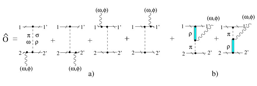
Figure 1: Graphical representation of the scattering operator $\hat{O}(12;1^{\prime}2^{\prime}V)$ (with truncated nucleon lines) for the vector meson production in $NN$ interactions within an effective meson-nucleon theory. The dashed and solid thick lines symbolize the OBE of $\pi,\sigma,\omega,\rho$ mesons with effective parameters listed in Table 1 (see also ref. bonncd ), the wavy lines represent the produced vector meson. The first group of diagrams (a) corresponds to meson production from bremsstrahlung processes, while the last two diagrams (b) depict meson production from the internal conversion of the virtual $\pi\rho$ into real $\omega$ or $\phi$ mesons. The dots symbolize the dressing of the corresponding lines of virtual particles with monopole cut-off form factors.

It is convenient to define for the considered processes an effective scattering operator $\hat{O}(12;1^{\prime}2^{\prime}V)$ which can be derived from the Feynman diagrams for the amplitude by cutting the external nucleon spinors, as depicted in fig. 1, where the external nucleons are represented by solid truncated lines. All the dependencies on meson and nucleon propagators as well as on the polarization of the final meson are included into the definition of $\hat{O}(12;1^{\prime}2^{\prime}V)$. Accordingly, the invariant amplitude $T_{s_{1}s_{2},s_{1}^{\prime},s_{2}^{\prime}}^{{\cal M}_{V}}$ can be obtained by merely sandwiching this operator between the nucleon spinors. For example, for the $pp$ reaction one has

$$T_{s_{1}s_{2},s_{1}^{\prime},s_{2}^{\prime}}^{{\cal M}_{V}}=\left\langle p_{1}^{\prime},s_{1}^{\prime},p_{2}^{\prime},s_{2}^{\prime}\ \left|\ \hat{O}(12;1^{\prime}2^{\prime}V\ \right|\ p_{1},s_{1},p_{2},s_{2}\ \right\rangle-{\rm antisym.}$$ (16)

In the case of $pn$ processes, instead of the antisymmetrization in eq. (16), denoted by ”antisym”, one should properly take into account the isospin factors (see for details ref. titov ). The derivation of the analytical form of the corresponding bremsstrahlung and conversion amplitudes (16) from the Feynman graphs in fig. 1 from the Lagrangians (14) is straightforward but rather cumbersome and we do not present it here. Explicitly the amplitudes $T_{s_{1}s_{2},s_{1}^{\prime},s_{2}^{\prime}}^{{\cal M}_{V}}$ can be found elsewhere, e.g., in ref. titov .

II.2 Effective Parameters

In this subsection we discuss the choice of effective parameters for the bremsstrahlung and conversion processes. The bremsstrahlung diagrams (fig. 1a) consist of two parts, the pure OBE exchange and the emission of the meson from the nucleon lines. The OBE parameters, masses, cut-off’s and coupling constants, are adopted to coincide with those of the OBE potential by the Bonn group with the pseudo-vector coupling in the $\pi NN$ vertex bonncd . Then in the bremsstrahlung part of the amplitude (16) we are left with the parameters of the $VNN$ vertices (vertices with wavy lines in fig. 1a) for the real production of $\omega$ and $\phi$. In principle, the effective parameters for such vertices can differ from the corresponding parametrization of the virtual mesons; consequently in the present work they are considered as free parameters to be fitted independently. For the conversion type vertices $\rho\pi V$ (vertices with wavy lines in fig. 1b) the coupling constant $g_{\rho\pi\omega}$ has been fixed from a systematic study of pseudoscalar and vector meson radiative decays together with the vector meson dominance conjecture (see, e.g. nakayama ; durso ; chung ) and is found to be $g_{\rho\pi\omega}\simeq 12.9\ GeV^{-1}$. ( At this point it is worth mentioning that often in the literature the definition of the coupling constants $g_{\rho\pi V}$ differs from ours in eq. (15) by a mass factor included into $g_{\rho\pi V}$ as to make it dimensionless. So, in refs. nakayama ; dashen this factor reads as $\sqrt{m_{\rho}m_{\omega}}$ which results in a dimensionless coupling constant $g_{\rho\pi\omega}\simeq 10.0$.) The corresponding cut-off parameter, also freely adjustable in the present consideration, has been adjusted to reproduce the angular distribution of $\omega$ mesons from COSY-TOF experiments TOF yielding $\Lambda_{\rho\pi\omega}\simeq 1000\ MeV$. For the $\phi$ production from conversion type diagrams the coupling constant $g_{\rho\pi\phi}$ is adjusted to data for the $\phi\to\rho\pi$ decay. The value $\Gamma(\phi\to\rho\pi)=0.69\ MeV$ suggests $g_{\rho\pi\phi}=-1.1\ GeV^{-1}$ titov (cf. also ref. chung ). Then for the conversion diagram the cut-off parameter $\Lambda_{\rho\pi\phi}$ is found from a combined analysis of the contributions of the conversion and bremsstrahlung diagrams to the experimental cross section DISTO1 ; DISTO2 . Together with the nucleonic cut-off $\Lambda_{N}=720\ MeV$ we adopt $\Lambda_{\rho\pi\phi}=1340\ MeV$, following ref. titov (set ”B”).

Next we explain the choice of parameters for the bremsstrahlung part. Since the nucleon cut-off parameter, $\Lambda_{N}$, has already been fixed, we have now to choose only the coupling constant $g_{\omega NN}$ (and $\kappa_{\omega}$) for the emission of the $\omega$ meson. The corresponding parameters for the $\phi$ meson are connected with symmetry relations with the $\omega$ meson and we do not consider here them as free parameters. The cut-off for $\omega$ meson production as well as for the $\phi$ meson is chosen as in the OBE potential bonncd ($\Lambda_{\phi NN}=\Lambda_{\omega NN}$). In the present work the coupling constant $g_{\omega NN}=9.0$ nakayama is chosen. Then, having fixed the $\omega$ parameters, we find $g_{\phi NN}=-g_{\omega NN}\tan\Delta\theta\simeq-0.8$ with $\Delta\theta\approx 5^{o}\$ okubo77 (cf. also ref. titov ). The parameters used in our calculations are listed in Table 1. It should be noted that the chosen parameters are in the range quoted by eq. (6).

Table 1: Model parameters for the process $NN\to NNV$ ($V=\omega,\phi$).

Vertex		Coupling constant		Cutoff
		($f_{VNN}=\kappa_{V}g_{VNN}$ )		(MeV)
$\rho\pi V$		$g_{\rho\pi\omega}=12.9\ GeV^{-1}$ nakayama ; moya		$\Lambda_{\rho\pi\omega}=980$ nakayama
		$g_{\rho\pi\phi}=-1.1\ GeV^{-1}$ titov ; nakayama1		$\Lambda_{\rho\pi\phi}=1340$ titov
				$\Lambda_{NN}=720$
$VNN$		$g_{\omega NN}=9.$		$\Lambda_{\omega NN}=1500$
		($\kappa_{\omega}=0.5$)
		$g_{\phi NN}=-0.8$ titov		$\Lambda_{\phi NN}=\Lambda_{\omega NN}=1500$
		($\kappa_{\phi}=0.5$, $\Delta\theta\approx 5^{o}$ okubo77 )
$MNN$
$\pi$		$f_{\pi NN}=1.0$		$\Lambda_{\pi NN}=1300$
$\sigma$		$g_{\sigma NN}=10.$		$\Lambda_{\sigma NN}=1800$
$\rho$		$g_{\rho NN}=3.5$		$\Lambda_{\rho NN}=1300$
		($\kappa_{\rho}=6.1$)
$\omega$		$g_{\omega NN}=15.85$		$\Lambda_{\omega NN}=1500$
		($\kappa_{\omega}=0.0$)

II.3 Results for $NN\to NNV$

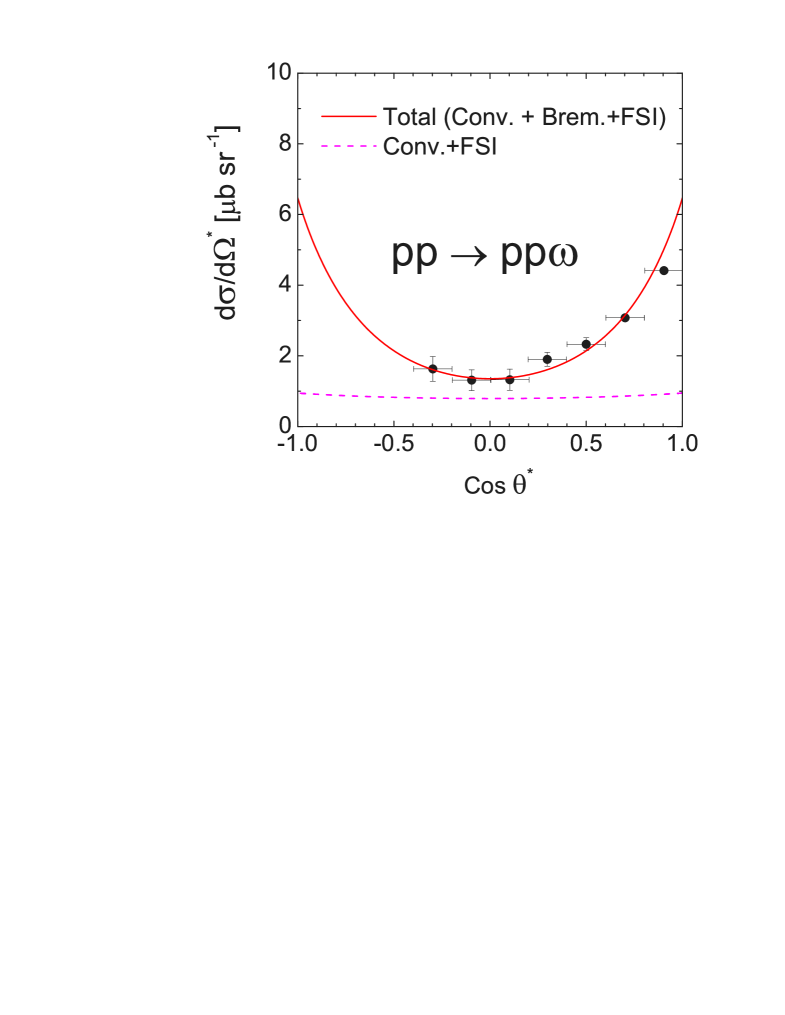
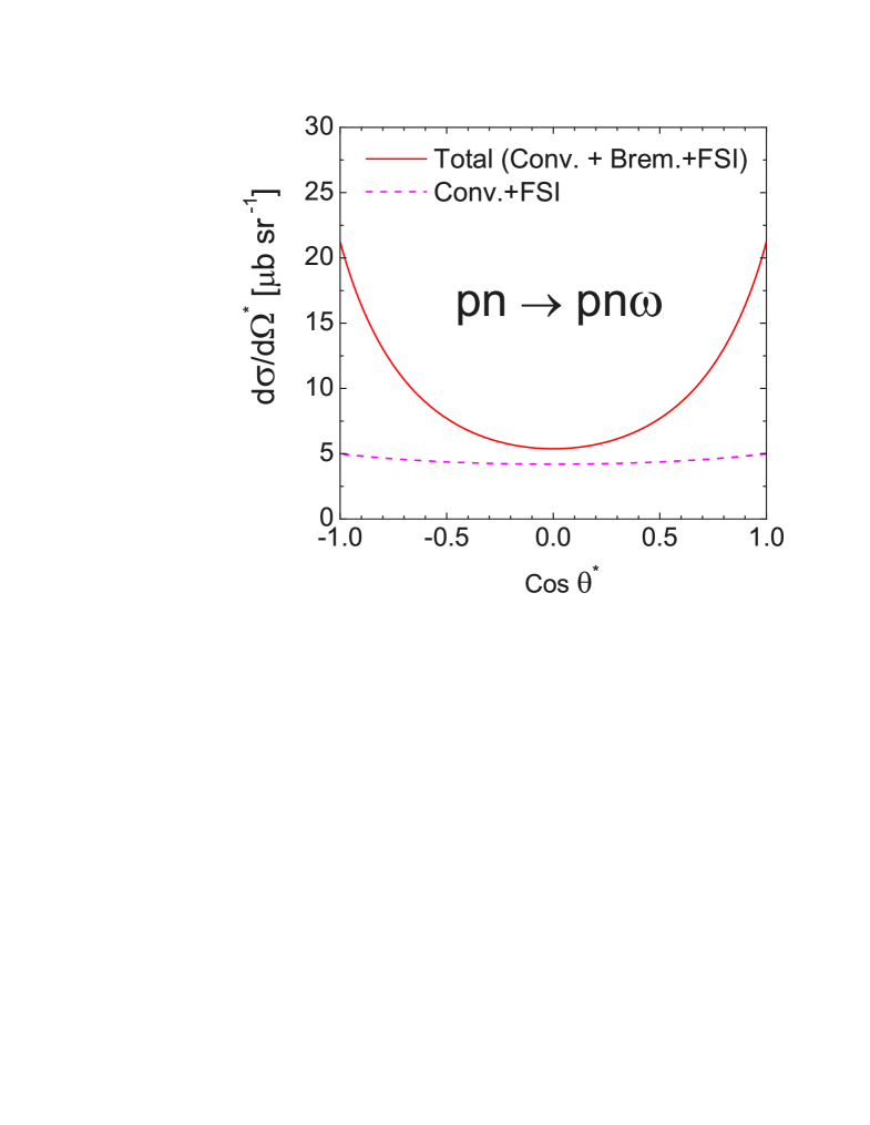
Figure 2: Angular distributions of $\omega$ mesons for the reaction $NN\to NN\omega$ at the excess energy $\Delta s^{\frac{1}{2}}=173\ MeV$. Dashed lines correspond to contributions of conversion currents (fig. 1b), solid lines represent the total contributions of bremsstrahlung and conversion diagrams (figs. 1a and 1b). FSI is included in all contributions. Experimental data are from the COSY-TOF Collaboration TOF .

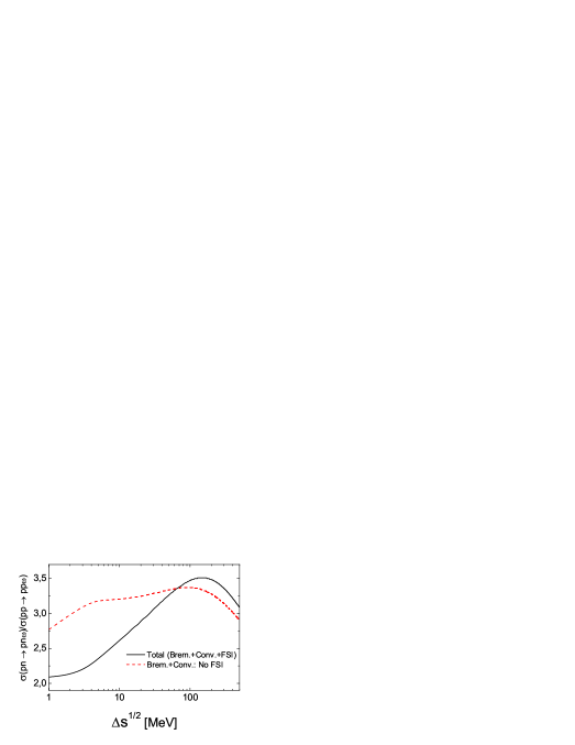
Figure 4: Ratios of the total cross sections of $\omega$ meson production in $pp$ and $pn$ channels as a function of the excess energy. Dashed line denotes the ratio of cross sections without FSI; solid line reflects the ratio of total cross sections with FSI taken into account.

In our calculations we make use of the explicit expressions for the conversion and bremsstrahlung diagrams quoted in ref. titov . The FSI effects have been calculated within the Jost function formalism gillespe which reproduces the singlet and triplet phase shifts at low energies. In fig. 2 we present results of calculations of the angular distribution of $\omega$ mesons at the excess energy $\Delta s^{1/2}=173\ MeV$ ($\Delta s^{1/2}\equiv\sqrt{s}-2m_{p}-m_{V}$) for proton (left panel) and neutron (right panel) targets. The experimental data ankeExper served to fix our free parameters for further calculations of the energy dependence of the total cross section and for an analysis of $pn\to dV$ processes. It can be seen that with the set of parameters listed in Table 1 a good description of the data is achieved. It is also found that the contribution of bremsstrahlung diagrams (fig. 1a) is predominant in both $pp$ and $pn$ processes (see fig. 4). The difference in magnitudes for $pp$ and $pn$ processes is due to the Pauli principle for the former reactions (integration over $d\Omega_{12}^{*}$ in eq. (8) is performed only over one hemisphere of the two protons phase volume) and a possible destructive interference of diagrams due to antisymmetrization effects and isospin enhancements for the latter (see for details ref. titov ).

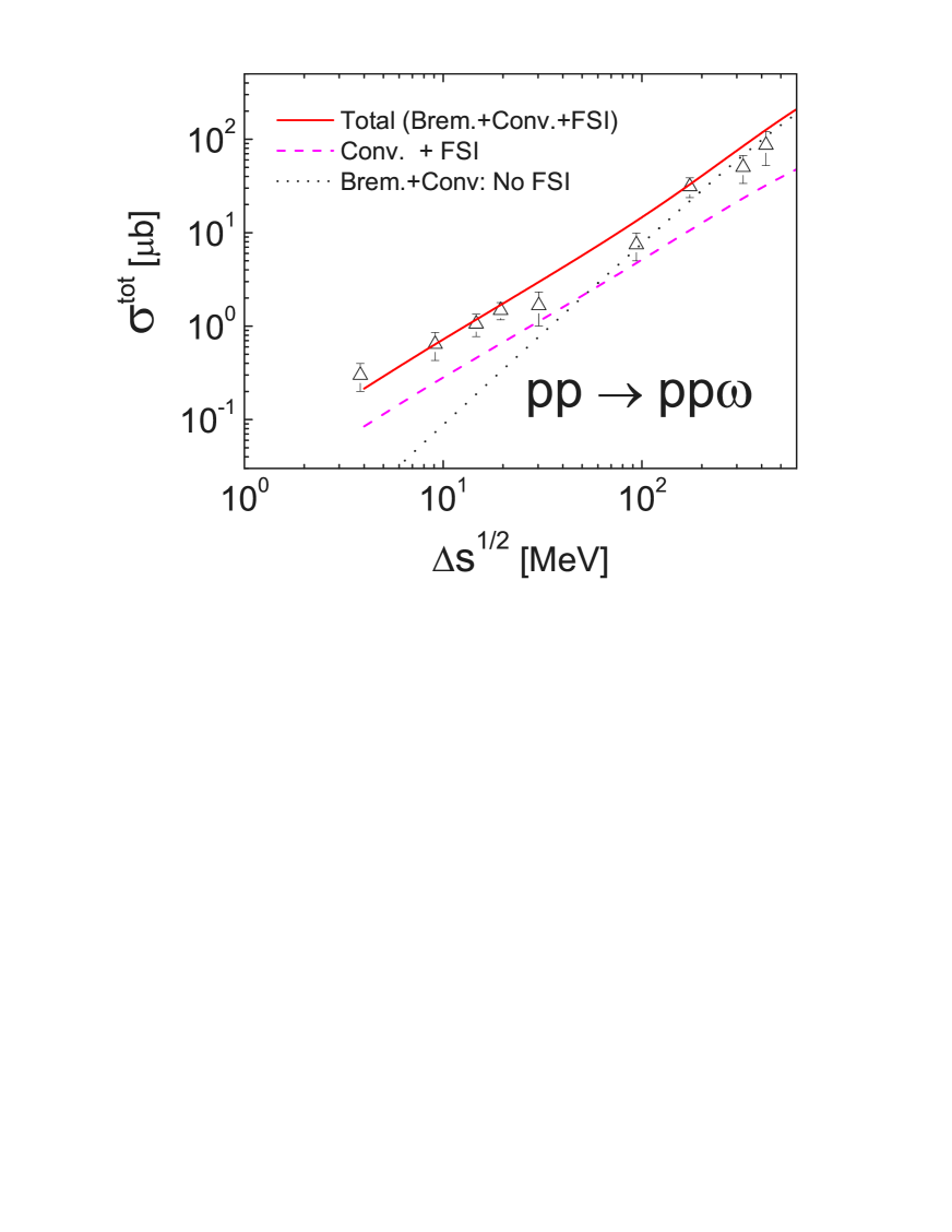
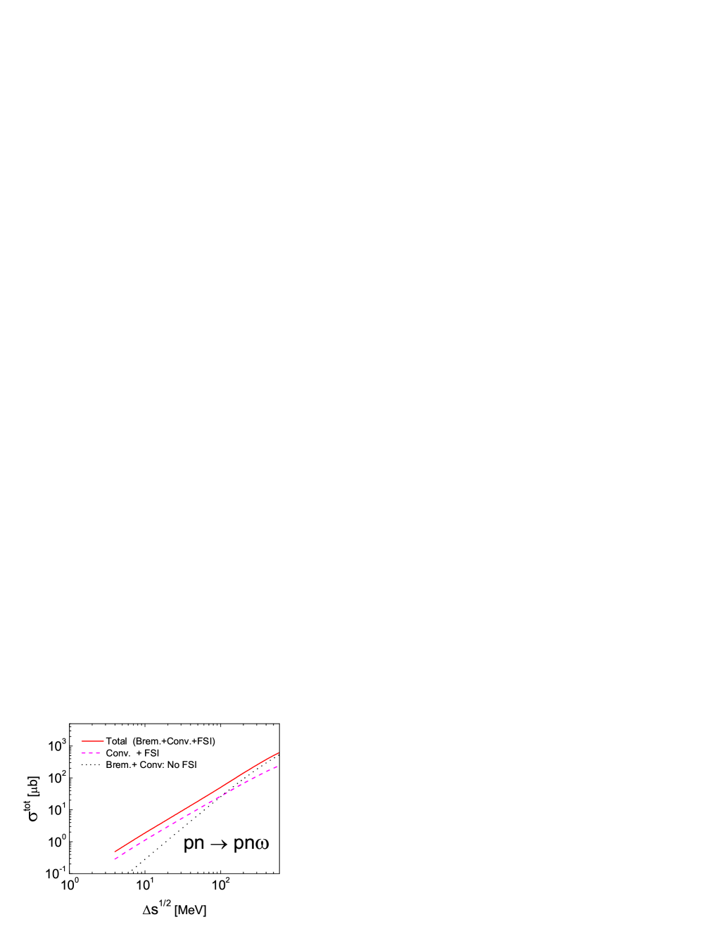
Figure 3: Total cross sections of near-threshold production of $\omega$ mesons in the process $NN\to NN\omega$ (left panel: $pp$ reaction, right panel: $pn$ reaction) as a function of the energy excess $\Delta s^{\frac{1}{2}}=\sqrt{s}-2m_{p}-m_{\omega}$. Dashed lines correspond to contributions of conversion currents solely (fig. 1b), dotted and solid lines represent results with including bremsstrahlung and conversion diagrams (figs. 1a and 1b) without and with FSI effects taken into account, respectively. Experimental data are from SATURNE Hibou , COSY-TOF Collaboration TOF and DISTO Collaboration DISTO1 ; DISTO2 (cf. the compilation in nakayama2 ).

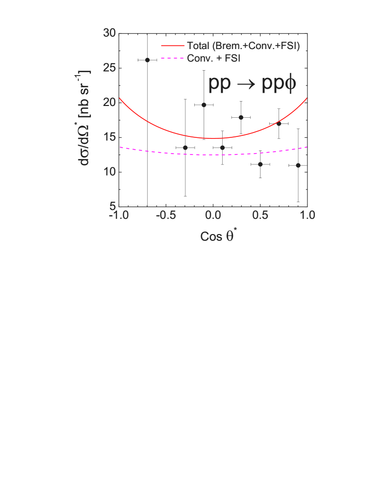
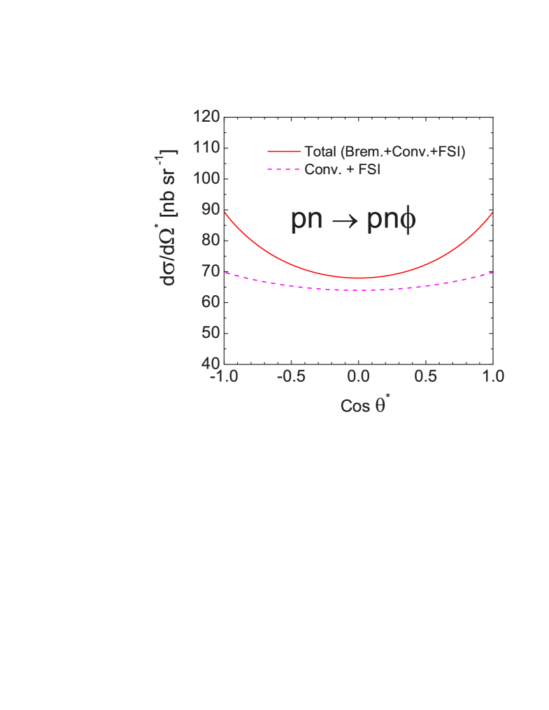
Figure 5: Angular distributions of $\phi$ mesons in the process $NN\to NN\phi$ (left panel: $pp$ reaction, right panel: $pn$ reaction) at the energy excess $\Delta s^{\frac{1}{2}}=83\ MeV$. Experimental data are from the DISTO Collaboration DISTO1 ; DISTO2 . Notation as in fig. 2.

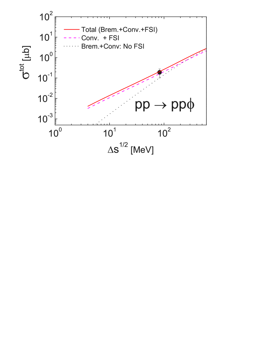
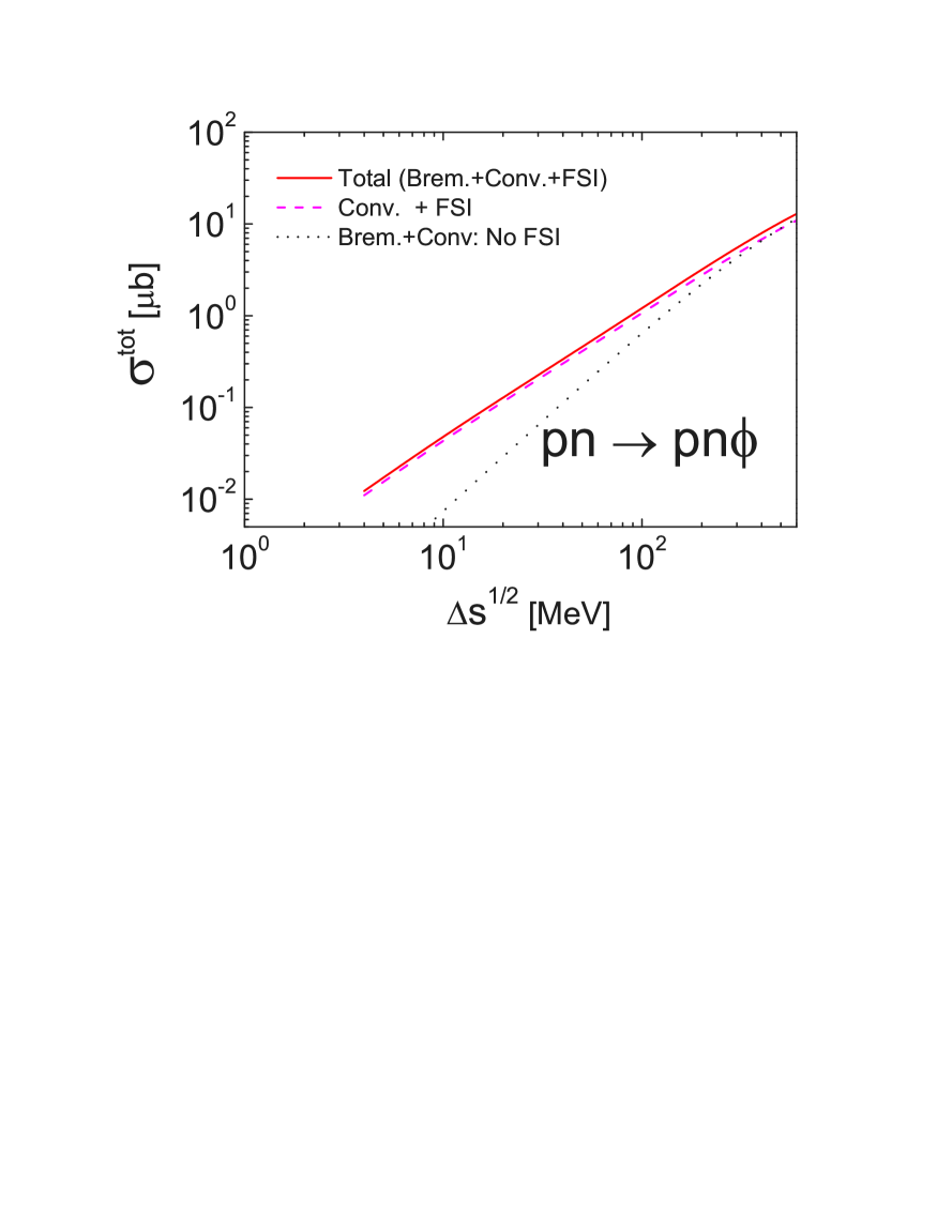
Figure 6: Total cross sections of near-threshold production of $\phi$ mesons in the process $NN\to NN\phi$ as a function of the energy excess $\Delta s^{\frac{1}{2}}=\sqrt{s}-2m_{p}-m_{\phi}$. Experimental data is from the DISTO Collaboration DISTO1 ; DISTO2 . Notation as in fig. 3.

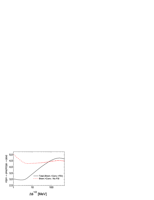
Figure 7: Ratios of the total cross sections of $\phi$ meson production in $pp$ and $pn$ channels. Notation as in fig. 4.

The remaining parameters for $\phi$ have been fixed to describe the data for the angular distribution of $\phi$ production at $\Delta s^{1/2}=83\ MeV$ DISTO1 ; DISTO2 . Having adjusted our parameters in this manner we compute the energy dependence of the total cross section. Results of calculations together with the available experimental data are presented in figs. 3, 5 and 6. The dashed lines represent the contribution of the conversion diagrams alone, the dotted lines are results of calculations of both bremsstrahlung and conversion diagrams by neglecting the FSI effects. Eventually, the solid lines exhibit the total cross section with FSI taken into account titov . A fairly good description of the data in a large interval of the excess energy is achieved. Contrary to $\omega$ production, the contribution of the bremsstrahlung diagram for $\phi$ mesons is much smaller, due to the small value of the $g_{\phi NN}$ coupling. The nontrivial behavior of the ratio $\sigma_{pn\to pnV}/\sigma_{pp\to ppV}$ exhibited in figs. 4 and 7 evidence that the vector meson production cross sections known by $pp$ reactions can not simply be translated into ones for $pn$ reactions. A comparison of the solid and dashed lines in figs. 4 and 7 clearly indicates that near the threshold the FSI in $pp$ and $pn$ systems is different. Rather, a profound analysis, like the one presented here, is needed to have reliable input for simulating heavy-ion and proton-nucleus collisions. This is particularly important for the ongoing experiments with HADES HADES .

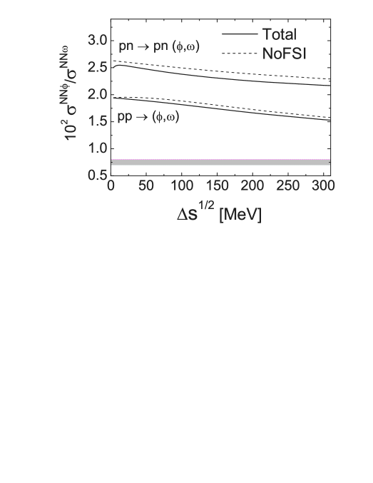
Figure 8: Ratio of the total $\phi$-to-$\omega$ production cross sections in $pp$ and $pn$ reactions. Dashed lines denote the ratio of ”net” cross sections, i.e. without any FSI; solid lines reflect the ratio of total cross sections with FSI taken into account. The shaded area indicates the range of ratios $\left(\displaystyle\frac{g_{\rho\pi\phi}}{g_{\rho\pi\omega}}\right)^{2}\approx 0.0071$ and $\left(\displaystyle\frac{g_{\phi NN}}{g_{\omega NN}}\right)^{2}\approx 0.0079$ (cf. Table 1) used as input for the calculations.

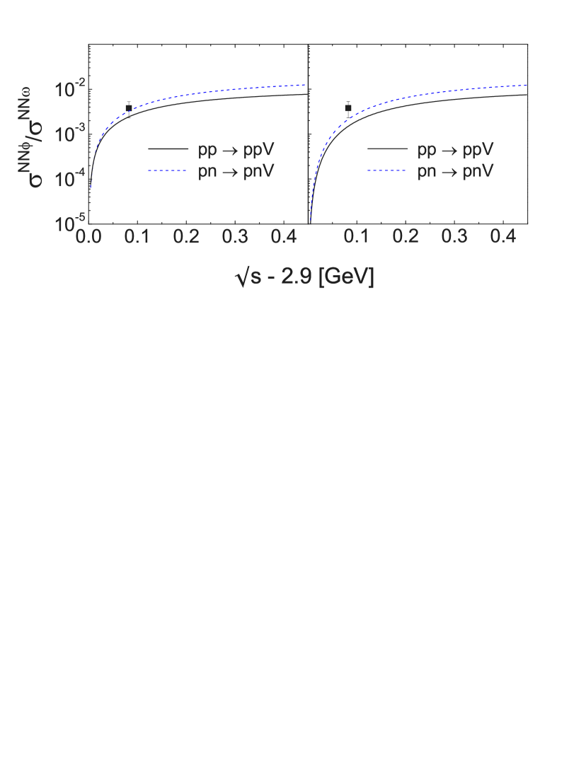
Figure 9: Ratio of the total $\phi$-to-$\omega$ production cross sections in $pp$ (solid lines) and $pn$ (dashed lines) reactions as a function of the excess energy above the $\phi$ threshold. Left (right) panel corresponds to ratio of total cross sections with (without) FSI effects taken into account. Data for the $pp$ reaction is from DISTO Collaboration DISTO2 .

Figures 3 and 6 demonstrate that in the extreme threshold limit the main contribution comes from the final state interaction effects. As the excess energy increases the role of FSI diminishes, even becoming negligible at excess energy $\Delta s^{1/2}>200\ MeV$. This is a disappointing fact, since as mentioned above, the checks of the validity of the OSI rule are preferably to be performed at as low energies as possible (where the loop and double hairpin diagrams are suppressed), while we find that at these energies the ”net” cross section relevant for the OZI rule is completely masked by FSI. However, if the FSI effects can be firmly separated, the total cross section may still serve as criterion of the validity of the OSI rule. This could be estimated by an investigation the OZI $\phi/\omega$ ratio at equal excess energies, where the effects of difference in phase space volumes is minimized, for cross sections with and without including FSI corrections. Figure 8 illustrates that the dependence of such ratios upon the energy is rather weak and practically is not affected by the FSI effects, which let us argue that the adopted Jost method correctly describes the FSI effects. The small difference between ratios with and without FSI can be traced back to the different interactions in $pp$ (${}^{1}S_{0}$ configuration) and $pn$ (${}^{3}S_{1}-{}^{3}D_{1}$ configurations) systems near the threshold. The results in fig. 8 persuade that in this kinematical region the FSI effects, playing an important role in the absolute value of the total cross sections, do not essentially mask the study of OZI rule by ratios of total cross sections. Note that the absolute values of the ratios depicted in fig. 8 clearly indicate a violation of the OZI rule. But this is an apparent effect since the relative contributions of bremsstrahlung and conversion diagrams and, correspondingly, the interference effects are quite different for $\omega$ and $\phi$ production (cf. figs. 3 and 6). Moreover, even at equal excess energies the phase space volumes for $\phi$ and $\omega$ mesons are quite different. Sometimes in the literature one studies the ratio $\phi/\omega$ at equal initial beam energies DISTO1 . In this case one has two effects with opposite contributions: (i) the phase space volume of the $\phi$ meson is much smaller in comparison with the $\omega$ meson (due to different masses, there is a shift of $\sim 240\ MeV$ in $\Delta s^{1/2}$) which will decrease the ratio, and (ii) since at equal beam energies the relative momentum of two produced nucleons is smaller for $\phi$ meson production, the FSI corrections are expected to be larger (cf. figs. 3 and 6). In fig. 9 the OZI ratio at equal beam energies is presented together with data from DISTO1 . It is seen that these ratios are by an order of magnitude smaller than that at equal excess energy and more compatible with the naive OZI rule predictions. In the right panel of fig. 9 the OZI ratio is depicted without any FSI corrections. A comparison with the left panel and with the range of the ratio of input constants (the shaded area in fig. 8) gives some evidence about the magnitude of corrections from the phase space volumes solely.

From the performed analysis one can conclude that an investigation of the OZI rule in $NN\to NNV$ processes near the threshold is feasible, provided one can firmly take into account the FSI effects and, consequently, properly calculate the phase space corrections. The problem of accounting for the FSI between the two nucleons can be solved by considering processes with a definite two-nucleon final state, e.g. the process where the FSI in a $pn$ system result in a bound state, the deuteron.

III The processes $pn\to d\omega$ and $pn\to d\phi$

One way of testing our assertion on the predicted cross sections for $pn$ reactions is to implement them in the tagged quasi-free reaction $pn\to dV$.

III.1 Formalism

Let us consider the reaction

$$p\,+n\,=\,d+V,$$ (17)

where, as before, $V$ denotes the $\omega$ or $\phi$ vector meson and $d$ the deuteron. The invariant differential cross section reads

$$\frac{d\sigma}{dt}=\frac{1}{16\pi\,s(s-4m^{2})}\,\frac{1}{4}\sum\limits_{s_{1},s_{2}}\sum\limits_{{\cal M}_{V},{\cal M}_{d}}\,|T_{s_{1}s_{2}}^{{\cal M}_{V}{\cal M}_{d}}(s,t)|^{2},$$ (18)

where $s$ is the square of the total energy of colliding particles, $t$ is the square of the transferred 4-momentum, $s_{1},s_{2},{\cal M}_{V}$ and ${\cal M}_{d}$ denote the spin projections on a given quantization axis, and $T$ stands for the invariant amplitude of the process (17). As in the previous section the most general form of the amplitude $T$ is presented in the form

$$T_{s_{1}s_{2}}^{{\cal M}_{V}{\cal M}_{d}}(s,t)=\langle D,{\cal M}_{d}\,|\hat{G}_{\mu}\,\xi^{*\mu}_{{\cal M}_{V}}|1,2\rangle,$$ (19)

where $\xi_{{\cal M}_{V}}$ is the polarization vector of the vector meson. The scattering operator $\,\hat{G}\,\,$ represents a vector in the vector space of mesons and a $16\otimes 16$ component object in the spinor space of nucleons; the deuteron is described as a $16$ component BS amplitude $\Phi(1,2)$ which is defined as a matrix element of a time-ordered product of two nucleon fields $\psi(x)$ as

$$\Phi^{\alpha\beta}(1,2)=\langle D|T\left(\psi^{\alpha}(1)\psi^{\beta}(2)\right)|0\rangle$$ (20)

and satisfies the BS equation.

Suppose that in the considered reactions the off-mass shell effects are negligibly small, i.e., the on-mass shell matrix elements of the Lagrangian (15) between real nucleons (reaction (7)) and half-off mass shell matrix elements (reaction (17)) are the same. Then it can be immediately seen that the operator $G^{\mu}\,\xi_{\mu}^{*}$ coincides with the corresponding operator of the process (7), i.e., $\hat{O}=G^{\mu}\,\xi_{\mu}^{*}$. The invariant amplitude may be cast in the form

$$T_{s_{1}s_{2}}^{{\cal M}_{V}{\cal M}_{d}}(s,t)=-i\int\,\frac{d^{4}p}{(2\pi)^{4}}\bar{\Phi}_{{\cal M}_{d}}^{\alpha b}(1^{\prime},2^{\prime})\,\hat{O}^{bc}_{\alpha\beta}(12;1^{\prime}2^{\prime},{\cal M}_{V})u^{c}(1)u^{\beta}(2),$$ (21)

where $\bar{\Phi}_{{\cal M}_{d}}^{ab}(1^{\prime},2^{\prime})$ is the conjugate BS amplitude in the momentum space, $p$ is the relative 4-momentum of the nucleons in the deuteron, and $u(1),u(2)$ denote the Dirac spinors for the incident nucleons. Recall that the operator $\hat{O}^{bc}_{\alpha\beta}(12;1^{\prime}2^{\prime},{\cal M}_{V})$ is a scattering operator describing the vector meson production in the final state. This operator acts in the spinor space of protons and neutrons separately; the upper and lower spinor indices refer to protons and neutrons, respectively. The first indices, $b$ and $\alpha$, form an outer product of two columns, whereas the second ones, $c$ and $\beta$, form an outer product of two rows. To explicitly establish a relation of the amplitude (21) with the corresponding amplitude (16) of the $NN\to NNV$ process we find the spinor structure by a decomposition of the operator $\hat{O}$ in each of its indices over the corresponding complete set of Dirac spinors, i.e,

$$\hat{O}^{bc}_{\alpha\beta}(12;1^{\prime}2^{\prime},{\cal M}_{V})=\frac{1}{(2m)^{4}}\sum\limits_{r,r^{\prime},\rho,\rho^{\prime}=1}^{4}\,A_{r,r^{\prime};\rho,\rho^{\prime}}^{{\cal M}_{V}}(12;1^{\prime}2^{\prime})u^{b}_{r^{\prime}}(1^{\prime})\bar{u}^{c}_{r}(1)\bar{u}^{\beta}_{\rho}(2)u^{\alpha}_{\rho^{\prime}}(2^{\prime}),$$ (22)

where the coefficient $A_{r,r^{\prime};\rho,\rho^{\prime}}^{{\cal M}_{V}}(12;1^{\prime}2^{\prime})$ is determined by the completeness and orthogonality of the Dirac spinors, $\bar{u}_{r}({\bf p})u_{r^{\prime}}({\bf p})=\varepsilon_{r}2m\delta_{rr^{\prime}}$, yielding

$$A_{r,r^{\prime};\rho,\rho^{\prime}}^{{\cal M}_{V}}(12;1^{\prime}2^{\prime})=\varepsilon_{r}\varepsilon_{r^{\prime}}\varepsilon_{\rho}\varepsilon_{\rho^{\prime}}\bar{u}^{b}_{r^{\prime}}(1^{\prime})\,\bar{u}^{\alpha}_{\rho^{\prime}}(2^{\prime})\,\hat{O}^{bc}_{\alpha\beta}(12;1^{\prime}2^{\prime},{\cal M}_{V})u^{c}_{r}(1)\,u^{\beta}_{\rho}(2),$$ (23)

where $\varepsilon=+1$ for $r=1,2$ and $\varepsilon=-1$ for $r=3,4$. Since the defined operator (22) generally acts in the nucleon spinor space its matrix elements describe processes with anti-particles as well. This is explicitly reflected in the dependence of the coefficients $A_{r,r^{\prime};\rho,\rho^{\prime}}^{{\cal M}_{V}}(12;1^{\prime}2^{\prime})$ on spinors with anti-particle quantum numbers. In our case this dependence can occur in the process (17) only as virtual creation and annihilation of $N\bar{N}$ pairs, which within the BS formalism are allowed through the presence of negative-energy $P$ components in the BS amplitude. However, in the considered kinematics the contribution of $P$ waves is by far smaller than the main $S^{++}$ and $D^{++}$ components quad and consequently, in what follows we disregard all the partial BS amplitudes with at least one negative energy index, leaving only the $S^{++}$ and $D^{++}$ waves. Then substituting (22) into (21) one obtains

$$T_{s_{1}s_{2}}^{{\cal M}_{V}{\cal M}_{d}}(s,t)=\frac{-i}{(2m)^{2}}\int\,\frac{d^{4}p}{(2\pi)^{4}}\bar{\Phi}_{{\cal M}_{d}}^{\alpha b}(1^{\prime},2^{\prime})\,\sum\limits_{rr^{\prime}=1}^{2}A_{s_{1}s_{2};rr^{\prime}}^{{\cal M}_{V}}(12;1^{\prime}2^{\prime})u^{\alpha}_{r^{\prime}}(2^{\prime})u^{b}_{r}(1^{\prime})$$

$$=\frac{i}{(2m)^{2}}\sum\limits_{rr^{\prime}=1}^{2}\int\,\frac{d^{4}p}{(2\pi)^{4}}\left(u^{\alpha}_{r^{\prime}}(2^{\prime})\right)^{T}\gamma_{c}^{\alpha\alpha^{\prime}}\left(\gamma_{c}^{\alpha^{\prime}\alpha^{\prime\prime}}\bar{\Phi}_{{\cal M}_{d}}^{\alpha^{\prime\prime}b}(1^{\prime},2^{\prime})\right)\,A_{s_{1}s_{2};rr^{\prime}}^{{\cal M}_{V}}(12;1^{\prime}2^{\prime})u^{b}_{r}(1^{\prime})$$

$$=\frac{i}{(2m)^{2}}\sum\limits_{rr^{\prime}=1}^{2}\int\,\frac{d^{4}p}{(2\pi)^{4}}A_{s_{1}s_{2};rr^{\prime}}^{{\cal M}_{V}}(12;1^{\prime}2^{\prime})\bar{v}_{r^{\prime}}(2^{\prime})\bar{\Psi}_{{\cal M}_{d}}(1^{\prime},2^{\prime})u_{r}(1^{\prime}),$$ (24)

where $\gamma_{c}$ is the charge conjugation matrix, $\bar{v}_{r}(2^{\prime})\equiv u^{T}_{r}(2^{\prime})\gamma_{c}$, and the new BS amplitude $\bar{\Psi}_{{\cal M}_{d}}(1^{\prime},2^{\prime})\equiv\gamma_{c}\bar{\Phi}_{{\cal M}_{d}}(1^{\prime},2^{\prime})$ is written now in the form of a $4\otimes 4$ matrix and represents the solution of the BS equation written also in matrix form. Note that in eq. (24) the spinor $\bar{v}_{r^{\prime}}(2^{\prime})$ does not describe an anti-particle, it is rather a consequence of the efforts made to cast the BS amplitude in a matrix form (see for details, e.g., refs. Tjon ) and still refers to nucleons.

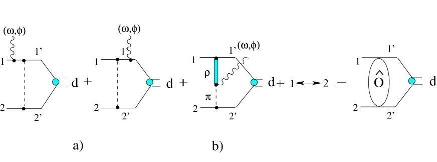
Figure 10: Diagrams contributing to the process $pn\to dV$. The sum of bremsstrahlung (a) and conversion-type (b) diagrams results in the matrix element of the operator $\hat{O}(12;1^{\prime}2^{\prime}V)$ (fig. 1) sandwiched between the initial two-nucleon states and the final deuteron.

As in the previous case of $NN$ reactions, the effective interactions in eq. (15) again result into two types of diagrams, conversion currents and bremsstrahlung emission, which are depicted in fig. 10. Consequently, having already computed the operator $\hat{O}$, it is straightforward to obtain the coefficients $A_{r,r^{\prime};\rho,\rho^{\prime}}^{M_{V}}(12;1^{\prime}2^{\prime})$ in eq. (23) within the OBE approximation. Note that in case when all particles are on mass shell, $A_{r,r^{\prime};\rho,\rho^{\prime}}^{M_{V}}(12;1^{\prime}2^{\prime})$ exactly coincides with the amplitude (16) of the elementary process (7), i.e., $A_{r,r^{\prime};\rho,\rho^{\prime}}^{M_{V}}(12;1^{\prime}2^{\prime})=T_{r,r^{\prime};\rho,\rho^{\prime}}^{{\cal M}_{V}}(12;1^{\prime}2^{\prime}V)$. However, in general this amplitude corresponds to a virtual process of vector meson production with two off-mass shell nucleons in the final state.

Since our numerical solution for the BS equation has been obtained in the deuteron center of mass solution , all further calculations will be performed in this system. First we introduce the relevant kinematical variables as follows: $p_{1}$ and $p_{2}$ are the four momenta of incoming nucleons, $p_{1}^{\prime}$ and $p_{2}^{\prime}$ stand for the momenta of the internal (off-mass shell) nucleons in the deuteron with $p=(p_{1}^{\prime}-p_{2}^{\prime})/2$, $\xi_{\cal M}$ denotes the polarization 4-vectors of the deuteron and vector mesons. In this notation the BS amplitudes in the deuteron rest system are of the form quad

$$\!\!\!\!\!\Psi_{{\cal M}_{d}}^{S^{++}}(p_{1}^{\prime},p_{2}^{\prime})={\cal N}(\hat{k}_{1}+m)\frac{1+\gamma_{0}}{2}\hat{\xi}_{{\cal M}_{d}}(\hat{k}_{2}-m)\phi_{S}(p_{0},|{\bf p}|),$$ (25)

$$\!\!\!\!\!\Psi_{{\cal M}_{d}}^{D^{++}}(p_{1}^{\prime},p_{2}^{\prime})=-\frac{{\cal N}}{\sqrt{2}}(\hat{k}_{1}+m)\frac{1+\gamma_{0}}{2}\left(\hat{\xi}_{{\cal M}_{d}}+\frac{3}{2|{\bf p}|^{2}}(\hat{k}_{1}-\hat{k}_{2})(p\xi_{M})\right)(\hat{k}_{2}-m)\phi_{D}(p_{0},|{\bf p}|),$$

where $k_{1,2}$ are on-mass shell 4-vectors related to the off-mass shell vectors $p_{1,2}^{\prime}$ as follows

$$k_{1}=(E_{\bf p},{\bf p}),\quad k_{2}=(E_{\bf p},-{\bf p}),\quad p_{1}^{\prime}=(p_{10}^{\prime},{\bf p}),\quad p_{2}^{\prime}=(p_{20}^{\prime},-{\bf p}),\quad E_{\bf p}=\sqrt{{\bf p}^{2}+m^{2}},$$

and $\phi_{S,D}(p_{0},|{\bf p}|)$ are the partial scalar amplitudes, related to the corresponding partial vertices as

$$\phi_{S,D}(p_{0},|{\bf p}|)=\displaystyle\frac{G_{S,D}(p_{0},|{\bf p}|)}{\left(\displaystyle\frac{M_{D}}{2}-E_{\bf p}\right)^{2}-p_{0}^{2}}.$$

$M_{d}$ is the deuteron mass, and the normalization factor reads ${\cal N}=\displaystyle\frac{1}{\sqrt{8\pi}}\displaystyle\frac{1}{2E_{\bf p}(E_{\bf p}+m)}$. The components of the polarization vector of a vector particle moving with 4-momentum $p=(E,{\bf p})$, having the polarization projection ${\cal M}=\pm 1,\,0$ and mass $M$ are

$$\xi_{\cal M}=\left(\frac{\bf p{\mathchar 28952\relax}_{\cal M}}{M},{\mathchar 28952\relax}_{\cal M}+{\bf p}\frac{\bf p{\mathchar 28952\relax}_{\cal M}}{M(E_{\bf p}+M)}\right),$$ (26)

where ${\mathchar 28952\relax}_{\cal M}$ is the polarization vector for the particle at rest,

$$\begin{array}[]{ccc}{\mathchar 28952\relax}_{+1}=-\displaystyle\frac{1}{\sqrt{2}}\,\left(\begin{array}[]{c}1\\ i\\ 0\end{array}\right),&\quad{\mathchar 28952\relax}_{-1}=\displaystyle\frac{1}{\sqrt{2}}\left(\begin{array}[]{c}1\\ -i\\ 0\end{array}\right),&\quad{\mathchar 28952\relax}_{0}=\left(\begin{array}[]{c}0\\ 0\\ 1\end{array}\right).\end{array}$$ (27)

The Dirac spinors, normalized as $\bar{u}(p)u(p)=2m$ and $\bar{v}(p)v(p)=-2m$, read

$$u({\bf p},s)=\sqrt{m+E_{{\bf p}}}\left(\begin{array}[]{c}\chi_{s}\\ \displaystyle\frac{{\mathchar 28955\relax}{\bf p}}{m+E_{{\bf p}}}\chi_{s}\end{array}\right),\quad\quad v({\bf p}\,,s)=\sqrt{m+E_{{\bf p}}}\left(\begin{array}[]{c}\displaystyle\frac{{\mathchar 28955\relax}{\bf p}}{m+E_{{\bf p}}}\widetilde{\chi}_{s}\\ \widetilde{\chi}_{s}\end{array}\right),$$ (32)

where $\widetilde{\chi}_{s}\equiv-i\sigma_{y}\chi_{s}$, and $\chi_{s}$ denotes the usual two-dimensional Pauli spinor. In general, the BS amplitude consists on eight partial components. As already mentioned, in eq. (25) we take into account only the most important ones, namely the $S$ and $D$ partial amplitudes. The other six amplitudes may become important at high transferred momenta ourphysrev ; quad , hence for the present near-threshold process (17) they may be safely disregarded. Substituting eqs. (25)-(32) into (24) one obtains after some algebra ourPhi

$$\!\!\!\!\!\!\!\!T_{s_{1}s_{2}}^{{\cal M}_{V}{\cal M}_{d}}(s,t)=\frac{-i}{\sqrt{8\pi}}\sqrt{|{\cal M}_{d}|+1}$$

$$\!\!\!\!\!\!\!\!\times\sum\limits_{rr^{\prime}}\int\,\frac{d^{4}p}{2E_{\bf p}(2\pi)^{4}}\frac{G_{S}-G_{D}/\sqrt{2}}{\left(M_{D}/2-E_{\bf p}\right)^{2}-p_{0}^{2}}A_{s_{p},s_{n};rr^{\prime}}^{{\cal M}_{V}}({\bf p}_{1},{\bf p}_{2};{\bf p}_{1}^{\prime},{\bf p}_{2}^{\prime},{\bf P}_{V})\delta_{r+r^{\prime};{\cal M}_{d}}$$ (33)

$$\!\!\!\!\!\!\!\!+\frac{3i}{\sqrt{16\pi}}\sum\limits_{rr^{\prime}}\int\,\frac{d^{4}p}{2E_{\bf p}(2\pi)^{4}}\frac{G_{D}}{\left(M_{D}/2-E_{\bf p}\right)^{2}-p_{0}^{2}}A_{s_{p},s_{n};rr^{\prime}}^{{\cal M}_{V}}({\bf p}_{1},{\bf p}_{2};{\bf p}_{1}^{\prime}{\bf p}_{2}^{\prime}{\bf P}_{\phi})\widetilde{\chi}^{+}_{r^{\prime}}\,({\mathchar 28955\relax}{\mbox{\boldmath$n$}})\chi_{r}\,({\mbox{\boldmath$n$}}{\mathchar 28952\relax}^{*}_{{\cal M}_{d}}).$$

By closing the integration contour in the upper hemisphere and picking up the residuum in $p_{0}=M_{d}/2-E_{\bf p}$ and introducing the notion of the deuteron $S$ and $D$ wave functions as

$$u_{S}(p)=\frac{G_{S}(p_{0},|{\bf p}|)/4\pi}{\sqrt{2M_{D}}(2E_{\bf p}-M_{d})};\quad u_{D}(p)=\frac{G_{D}(p_{0},|{\bf p}|)/4\pi}{\sqrt{2M_{D}}(2E_{\bf p}-M_{d})};$$

$${\rm with}\qquad\frac{2}{\pi}\int|{\bf p}|^{2}\,d\,|{\bf p}|(u_{S}^{2}+u_{D}^{2})\approx 1,$$ (34)

the final expression for the amplitude $T$ may be cast in the form

$$T_{s_{1}s_{2}}^{{\cal M}_{V}{\cal M}_{d}}(s,t)=\sqrt{\frac{M_{D}}{4\pi}}\sum\limits_{rr^{\prime}}\int\,\frac{d^{3}{\bf p}}{E_{p}(2\pi)^{2}}A_{s_{p},s_{n};rr^{\prime}}^{{\cal M}_{V}}({\bf p}_{1},{\bf p}_{2};{\bf p},-{\bf p},{\bf P}_{V})$$

$$\times\left\{\sqrt{|{\cal M}_{d}|+1}\left[u_{S}(p)-\frac{u_{D}(p)}{\sqrt{2}}\right]\delta_{r+r^{\prime};{\cal M}_{d}}-3\frac{u_{D}(p)}{\sqrt{2}}\left({\mathchar 28952\relax}^{*}_{{\cal M}_{d}}{\mbox{\boldmath$n$}}\right)\,\widetilde{\chi}_{r^{\prime}}({\mathchar 28955\relax}{\mbox{\boldmath$n$}})\chi_{r}\right\},$$ (35)

where $n$ is a unit vector parallel to ${\bf p}$. Equation (35) may be written in a more familiar form as to better emphasize the relation of our formulae with their non-relativistic analogues. For this sake observe that in eq. (35) one has $\sqrt{|{\cal M}_{d}|+1}\delta_{r+r^{\prime};{\cal M}_{d}}=-\sqrt{2}\langle\frac{1}{2}\ r\frac{1}{2}r^{\prime}|1{\cal M}_{d}\rangle$ and $\left({\mathchar 28952\relax}^{*}_{{\cal M}_{d}}{\mbox{\boldmath$n$}}\right)\,({\mathchar 28955\relax}{\mbox{\boldmath$n$}})=(4\pi/3)\sum\limits_{\alpha,\beta}(-1)^{\alpha+\beta}{\mathchar 28952\relax}^{*}_{-\alpha}{\mathchar 28955\relax}_{-\beta}{\rm Y}_{1\alpha}({\mbox{\boldmath$n$}}){\rm Y}_{1\beta}({\mbox{\boldmath$n$}})$, where ${\rm Y_{lm}}({\mbox{\boldmath$n$}})$ are the usual spherical harmonics. Then, by making use of the addition theorem for the spherical harmonics ${\rm Y_{lm}}({\mbox{\boldmath$n$}})$ and the Wigner-Eckart theorem for the matrix elements between states with definite angular momenta, the amplitude $T_{s_{1}s_{2}}^{{\cal M}_{V}{\cal M}_{d}}(s,t)$ becomes

$$T_{s_{1}s_{2}}^{{\cal M}_{V}{\cal M}_{d}}(s,t)=\sqrt{2M_{D}}\sum\limits_{rr^{\prime}}\int\,\frac{d^{3}{\bf p}}{E_{p}(2\pi)^{2}}A_{s_{p},s_{n};rr^{\prime}}^{{\cal M}_{V}}({\bf p}_{1},{\bf p}_{2};{\bf p},-{\bf p},{\bf P}_{V})\times$$ (36)

$$\left\{\left\langle\frac{1}{2}r\frac{1}{2}r^{\prime}|1{\cal M}_{d}\right\rangle{\rm Y_{00}}({\mbox{\boldmath$n$}})u_{S}(p)-\sum\limits_{{\rm m},\nu_{12}}\left\langle 2{\rm m}1\nu_{12}|1{\cal M}_{d}\right\rangle\left\langle\frac{1}{2}r\frac{1}{2}r^{\prime}|1\nu_{12}\right\rangle{\rm Y_{2m}^{*}}({\mbox{\boldmath$n$}})u_{D}(p)\right\},$$

where the last line exactly coincides with a non-relativistic spin overlap between the deuteron wave function and two Pauli spinors of intermediate nucleons. Note that usually in non-relativistic meson-nucleon theories the analogue of the amplitude $T_{s_{1}s_{2}}^{{\cal M}_{V}{\cal M}_{d}}(s,t)$ is obtained by a non-relativistic reduction of the initially covariant operator $\hat{O}$ with subsequent calculations of the matrix element

$$T_{s_{1}s_{2}}^{{\cal M}_{V}{\cal M}_{d}\ N.R.}(s,t)=\left\langle D,{\cal M}_{d}\left|\,\hat{O}^{N.R.}(12;1^{\prime}2^{\prime}V)\,\right|{\bf p}_{1},s_{1},{\bf p}_{2},s_{2}\right\rangle$$

$$=\sum\limits_{r,r^{\prime}=1}^{2}\left\langle D,{\cal M}_{d}\ |k_{1},r,k_{2},r^{\prime}\right\rangle\langle k_{1},r,k_{2},r^{\prime}\ |\hat{O}^{N.R.}(12;1^{\prime}2^{\prime}V)\ |{\bf p}_{1},s_{1},{\bf p}_{2},s_{2}\rangle,$$ (37)

where now $\left\langle D,{\cal M}_{d}\ |k_{1},r,k_{2},r^{\prime}\right\rangle$ is the non-relativistic (complex conjugated) deuteron wave function in the momentum space. In our case, the use of the BS formalism allows to compute the matrix element (36) directly from the covariant expression of the previously found operator $\hat{O}$, avoiding the cumbersome procedure of its non-relativistic reduction for non-relativistic calculations by eq. (37). However, since in the considered kinematical range the BS wave functions, eq. (34), are rather similar to their non-relativistic analogues (see, e.g. quad ) and due to the formal equivalence of eqs. (36) and (37) we can use the former one for non-relativistic calculations as well by merely replacing $u_{S}(p)$ and $u_{D}(p)$ with the corresponding quantities from the Schrödinger equation with, e.g., Bonn or Paris potentials.

III.2 Results for $pn\to dV$

In our calculation of the cross section of the process (17) we use the numerical solution of the BS equation solution in ladder approximation obtained with a realistic OBE interaction. The effective parameters used in the ladder approximation when solving the BS equation have been fixed in such a way to obtain a good description of the $NN$ elastic scattering data and the main static properties of the deuteron quad . The obtained parameters turn out to be very close to those obtained in the non-relativistic framework of the Bonn group in determining the OBE $NN$ potential bonncd . In this sense our analysis of the processes with the deuteron is consistent with the previous consideration of $NN\to NNV$ processes.

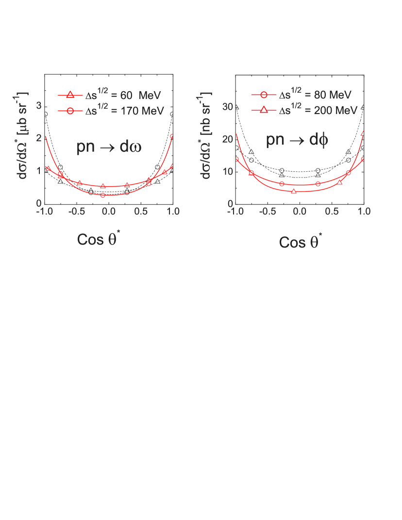
Figure 11: Angular distributions for $\omega$ (left panel) and $\phi$ (right panel) mesons produced in $pn\to dV$ processes for various values of the excess energy $\Delta s^{1/2}=\sqrt{s}-M_{d}-m_{V}$ ($V=\omega,\phi$). Solid lines: results of calculations with the deuteron wave function obtained within the BS formalism; dashed lines: the non-relativistic deuteron wave function with the Bonn potential. The curves labelled with open circles correspond to values of $\Delta s^{1/2}$ for which the experimental data of elementary process $pp$ exits (cf. figs. 2-6); the curves labelled with triangles are presented for an illustration of the change of the distributions with the excess energy.

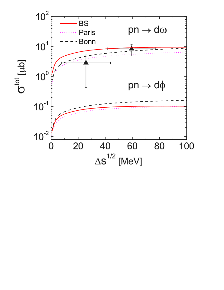
Figure 12: Total cross sections for $\omega$ and $\phi$ mesons for $pn\to dV$ reactions as a function the excess energy $\Delta s^{\frac{1}{2}}=\sqrt{s}-M_{d}-m_{V}$ ($V=\omega,\phi$). Solid lines: results of calculations with the deuteron wave function obtained within the BS formalism; dashed (dotted) lines: using the non-relativistic deuteron wave function with the Bonn (Paris) potential. The experimental data are from COSY-ANKE ankeExper .

In figs. 11 and 12 the angular distribution and the total cross section are depicted. The shape of our evaluated cross section is rather similar to one computed in ref. nakayama . However, there is some difference in the absolute values in case of $\phi$. This difference is probably due to the fact that we fitted our parameters to $\pi N\to\phi N$ data and to $NN\to\phi NN$ data, in particular, the new DISTO data point with $\sigma=0.17\ \mu b$ DISTO2 . In addition, the methods of calculating the FSI effects are slightly different, which could provide some difference in values of FSI corrections as well. Nevertheless, the magnitude of our parameters and those of ref. nakayama are very close to each other. It is also worth emphasizing that, as discussed in refs. titov ; nakayama , there can be several sets of parameters equally well describing the $pp\to ppV$ data. These sets differ not only by absolute values of parameters but also by the relative contributions of bremsstrahlung and conversion diagrams which possess different isospin structure and, hence differently contribute to $pp$ and $pn$ processes. So, in case of $pn\to dV$ processes the isospin transition corresponds to $\Delta{\cal T}=0$, consequently the conversion diagrams are enhanced by a factor of ”-3” in comparison with the bremsstrahlung diagram with exchange of neutral mesons. That means that (i) the contributions of bremsstrahlung terms are strongly reduced in $pn\to dV$ processes in comparison with the elementary $pp$ reaction and (ii) the shape of the cross sections and angular distributions in the process $pn\to dV$ follows the behavior of the corresponding distribution in the elementary processes, modified by the deuteron wave function. This is clearly seen in fig. 11, where the shape of the angular distribution is very similar to the distributions found in $pn$ reactions (the shapes of the corresponding distributions in figs. 2 and 5 must be compared with the curves labelled by open circles in fig. 11). At the threshold the distribution is fairly flat, while with increasing energy some structure around the forward-backward directions becomes pronounced. The shape of the differential cross section in near forward and backward directions depends essentially upon the parameter set used in calculations (for a detailed analysis of the dependence of the shape of the angular distributions upon the chosen parameters, see nakayama1 ; nakayama2 ).

In fig. 12 the total cross sections for $\omega$ and $\phi$ meson production are depicted as a function of the excess energy. The $\omega$ production is larger than the $\phi$ cross section by roughly two orders of magnitude. From figs. 11 and 12 we observe that the computed cross sections exhibit a dependence on the potential used in the calculations of the deuteron wave function. This dependence is more pronounced at relatively low energies and has opposite behavior in $\omega$ (the BS wave function provides slightly larger cross sections than the Bonn one) and $\phi$ production (the BS cross section is smaller than the Bonn one). This difference decreases with increasing energy. This can be observed from a comparison of angular distributions at two different energies (compare the curves labelled with open circles with the ones labelled by triangles in fig. 11). In fig. 12 this effect is seen for $\omega$ production (the upper panel) and not yet visible for $\phi$ mesons (lower panel).

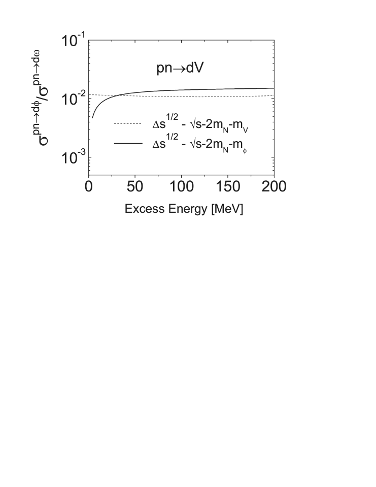
Figure 13: The OZI rule ratio for $pn\to dV$ processes as a function of the excess energy. The dashed line represents the ratio at equal values of the excess energy, while the solid line reflects the ratio at equal beam energies and is measured from the threshold of $\phi$ meson production.

Eventually, in fig. 13 we analyze the values of the OZI ratio defined at equal excess energies (dashed line) and at equal beam energies (solid line). Corresponding to our approach in both cases the FSI effects are the same (i.e., the deuteron in the final state). The only difference should appear due to the difference in the phase space volumes for $\omega$ and $\phi$ mesons which is estimated to be minimized for the ratio at equal excess energy near the threshold and more pronounced for the ratio at equal beam energies. As the energy increases the difference in the two definitions should not be too large, as seen in fig. 13. In both cases the OZI ratio is essentially larger than the one expected form the naive OZI rule restrictions.

IV Summary

In summary we present a combined analysis of vector meson production in $pp\to ppV$, $pn\to pnV$ and $pn\to dV$ processes for $V=\omega,\phi$. The elementary reactions $NN$ are treated within an effective meson-nucleon theory with most parameters fixed from independent experiments. The few remaining parameters are fitted to achieve a reasonably good description of the available angular distributions. With these parameters at our disposal we obtain a fairly good description of the energy dependence of total cross sections. Then the OZI rule is analyzed for different definitions of the relevant ratio of $\phi/\omega$ meson production. It is found that an enhancement of the OZI rule ratios can be obtained without any expected violation of the original rule and could be interpreted as dynamical effect which occurs as a sophisticated interference of different types of diagrams and isospin effects. Using the same meson-nucleon theory we investigate vector production with a deuteron in the final state. In order to be able to use directly the results from elementary reaction we apply the Bethe-Salpeter formalism for the deuteron in the final state. The final expressions are presented in a form fully corresponding to the non-relativistic approach. Calculations with the same set of parameters show that within the proposed approach one can obtain reasonable values of the total cross section, close to the preliminary experimental data from ANKE. The OZI rule ratio is found to be almost independent of the energy and, similarly to the $NN$ case, is enhanced relative to the naive expectations, based on the OZI rule restrictions.

The proposed approach allows to calculate a number of polarization observables in the considered processes which could be directly related with the OZI rule. However this task is beyond of the goal of the present paper. An analysis of polarization observables in $NN\to NN\phi$ reactions can be found in ref. titov and a for $pn\to d\phi$ in ref. ourPhi .

Our approach extends the study of nakayama2 by including the neutron channels and the deuteron final state. First experimental data for $pn\to d\omega$ is at our disposal, while for $pn\to d\phi$ data are expected soon from COSY-ANKE. It should be noted that in nakayama2 also a few nucleon resonances are taken into account for $\omega$. This leads to a renormalization of parameters, coupling constants and cut-off’s, and invokes further new parameters. The role of baryon resonances is, in particular, stressed in Fuchs2 . The comprehensive extension of our approach with inclusion of the full list of resonances deserves a separate investigation, e.g. along the lines of Mosel ; M.Lutz ; Sasha .

Acknowledgements

We thank H.W, Barz, A.I. Titov, S.S. Semikh for useful discussions. L.P.K. would like to thank for the warm hospitality in the Research Center Rossendorf. This work has been supported by the BMBF grant 06DR121.

References

-
(1)
S. Okubo, Phys. Lett. 5 (1963) 165;
G. Zweig, CERN Report 8419/TH 412 (1964);
I. Iizuka, Prog. Theor. Phys. Suppl. 37/38 (1966) 21. - (2) J.J. Sakurai, Phys. Rev. Lett. 9 (1962) 472.
- (3) M. Gell-Mann, Phys. Rev. 125 (1962) 1067.
- (4) S. Okubo, Phys. Rev. D 16 (1977) 2336.
- (5) F. Balestra at al. (DISTO Collaboration), Phys. Rev. Lett. 81 (1998) 4572.
- (6) F. Balestra at al. (DISTO Collaboration) Phys. Rev. C 63 (2001) 024004; Phys. Lett. B 468 (1999) 7.
-
(7)
R. Bilger et al., Nucl. Inst. Meth. A 457 (2001) 64;
H. Calen et al., Phys. Rev. Lett. 80 (1998) 2069. - (8) M. Büscher et al., ”Study of and meson production in the reaction at ANKE, Exp. #75/ANKE.
- (9) A. Sibirtsev, W. Cassing, Eur. Phys. J. A 7 (2000) 407.
- (10) J.R. Ellis, M. Karliner, D.E. Kharzeev, M.G. Sapozhnikov, Nucl. Phys. A 673 (2000) 256; Phys. Lett. B 353 (1995) 319.
-
(11)
V.E. Markushin, M.P. Locher, Eur. Phys. J. A 1 (1998) 91;
S. von Rotz, M.P. Locher, V.E. Markushin, hep-ph/9912359. - (12) J.F. Donoghue, C.R. Nappi, Phys. Lett. B 168 (1986) 105.
- (13) J. Gasser, H. Leutwyler, M.E. Sainio, Phys. Lett. B 253 (1991) 252.
- (14) J. Ashman et al., Phys. Lett. B 206 (1988) 364.
- (15) N. Isgur, H.B. Thacker, hep-lat/0005006 (2000); Phys. Rev. D 64 (2001) 094507.
- (16) T. Schäfer, E.V. Shuryak, hep-lat/0005025.
- (17) L.A. Kondratyuk, Ye. Golubeva, M. Büscher, nucl-th/9808050.
- (18) V.Yu. Grishina, L.A. Kondratyuk, M. Büscher, nucl-th/9906064.
- (19) K. Nakayama, J. Haidenbauer, J. Speth, Phys. Rev. C 63 (2001) 015201.
- (20) K. Nakayama, J.W. Durso, J. Haidenbauer, C. Hanhart, J. Speth, Phys. Rev. C 60 (1999) 055209.
- (21) L.P. Kaptari, B, Kämpfer, Eur. Phys. J. A 14 (2002) 211.
- (22) K. Tsushima, K. Nakayama, Phys. Rev. C 68 (2003) 034612.
- (23) A. Faessler, C. Fuchs, M.I. Krivoruchenko, B.V. Martemyanov, Phys. Rev. C 68 (2003) 068201.
-
(24)
B.D. Keister, J.A. Tjon, Phys. Rev. C 26 (1982) 578;
G. Rupp, J.A. Tjon, Phys. Rev. C 41 (1990) 472;
J.J. Kubis, Phys. Rev. D 6 (1972) 547;
M.J. Zuilhof, J.A. Tjon, Phys. Rev. C 22 (1980) 2369. -
(25)
A.Yu. Umnikov, L.P. Kaptari, F.C Khanna,
Phys. Rev. C 56 (1997) 1700;
A.Yu. Umnikov, L.P. Kaptari, K.Yu. Kazakov, F.C. Khanna, Phys. Lett. B 334 (1994) 163;
A.Yu. Umnikov, Z. Phys. A 357 (1997) 333. - (26) R. Machleidt, Adv. Nucl. Phys. 19 (1989) 189; Phys. Rev. C 63 (2001) 024001.
- (27) W.S. Chung, G.Q. Li, C.M. Ko, Phys. Lett. B 401 (1997) 1.
- (28) A.I. Titov, B. Kämpfer, B.L. Reznik, Eur. Phys. J., A 7 (2000) 543; Phys. Rev. C 65 (2002) 065202.
- (29) J.W. Durso, Phys. Lett. B 184 (1987) 348.
- (30) R.D. Dashen, D.H. Sharp, Phys. Rev. 133 (1964) B1585.
- (31) S.Abd El-Salam et al. (COSY-TOF), Phys. Lett. B 522 (2001) 16.
- (32) F. Hibou et al. (SATURNE), Phys. Rev. Lett. 83 (1999) 492.
- (33) H. Garcilazo, E. Moya de Guerra, Nucl. Phys. A 562 (1993) 521.
- (34) J. Gillespie, ” Final State Interactions”, Holden-Day Advanced Physics Monographs, 1964.
- (35) S. Barsov et al., nucl-ex/0305031, Eur. Phys. J. A (2004) in print.
- (36) P. Salabura et al. (HADES Collaboration), Acta Phys. Polon. B 35 (2004) 1119.
- (37) L.P. Kaptari, A.Yu. Umnikov, S.G. Bondarenko, K.Yu. Kazakov, F.C. Khanna, B. Kämpfer, Phys. Rev. C 54 (1996) 986.
- (38) L.P. Kaptari, B. Kämpfer, S.M. Dorkin, S.S. Semikh, Phys. Rev. C 57 (1998) 1097; Phys. Lett. B 404 (1997) 8.
- (39) V. Shklyar, G. Penner, U. Mosel, nucl-th/0403064 and further references therein.
-
(40)
M.F.M. Lutz, E.E. Kolomeitsev, Nucl. Phys. A 700 (2002) 193;
E.E. Kolomeitsev, M.F.M. Lutz, Phys. Lett. 585 (2004) 243. -
(41)
A.I. Titov, B. Kämpfer, B.L. Reznik, Nucl. Phys. A 721 (2003) 583;
A.I. Titov, B. Kämpfer, Eur. Phys. J. A 12 (2001) 217. - (42) C. Fuchs, M.I. Krivoruchenko, H.L. Yadav, A. Faessler, B.V. Martemyanov, K. Shekhter, Phys. Rev. 67 (2003) 025202.