FaCE: a tool for Three Body Faddeev calculations with core excitation

Abstract

FaCE is a self contained programme, with namelist input, that solves the three body Faddeev equations. It enables the inclusion of excitation of one of the three bodies, whilst the other two remain inert. It is particularly useful for obtaining the binding energies and bound state structure compositions of light exotic nuclei treated as three-body systems, given the three effective two body interactions. A large variety of forms for these interactions may be defined, and supersymmetric transformations of these potentials may be calculated whenever two body states need to be removed due to Pauli blocking.

PROGRAM SUMMARY

Title of program: FaCE (Faddeev with Core Excitation)

Computers: The code is designed to run on any unix/linux workstation or PC.

Operating systems: Linux or UNIX

Program language used: Fortran-90

Numerical libraries used: Source code for 6 routines from the NAG and BLAS libraries is included to enable independent compilation.

Memory required to execute with typical data: 9 Mbytes of RAM memory and 12 MB of hard disk space.

No. of bits in a word: 32 or 64

No. of lines in distributed program, including test data, outputs, etc.: 13944

Distribution format: compressed tar file

Keywords: three body problem, core excitation, exotic nuclei, bound states.

Nature of physical problem: The program calculates eigenenergies and eigenstates for the three body problem by solving the Faddeev equations.

Method of solution: Given the two body effective potentials it performs the supersymmetric transformation in case where there are forbidden states to be removed. The three body wavefunction is expanded in hyperspherical coordinates, the hyper-angular part is a series of jacobi polynomials and the hyper-radial part is written in terms of a laguerre basis. Within this basis the three body matrix elements are calculated and the full three body Hamiltonian matrix is completed. The diagonalization process is performed after various reductions (isospin, orthonormal and Feshbach) to determine the energies. Finally the three body wavefunction is reconstructed and other bound state observables are calculated.

Typical running time: 6 sec on a 1.7 GHz Intel P4-processor machine.

LONG WRITE-UP

I Introduction

Radioactive nuclear beams have allowed the exploration of the nuclear driplines (proton rich and neutron rich), and unveiled exotic phenomena. Many of the properties of light exotic nuclei have been well described within few body formalisms: one neutron halos such as ¹¹Be and ¹⁹C have been described with two body (core+N) models be11 ; c19 ; Borromean systems such as ⁶He and ¹¹Li have been well modelled as three body (core+N+N) systems phyrep ; li11 ; and ⁸He has been successfully accounted for within a five body picture he8 . Although in the early days these models assumed all participants were inert, and concentrated on treating the few body dynamics exactly, the advantage of retaining degrees of freedom of the core was soon realised be12 . Few body wavefunctions, solutions to the few body Hamiltonian with core excitation, should contain the main components of any microscopic calculation, with the advantage of its simplicity.

Few body models have become extremely useful in the field of light radioactive nuclei, not only from the structure perspective, but mainly for the purpose of reaction modelling reactions . Some important consequences were found when extracting radii from reaction cross sections jim , when analysing transfer reactions for extracting spectroscopic factors ganil or when studying elastic and inelastic scattering crespo . Many of the features contained in the few body structure models are essential for a good description of the reaction process.

In this paper, we present a self contained program that provides a solution to a general three body problem where one of the clusters is allowed to excite. In Section II a brief overview of the construction of the three body basis is presented. In section III the matrix elements required for the standard interaction are given. Section IV discusses matrix reduction methods (useful for big calculations) and then the diagonalisation procedure. Section VI contains a summary of the observables that are calculated in FaCE. In Section VII specific comments on the program and the input manual is provided. Finally in Section VIII we illustrate the use of FaCE with three physical examples.

II The three body basis

Our intention was to develop a general tool to handle the bound state properties of a nucleus well described as a three body system i+j+k where one of the particles is allowed to excite. FaCE is based on solving the Faddeev equations faddeev with a hyperspherical formulation of the general three body problem gronwall ; delves ; phyrep .

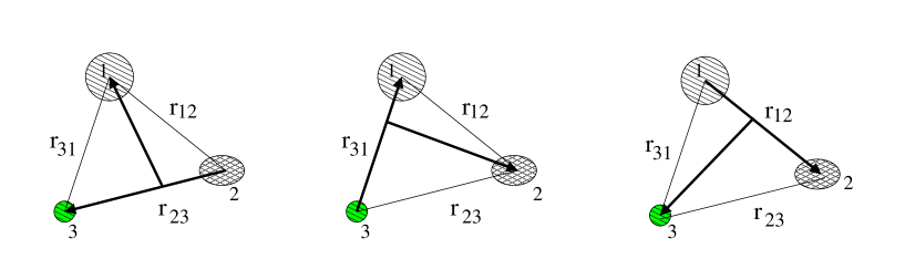
Figure 1: Three sets of Jacobi Coordinates used in the Faddeev Formalism.

The Faddeev equations define three component wave functions $\Psi_{i}^{JM}$, such that the full three-body wavefunction is $\Psi^{JM}=\Psi_{1}^{JM}(x_{1},y_{1})+\Psi_{2}^{JM}(x_{2},y_{2})+\Psi_{3}^{JM}(x_{3},y_{3})$. Here, the components $\Psi_{i}$ are functions of their own ‘natural’ Jacobi coordinate pairs $i$ (as in Fig. 1), and are solutions of the Faddeev coupled equations:

$$(T_{1}+h+V_{1}-E)\Psi_{1}^{JM} = -V_{1}(\Psi_{2}^{JM}+\Psi_{3}^{JM})$$

$$(T_{2}+h+V_{2}-E)\Psi_{2}^{JM} = -V_{2}(\Psi_{3}^{JM}+\Psi_{1}^{JM})$$ (1)

$$(T_{3}+h+V_{3}-E)\Psi_{3}^{JM} = -V_{3}(\Psi_{1}^{JM}+\Psi_{2}^{JM})\;.$$

These equations contain $h=\sum_{i}h_{i}$, the sum of the intrinsic Hamiltonians of each particle $h_{i}$, the relative kinetic energies in each coordinate set $T_{i}=T_{xi}+T_{yi}$ and the two body interactions between the corresponding pair $V_{i}=V_{jk}(r_{jk})$ (both the Coulomb and nuclear interactions). The indexes $i,j,k$ run through (1,2,3) in circular order.

The distances between each pair of particles $\vec{r}_{jk}$, and the distance between the centre of mass of the pair and the corresponding third particle (represented in Fig. (1) by the thin lines), can be expressed in terms of the Jacobian coordinates $(\vec{x}_{i},\vec{y}_{i})$ where $\vec{x}_{i}=\sqrt{A_{jk}}\;\vec{r}_{jk}$ and $\vec{y}_{i}=\sqrt{A_{(jk)i}}\;\vec{r}_{(jk)i}$:

$$\vec{r}_{jk}=\vec{r}_{j}-\vec{r}_{k}\;\;\mbox{~{}and~{}}\vec{r}_{(jk)i}=\vec{r}_{i}-(A_{j}\vec{r}_{j}+A_{k}\vec{r}_{k})/(A_{j}+A_{k})\ .$$ (2)

Note that the reduced masses are defined by $A_{jk}=\frac{A_{j}A_{k}}{A_{j}+A_{k}}$ and $A_{(jk)i}=\frac{(A_{j}+A_{k})A_{i}}{A_{i}+A_{j}+A_{k}}$ with $i,j,k\in(1,2,3)$ where $A_{i}=\frac{m_{i}}{m}$ with $m=1$ a.m.u. and $m_{i}$ the mass of particle $i$ in a.m.u. In FaCE we will use X to refer to the pair ($x_{1},y_{1}$), Y to refer to ($x_{2},y_{2}$) and T to refer to ($x_{3},y_{3}$).

FaCE allows the user to include core excitation of one of the particles. Let us assume one particle $c\in(1,2,3)$ has low lying excited states strongly coupled to the ground state, and which are likely to have important roles in the three body system. Particle c is then treated as the core, and its internal coordinates $\hat{\xi}_{c}$ must be added to the set of Jacobi coordinates to define the full quantum state of the system. The intrinsic Hamiltonian of the core determines a set of eigenstates $\phi_{s_{c}}$ and eigenvalues $\varepsilon_{s_{c}}$,

$$\hat{h}_{c}(\hat{\xi}_{c})\;\phi_{s_{c}}(\hat{\xi}_{c})=\varepsilon_{s_{c}}\;\phi_{s_{c}}(\hat{\xi}_{c})\;\;.$$ (3)

The model then expands the total wavefunction of the system in terms of these $\phi_{s_{c}}$ states, and factorizes the core degrees of freedom from the Jacobi coordinates in each Faddeev component:

$$\Psi_{i}^{JM}(x_{i},y_{i},\hat{\xi}_{c})=\sum_{s_{c}}\;\phi_{s_{c}}(\hat{\xi}_{c})\;\;\psi_{s_{c}}(x_{i},y_{i})\;,$$

with $i=1,2,3$. Here $\psi_{s_{c}}$ contains the radial, angular and spin of the remaining two particles relative to the chosen core. This model is advantageous if only a small number of core states $\phi_{s_{c}}$ is required to describe the system accurately, which is normally true for systems close to the driplines.

FaCE uses the hyperspherical method to convert two-dimensional partial differential equations into a set of coupled one-dimensional equations. The Jacobi coordinates $(x_{i},y_{i})$ are transformed into the hyperspherical coordinates (hyper-radius $\rho_{i}$ and hyper-angle $\theta_{i}$) defined as

$$\rho^{2}=x_{i}^{2}+y_{i}^{2}=\sum_{i}^{3}A_{i}r_{i}^{2}\hskip 14.22636pt\mbox{and}\hskip 14.22636pt\theta_{i}=\arctan(\frac{x_{i}}{y_{i}})\;\;.$$ (4)

The hyper-radius is invariant under translations, rotations and $(i,j)$ permutations, and is directly related to the overall size of the nucleus whereas the hyper-angle contains radial correlations and is related to the relative magnitude of the two Jacobi coordinates. The hyper-radius is the same for all $i$=1,2,3, this being a basic advantage offered by the hyperspherical coordinate system, while the hyper-angle $\theta_{i}=\arctan(\frac{x_{i}}{y_{i}})$ is different for the various X, Y, T bases.

The transformation from a Jacobian coordinate set to a hyperspherical coordinate system does not affect the angular and spin variables, nor the degrees of freedom of the core. Isospin dependence is not explicitly introduced since typically the interactions to be used have a fixed isospin.

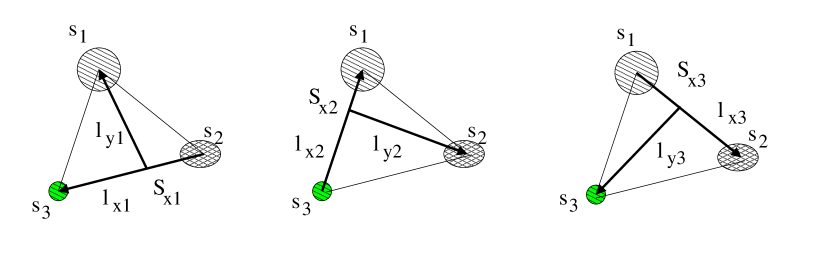
Figure 2: Jacobi coordinates and the notation for the corresponding angular momenta.

For a given Jacobi set $(x_{i},y_{i})$, we need to define and couple together the associated orbital angular momenta $(l_{xi},l_{yi})$, as well as the states and the spins of the three particles $s_{i},s_{j},s_{k}$, as shown in Fig. 2. The core particle will have in FaCE an index for its different excited states, but for the presentation below we assume that the spin value $s_{c}$ suffices to identify its state. A partial wave decomposition for each Faddeev component uses the following the coupling order

$$\Psi_{i}^{JM} = \sum_{l_{xi},l_{yi},L_{i}}\;\;\sum_{s_{j},s_{k},S_{xi}}\;\;\sum_{J_{i},s_{i}}\psi^{i,L_{i}S_{xi}s_{i}J}_{l_{xi}l_{yi}}(x_{i},y_{i})\;\;|i:\{(l_{xi},l_{yi})L_{i},\;(s_{j},s_{k})S_{xi}\}J_{i};s_{i}\rangle^{J}$$

$$\equiv \sum_{\alpha_{i}}\psi^{i,J}_{\alpha_{i}}(x_{i},y_{i})\;\;|i:~{}\alpha_{i}\rangle^{J}$$

with the abbreviation $\alpha_{i}\equiv\{(l_{xi},l_{yi})L_{1},\;(s_{j},s_{k})S_{xi}\}J_{i};s_{i}$ for the quantum numbers of each component $i$. One of the $s_{i},s_{j},s_{k}$ in $\alpha_{i}$ will identify the excitable core state $s_{c}$.

The two-dimension radial wavefunction $\psi^{i,J}_{\alpha_{i}}(x_{i},y_{i})$ is next expanded in the hyperspherical variables. The separation between hyper-angle and hyper-radial dependence of the wavefunction makes use of the fact that the hyper-angle functions, eigensolutions of the hyper-angular (centrifugal) part of the three-body kinetic energy operator delves , are explicitly defined in terms of the Jacobi polynomials:

$$\psi^{i,J}_{\alpha_{i}}(x_{i},y_{i}) = \rho_{i}^{-\frac{5}{2}}\sum_{K_{i}}\;\chi^{i,J}_{\alpha_{i}K_{i}}(\rho)\;\;\varphi_{K_{i}}^{l_{xi}l_{yi}}(\theta_{i})\;\;,$$ (6)

$$\mbox{with}\;\;\;\;\;\varphi_{K_{i}}^{l_{xi}l_{yi}}(\theta_{i}) = N_{K_{i}}^{l_{xi}l_{yi}}\;(\sin\theta)^{l_{xi}}\;(\cos\theta)^{l_{yi}}\;\;P_{n_{i}}^{l_{xi}+1/2,l_{yi}+1/2}(\cos 2\theta_{i})\;\;.$$ (7)

Here $P_{ni}$ is the Jacobi polynomial, $N_{K_{i}}$ is a normalisation coefficient and $K_{i}$ is the hyper-angular-momentum directly related to the order of the corresponding Jacobi polynomial $K_{i}=l_{xi}+l_{yi}+2n_{i}$ ($n_{i}$=0,1,2,…). In order to simplify the notation we will omit whenever possible the total angular momentum and projection labels $JM$ from the wavefunctions.

Introducing this expansion in the Faddeev Equations, and performing the hyper-angular integration, one obtains a set of coupled equations for the wave functions $\chi^{i}_{\alpha_{i}K_{i}}(\rho)$ of Eq. (6)

$$(T_{\rho}+L_{K_{i}}(\rho)-E)\chi^{i}_{\alpha_{i}K_{i}}(\rho)+\sum_{j\alpha_{j}K_{j}}V^{ij}_{\alpha_{i}K_{i},\alpha_{j}K_{j}}(\rho)\chi^{j}_{\alpha_{j}K_{j}}(\rho)=0,$$ (8)

where $T_{\rho}=-\frac{\hbar^{2}}{2m}\frac{d^{2}}{d\rho^{2}}$, and the centrifugal potential is $L_{K_{i}}(\rho)=\hbar^{2}(K_{i}+3/2)(K_{i}+5/2)/(2m\rho^{2})$. The couplings are the hyper-angular integrations of the two-body interaction $V^{ij}_{\alpha_{i}K_{i},\alpha_{j}K_{j}}(\rho)=<\varphi_{K_{j}}^{l_{xj}l_{yj}}(\theta_{j})|\hat{V}_{ij}|\varphi_{K_{i}}^{l_{xi}l_{yi}}(\theta_{i})>$. In FaCE, these hyper-angular integrations are performed using Gauss-Jacobi quadrature on a grid with $N_{jac}$ points (defined in namelist grids in the manual). Gauss-Jacobi quadrature points are evenly spaced in hyper-angle.

In order to solve these coupled equations, the hyper-radial behaviour is expanded in terms of orthonormal basis functions

$$R_{n}(\rho)=\rho^{5/2}\rho_{0}^{-3}[n!/(n+5)!]^{1/2}L_{n}^{5}(z)\exp(-z/2)\ ,$$ (9)

where $z=\rho/\rho_{0}$ with scaling radius $\rho_{0}$ and $L^{\alpha}_{n}(z)$ is an associated Laguerre polynomial, as

$$\chi^{i,J}_{\alpha_{i}K_{i}}(\rho)=\sum_{n=0}^{N_{b}}a^{in,J}_{K_{i}\alpha_{i}}R_{n}(\rho)\;.$$ (10)

The potential matrix element integrals of the $R_{n}(\rho)$ functions are calculated using Gauss-Laguerre quadrature with $N_{lag}$ points, which must be greater than the number $N_{b}$ of basis polynomials. $N_{b}$ is set from the namelist solve, and $N_{lag}$ is set from the namelist grids, while the quadrature points and weights are determined through finding numerically the roots of $L^{5}_{N_{lag}}(z)=0$.

The kinetic energy matrix elements, including the centrifugal barrier, are

$$\langle R_{n}(\rho)|T_{K_{i}}|R_{n^{\prime}}(\rho)\rangle=\frac{\hbar^{2}}{2m}\left[\frac{1}{2}-\frac{\delta_{n{n^{\prime}}}}{4}+\frac{n_{<}}{6}+\frac{K_{i}(K_{i}+4)}{120}\left\{5(n_{>}-n_{<}+1)+n_{>}+n_{<}+1\right\}\right]$$

where $n_{<}=\min(n,{n^{\prime}})$ and $n_{>}=\max(n,{n^{\prime}})$.

After introducing the hyperspherical expansions Eqs. (6,10) into the Faddeev coupled equations Eq. (1), one arrives at a set of simultaneous linear equations

$$H{\bf a}=E{\bf a}$$ (11)

for the coefficients ${\bf a}\equiv\{a\}$. We shall only be calculating bound or pseudo-bound states, for which the wave functions $\chi(\rho)$ vanish at both $\rho=0$ and $\rho\rightarrow\infty$. This is guaranteed by those same properties of the basis functions of Eq. (9).

III The three body matrix elements

The complete wave function solution for a given $J$ (which will henceforth often be omitted) is

$$\Psi=\sum_{i=1}^{3}\sum_{\alpha_{i}}\psi^{i}_{\alpha_{i}}(x_{i},y_{i})\;\;|i:~{}\alpha_{i}\rangle\;,$$ (12)

where there is an implicit sum over hyper-moment K due to the expansion of $\psi^{i}_{\alpha_{i}}(x_{i},y_{i})$ as in Eq. (6). The Hamiltonian matrix will therefore require overlap integrals of the potentials between pairs of the overcomplete basis set $\{|i:\alpha_{i}\rangle\}$. We will need transformation matrices for the rotations $|k:\alpha_{k}\rangle\rightarrow|i:\alpha_{i}\rangle$ clockwise, and $|i:\alpha_{i}\rangle\leftarrow|j:\alpha_{j}\rangle$ anticlockwise, between the three Faddeev components. Considering $(i,j,k)$ the circular order, the expressions that allow the transformation (which conserves total angular moment $L$ and hypermoment $K$) between Faddeev components in both directions are

$$|i:\alpha_{i}\rangle = \sum_{S_{t},S_{xk}}\sum_{L_{k},l_{xk},l_{yk}}\sum_{J_{k}}(-1)^{2(J-S_{xk}-s_{k})+S_{t}+S_{xi}-s_{i}}\times\hat{S_{t}}^{2}\hat{S_{xk}}\hat{S_{xi}}\hat{J_{k}}\hat{J_{i}}\;W(L_{i},S_{xi},J,s_{i};J_{i},S_{t})$$ (13)

$$\times W(s_{k},s_{j},S_{t},s_{i};S_{xi},S_{xk})\;W(s_{k},S_{xk},J,L_{k};S_{t},J_{k})\;RR(l_{xi},l_{yi};l_{xk},l_{yk};L_{k})\delta_{L_{i}L_{k}}|k:\alpha_{k}\rangle\;;$$

$$|i:\alpha_{i}\rangle = \sum_{S_{t},S_{xj}}\sum_{L_{j},l_{xj},l_{yj}}\sum_{J_{j}}(-1)^{2(J-S_{xj}-s_{j})+S_{t}-S_{xj}-s_{j}}\times\hat{S_{t}}^{2}\hat{S_{xj}}\hat{S_{xi}}\hat{J_{j}}\hat{J_{i}}\;W(L_{i},S_{xi},J,s_{i};J_{i},S_{t})$$ (14)

$$\times W(s_{j},s_{k},S_{t},s_{i};S_{xi},S_{xj})\;W(s_{j},S_{xj},J,L_{j};S_{t},J_{j})\;RR(l_{xi},l_{yi};l_{xj},l_{yj};L_{j})\delta_{L_{i}L_{j}}|j:\alpha_{j}\rangle$$

where $RR(l_{xi},l_{yi};l_{xj},l_{yj};L)$ are the Raynal-Revai coefficientsray70 . The two above equations introduce two kinds of norm matrices $N^{ij}$ and $\tilde{N}^{ik}$ such that $|i\rangle=N^{ij}|j\rangle$ and $|i\rangle=\tilde{N}^{ik}|k\rangle$. That is, the matrix elements of $N^{ij}$ are the basis-state overlaps

$$N^{ij}_{\alpha_{i}\alpha_{j}}=\langle j:\alpha_{j}|i:\alpha_{i}\rangle\ ,$$

so that $N^{ij}N^{jk}=\tilde{N}^{ik}$.

There are several kinds of matrix elements needed for the matrix $H$ in the Faddeev equations of Eq. (11). The general potential we are considering is:

$$\hat{V}_{jk}=\hat{V}_{i}(x_{i})=V^{c}_{i}(x_{i})+\hat{SO}\;V^{so}_{i}(x_{i})+\hat{Q}\;V^{Q}_{i}(x_{i})+\hat{T}\;V^{T}_{i}(x_{i})+\hat{SS}\;V^{SS}_{i}(x_{i})\;,$$ (15)

where $V^{c}_{i}$ stands for the central interaction, $\hat{SO}$ and $V^{so}_{k}$ are the spin-orbit operator and the spin-orbit radial form-factor respectively, $\hat{Q}$ and $V^{Q}_{i}(x_{i})$ are the tensor operator and radial shape for the multipoles of the deformed potential, $\hat{T}$ and $V^{T}_{i}(x_{i})$ stand for the standard tensor operator brink and radial dependence for the tensor NN interaction, and finally $\hat{SS}$ and $V^{SS}_{i}$ are the spin-spin operator and the corresponding form-factor. All these are included in FaCE. The parameters for the corresponding radial form factors are defined in namelist poten (see manual for details).

The matrix elements of $\hat{V}_{i}(x_{i})$ are preferentially calculated between basis states of the same $i$ component. The norm matrix elements $N^{ij}$ allow us to express general potential matrix elements in mixed representations, in terms of the preferential Faddeev representation. For example:

$$\langle j:\alpha_{j}^{\prime}\|V_{i}\|i:\alpha_{i}\rangle=\sum_{\alpha_{i}^{\prime}}N^{ij^{\prime}}_{\alpha_{i}^{\prime}\alpha_{j}^{\prime}}\langle i:\alpha_{i}^{\prime}\|V_{i}\ |i:\alpha_{i}\rangle\;,$$ (16)

or, for cases when the potential is most easily presented in one particular Jacobi coordinate set:

$$\langle j^{\prime}:\alpha_{j}^{\prime}\|V_{i}\|j:\alpha_{j}\rangle=\sum_{\alpha_{i}^{\prime}\alpha_{i}}N^{i^{\prime}j^{\prime}}_{\alpha_{i}^{\prime}\alpha_{j}^{\prime}}\langle i:\alpha_{i}^{\prime}\|V_{i}\|i:\alpha_{i}\rangle N^{ji}_{\alpha_{i}\alpha_{j}}\;.$$ (17)

In this section we first consider the angular and spin matrix elements, and these will be later multiplied by numerical integrals over the hyper-angle $\theta_{i}$ to obtain $V^{ij}_{\alpha_{i}K_{i},\alpha_{j}K_{j}}(\rho)$ as in Eq. (8) and the hyper-radius $\rho$ after the expansion in Eq. (10). We will use $W_{ii^{\prime}}$ to denote the matrix elements over the angular momentum basis states. We use:

$$\langle i:{\alpha_{i}^{\prime}}\|V_{i}\|i:\alpha_{i}\rangle=W_{ii^{\prime}}^{c}\;V^{c}_{i}(x_{i})+W_{ii^{\prime}}^{so}\;V^{so}_{i}(x_{i})+W_{ii^{\prime}}^{Q}\;V^{Q}_{i}(x_{i})+W_{ii^{\prime}}^{T}\;V^{T}_{i}(x_{i})+W_{ii^{\prime}}^{SS}V^{SS}_{i}(x_{i})\;.$$ (18)

The potential matrix element for the central part is diagonal in all angular and spin variables. Next, let us consider the spin-orbit part. As all three particles may have spin, we have introduced the general spin operator $\Sigma_{i}\equiv\Gamma_{ij}s_{j}+\Gamma_{ik}s_{k}$, where $\Gamma_{ij}$ and $\Gamma_{ik}$ select which of the spins are to be dynamically coupled, and with which relative strength. The matrix elements for this operator are

$$\langle i\mbox{:}\alpha_{i}^{\prime}\|l_{xi}\cdot\Sigma_{i}\|i\mbox{:}\alpha_{i}\rangle = \delta_{s_{i}^{\prime}s_{i}}\delta_{s_{j}^{\prime}s_{j}}\delta_{s_{k}^{\prime}s_{k}}\delta_{JJ^{\prime}}\delta_{J_{i}^{\prime}J_{i}}\delta_{l_{yi}^{\prime}l_{yi}}\delta_{l_{xi}^{\prime}l_{xi}}(-1)^{2J+3J_{i}^{\prime}+l_{yi}+l_{xi}^{\prime}+2s_{i}+s_{j}+s_{k}}$$ (23)

$$\times \hat{S_{xi}^{\prime}}\hat{S_{xi}}\hat{L_{i}^{\prime}}\hat{L_{i}}\hat{l_{xi}}\sqrt{l_{xi}(l_{xi}+1)}\left\{\begin{array}[]{ccc}L_{i}^{\prime}&l_{i}&1\\ S_{xi}&S_{xi}^{\prime}&J_{i}\end{array}\right\}\left\{\begin{array}[]{ccc}L_{i}^{\prime}&L_{i}&1\\ l_{xi}&l_{xi}^{\prime}&l_{yi}^{\prime}\end{array}\right\}$$

$$\times \left[\Gamma_{ij}(-1)^{S_{xi}}\hat{s_{j}}\sqrt{s_{j}(s_{j}+1)}\left\{\begin{array}[]{ccc}S_{xi}^{\prime}&S_{xi}&1\\ s_{j}&s_{j}^{\prime}&s_{k}^{\prime}\end{array}\right\}+\Gamma_{ik}(-1)^{S_{xi}^{\prime}}\hat{s_{k}}\sqrt{s_{k}(s_{k}+1)}\left\{\begin{array}[]{ccc}S_{xi}^{\prime}&S_{xi}&1\\ s_{k}&s_{k}^{\prime}&s_{j}^{\prime}\end{array}\right\}\right].$$ (28)

Typically the interaction between a deformed excitable nucleus and another particle is expanded in multipoles. The essential angular momentum operator is a tensor interaction of the type $C_{Q}(\hat{l}_{x})\cdot C_{Q}(\hat{s})$. Depending on the Faddeev component and the subscript that specifies the deformed nucleus, all forms of the operator are needed: a) $C_{Q}(\hat{l}_{xi})\cdot C_{Q}(\hat{s}_{i})$, b) $C_{Q}(\hat{l}_{xi})\cdot C_{Q}(\hat{s}_{j})$ and c) $C_{Q}(\hat{l}_{xi})\cdot C_{Q}(\hat{s}_{k})$. We next present the results for these matrix elements:

$$a)\;\;\; \langle i:\alpha_{i}^{\prime}\|C_{Q}(\hat{l}_{xi})\cdot C_{Q}(\hat{s}_{i})\|i:\alpha_{i}\rangle=\delta_{s_{j}^{\prime}s_{j}}\delta_{s_{k}^{\prime}s_{k}}\delta_{JJ^{\prime}}\delta_{l_{yi}^{\prime}l_{yi}}\delta_{S_{xi}^{\prime}S_{xi}}(-1)^{J^{\prime}+2J_{i}+l_{yi}^{\prime}+L_{i}^{\prime}+L_{i}+s_{i}^{\prime}+S_{xi}^{\prime}}\hat{J_{i}^{\prime}}\hat{J_{i}}\hat{L_{i}^{\prime}}\hat{L_{i}}\hat{l_{xi}^{\prime}}\hat{l_{xi}}\hat{s_{i}^{\prime}}$$ (37)

$$\times\left\{\begin{array}[]{ccc}J_{i}^{\prime}&J_{i}&Q\\ s_{i}&s_{i}^{\prime}&J^{\prime}\end{array}\right\}\left\{\begin{array}[]{ccc}J_{i}^{\prime}&J_{i}&Q\\ L_{i}&L_{i}^{\prime}&S_{xi}^{\prime}\end{array}\right\}\left\{\begin{array}[]{ccc}L_{i}^{\prime}&L_{i}&Q\\ l_{xi}&l_{xi}^{\prime}&l_{yi}^{\prime}\end{array}\right\}\left(\begin{array}[]{ccc}l_{xi}^{\prime}&Q&l_{xi}\\ 0&0&0\end{array}\right)\langle s_{i^{\prime}}\|C_{Q}(\hat{s}_{i})\|s_{i}\rangle\;;$$

$$b)\;\;\; \langle i:\alpha_{i}^{\prime}\|C_{Q}(\hat{l}_{xi})\cdot C_{Q}(\hat{s}_{j})\|i:\alpha_{i}\rangle=\delta_{s_{i}^{\prime}s_{i}}\delta_{s_{k}^{\prime}s_{k}}\delta_{JJ^{\prime}}\delta_{J_{i}J_{i}^{\prime}}\delta_{l_{yi}^{\prime}l_{yi}}(-1)^{J^{\prime}+l_{yi}^{\prime}+S_{xi}^{\prime}+S_{xi}+s_{k}^{\prime}+s_{j}^{\prime}}\hat{L_{i}^{\prime}}\hat{L_{i}}\hat{S_{xi}^{\prime}}\hat{S_{xi}}\hat{l_{xi}^{\prime}}\hat{l_{xi}}\hat{s_{j}^{\prime}}$$ (46)

$$\times\left\{\begin{array}[]{ccc}L_{i}^{\prime}&L_{i}&Q\\ S_{xi}&S_{xi}^{\prime}&J_{i}^{\prime}\end{array}\right\}\left\{\begin{array}[]{ccc}L_{i}^{\prime}&L_{i}&Q\\ l_{xi}&l_{xi}^{\prime}&l_{yi}^{\prime}\end{array}\right\}\left\{\begin{array}[]{ccc}S_{xi}^{\prime}&S_{xi}&Q\\ s_{j}&s_{j}^{\prime}&s_{k}\end{array}\right\}\left(\begin{array}[]{ccc}l_{xi}^{\prime}&Q&l_{xi}\\ 0&0&0\end{array}\right)\langle s_{j^{\prime}}\|C_{Q}(\hat{s}_{j})\|s_{j}\rangle\;;$$

$$c)\;\;\; \langle i:\alpha_{i}^{\prime}\|C_{Q}(\hat{l}_{xi})\cdot C_{Q}(\hat{s}_{k})\|i:\alpha_{i}\rangle=\delta_{s_{i}^{\prime}s_{i}}\delta_{s_{j}^{\prime}s_{j}}\delta_{JJ^{\prime}}\delta_{J_{i}J_{i}^{\prime}}\delta_{l_{yi}^{\prime}l_{yi}}(-1)^{J^{\prime}+l_{yi}^{\prime}+2S_{xi}^{\prime}+s_{k}+s_{j}^{\prime}}\hat{L_{i}^{\prime}}\hat{L_{i}}\hat{S_{xi}^{\prime}}\hat{S_{xi}}\hat{l_{xi}^{\prime}}\hat{l_{xi}}\hat{s_{k}^{\prime}}$$ (55)

$$\times\left\{\begin{array}[]{ccc}L_{i}^{\prime}&L_{i}&Q\\ S_{xi}&S_{xi}^{\prime}&J_{i}^{\prime}\end{array}\right\}\left\{\begin{array}[]{ccc}L_{i}^{\prime}&L_{i}&Q\\ l_{xi}&l_{xi}^{\prime}&l_{yi}^{\prime}\end{array}\right\}\left\{\begin{array}[]{ccc}S_{xi}^{\prime}&S_{xi}&Q\\ s_{k}&s_{k}^{\prime}&s_{j}^{\prime}\end{array}\right\}\left(\begin{array}[]{ccc}l_{xi}^{\prime}&Q&l_{xi}\\ 0&0&0\end{array}\right)\langle s_{k^{\prime}}\|C_{Q}(\hat{s}_{k})\|s_{k}\rangle\;.$$

The matrix elements between different core states $\langle s_{i^{\prime}}\|C_{Q}(\hat{s}_{i})\|s_{i}\rangle$ depends on the model used. Under the assumption of a pure rotational model, these matrix elements are given by:

$$\langle s_{i^{\prime}}\|C_{Q}(\hat{s}_{i})\|s_{i}\rangle=(-1)^{K-s_{i}^{\prime}}\hat{s_{i}}\left(\begin{array}[]{ccc}s_{i}^{\prime}&Q&s_{i}\\ -K^{\prime}&0&K\end{array}\right)\;,$$ (56)

where $K$ is the quantum number for the rotational band. If the interaction is $\ell-$dependent there is an ambiguity on the choice of the radial form factor (which is defined at the multipole expansion of the deformed potential). The parameter $lpot$ (see manual) controls this choice.

When considering the spin-spin interactions again there are three possibilities depending on the Faddeev components: a) $\langle s_{i}^{\prime}\|\vec{s}_{i}\cdot\vec{s}_{j}\|s_{i}\rangle$; b) $\langle s_{i}^{\prime}\|\vec{s}_{i}\cdot\vec{s}_{k}\|s_{i}\rangle$ and c) $\langle s_{i}^{\prime}\|\vec{s}_{j}\cdot\vec{s}_{k}\|s_{i}\rangle$. After some algebra one can arrive at:

$$a)\;\;\;\langle i:\alpha_{i}^{\prime}\|\hat{s}_{i}\cdot\hat{s}_{j}\|i:\alpha_{i}\rangle = \delta_{s_{i}^{\prime}s_{i}}\delta_{s_{j}^{\prime}s_{j}}\delta_{s_{k}^{\prime}s_{k}}\delta_{JJ^{\prime}}\delta_{L_{i}^{\prime}L_{i}}(-1)^{3J+J_{i}^{\prime}-J_{i}+L_{i}^{\prime}+2S_{xi}-s_{i}+s_{j}+s_{k}}\hat{J_{i}^{\prime}}\hat{J_{i}}\hat{S_{xi}^{\prime}}\hat{S_{xi}}\hat{s_{i}}\hat{s_{j}}$$ (63)

$$\times \sqrt{s_{i}(s_{i}+1)}\sqrt{s_{j}(s_{j}+1)}\left\{\begin{array}[]{ccc}J_{i}^{\prime}&J_{i}&1\\ S_{xi}&S_{xi}^{\prime}&L_{i}^{\prime}\end{array}\right\}\left\{\begin{array}[]{ccc}S_{xi}^{\prime}&S_{xi}&1\\ s_{j}&s_{j}^{\prime}&s_{k}^{\prime}\end{array}\right\}\left\{\begin{array}[]{ccc}s_{i}^{\prime}&s_{i}&1\\ J_{i}&J_{i}^{\prime}&J^{\prime}\end{array}\right\}\;;$$

$$b)\;\;\;\langle i:\alpha_{i}^{\prime}\|\hat{s}_{i}\cdot\hat{s}_{k}\|i:\alpha_{i}\rangle = \delta_{s_{i}^{\prime}s_{i}}\delta_{s_{j}^{\prime}s_{j}}\delta_{s_{k}^{\prime}s_{k}}\delta_{JJ^{\prime}}\delta_{L_{i}^{\prime}L_{i}}(-1)^{3J+J_{i}^{\prime}-J_{i}+L_{i}^{\prime}+S_{xi}+S_{xi}^{\prime}-s_{i}^{\prime}+s_{j}^{\prime}+s_{k}}\hat{J_{i}^{\prime}}\hat{J_{i}}\hat{S_{xi}^{\prime}}\hat{S_{xi}}\hat{s_{i}}\hat{s_{k}}$$ (70)

$$\times \sqrt{s_{i}(s_{i}+1)}\sqrt{s_{k}(s_{k}+1)}\left\{\begin{array}[]{ccc}J_{i}^{\prime}&J_{i}&1\\ S_{xi}&S_{xi}^{\prime}&L_{i}^{\prime}\end{array}\right\}\left\{\begin{array}[]{ccc}S_{xi}^{\prime}&S_{xi}&1\\ s_{k}&s_{k}^{\prime}&s_{j}^{\prime}\end{array}\right\}\left\{\begin{array}[]{ccc}s_{i}^{\prime}&s_{i}&1\\ J_{i}&J_{i}^{\prime}&J^{\prime}\end{array}\right\}\;;$$

$$c)\;\;\;\langle i:\alpha_{i}^{\prime}\|\hat{s}_{j}\cdot\hat{s}_{k}\|i:\alpha_{i}\rangle = \delta_{s_{i}^{\prime}s_{i}}\delta_{s_{j}^{\prime}s_{j}}\delta_{s_{k}^{\prime}s_{k}}\delta_{JJ^{\prime}}\delta_{J_{i}^{\prime}J_{i}}\delta_{S_{xi}S_{xi}^{\prime}}\delta_{L_{i}^{\prime}L_{i}}(-1)^{S_{xi}+s_{j}+s_{k}}\hat{s_{j}}\hat{s_{k}}$$ (73)

$$\times \sqrt{s_{j}(s_{j}+1)}\sqrt{s_{k}(s_{k}+1)}\left\{\begin{array}[]{ccc}s_{j}^{\prime}&s_{j}&1\\ s_{k}&s_{k}^{\prime}&S_{xi}^{\prime}\end{array}\right\}\;.$$

A realistic NN force contains a tensor interaction of the type $T_{2}(s_{j}s_{k})\cdot C_{2}(l_{xi})$ which also needs to be considered. Below is the expression for these matrix elements after working out the algebra:

$$\langle i:\alpha_{i}^{\prime}\|T_{2}(s_{j}s_{k})\cdot C_{2}(l_{xi}\|i:\alpha_{i}\rangle = \delta_{s_{i}^{\prime}s_{i}}\delta_{s_{j}^{\prime}s_{j}}\delta_{s_{k}^{\prime}s_{k}}\delta_{JJ^{\prime}}\delta_{J_{i}^{\prime}J_{i}}\delta_{l_{yi}^{\prime}l_{yi}}(-1)^{3J_{i}+l_{yi}-S_{xi}^{\prime}}\hat{2}\hat{S_{xi}^{\prime}}\hat{S_{xi}}\hat{L_{i}^{\prime}}\hat{L_{i}}\hat{l_{xi}}\hat{l_{xi}^{\prime}}\hat{s_{j}^{\prime}}\hat{s_{k}^{\prime}}\sqrt{s_{j}(s_{j}+1)}$$ (83)

$$\times \sqrt{s_{k}(s_{k}+1)}\left\{\begin{array}[]{ccc}S_{xi}^{\prime}&S_{xi}&2\\ L_{i}&L_{i}^{\prime}&J_{i}^{\prime}\end{array}\right\}\left\{\begin{array}[]{ccc}L_{i}^{\prime}&L_{i}&2\\ l_{xi}&l_{xi}^{\prime}&l_{yi}^{\prime}\end{array}\right\}\left(\begin{array}[]{ccc}l_{xi}^{\prime}&2&l_{xi}\\ 0&0&0\end{array}\right)\left\{\begin{array}[]{ccc}S_{xi}^{\prime}&S_{xi}&2\\ s_{j}^{\prime}&s_{j}&1\\ s_{k}^{\prime}&s_{k}&1\\ \end{array}\right\}.$$

Few-body models often include effective three-body potentials to describe the influence of dynamics not explicitly described by two-body potentials. We have parameterised the simplest diagonal form of such a potential:

$$\langle i^{\prime}:\alpha_{i}^{\prime}\|\hat{V}_{3}\|i:\alpha_{i}\rangle=\delta_{i^{\prime}i}\delta_{\alpha_{i}^{\prime}\alpha_{i}}V_{3}(\rho)\ .$$ (84)

IV Pauli Blocking

Often within a three-body calculation, it is necessary to eliminate the Pauli forbidden two-body bound states before diagonalisation. This may be accomplished by several methods dan98 ; thom00 : by projection operators inserted in three-body Hamiltonian before diagonalisation, or by transforming the two-body potentials in those partial wave channels with deeply-bound forbidden states in a way that preserves phase (spectral) equivalence. We here adopt this second approach, and use supersymmetric transformations of the two-body potentials in order to eliminate a required set of bound states. All the parameters relative to the method are specified in the namelist b2states and the specific characteristics of the two-body bound states to be calculated are defined in b2state (see manual for details).

Sometimes, it is useful to calculate the two body state generated by a given effective interaction, or explore how to adjust the two body interaction to obtain a given binding energy. FaCE allows you to calculate bound states without feeding them into the SUSY transformation subroutine (see b2states in the manual for details).

IV.1 Elimination of Two-body bound states

A supersymmetric transformation of the set of potentials ss enables the removal of an arbitrary bound state, while keeping the spectral ($S$-matrix) equivalence of the initial and the transformed Hamiltonians. In partition $k$, and in each two-body spin-parity channel, the initial Hamiltonian $\hat{H}_{0}$ for the interaction of bodies $i,j$ couples $N$ two-body channels for total angular momentum $j_{k}$. The two-body equation is then

$$\Bigl{(}-\frac{\hbar^{2}}{2\mu_{ij}}\Bigl{[}\frac{d^{2}}{dr^{2}}+\frac{{\ell_{n}}({\ell_{n}}+1)}{r^{2}}\Bigr{]}-E\Bigr{)}\phi_{n}(r)+\sum_{n^{\prime}}^{N}V_{nn^{\prime}}(r)~{}\phi_{n^{\prime}}(r)=0\ ,$$ (85)

where $n$ is a channel index set $\{l_{x_{k}},(s_{i},s_{j})S_{x_{k}};j_{k}\}$, $r\equiv r_{ij}$, $\ell_{n}\equiv l_{x_{k}(n)}$, and $\mu_{ij}$ is the reduced mass for bodies $i,j$. The threshold energies $\epsilon_{n}=\varepsilon_{s_{i}}+\varepsilon_{s_{j}}$ are included in the diagonal matrix elements $V_{nn}(r)$, in addition to the couplings defined by Eq. (15). We start with the real symmetric potential matrix $\hat{V}_{0}(r)=\{V_{n^{\prime}n}(r)\}$ at each radius, and repeat the following supersymmetric transformation for each bound state $p=1$ up to the number of forbidden states $P$.

Let the column vector $\Phi_{p-1}^{\lambda}(r)=\{\phi_{n}^{\lambda}(r)\}$ be the normalised ground state eigensolution of $H_{p-1}$ at real energy $E_{\lambda}$ below all thresholds. By applying a double supersymmetric transformation to $H_{p-1}$ we obtain a new Hamiltonian $H_{p}$ where the potential matrix $\hat{V}_{p-1}(r)$ is replaced by $\hat{V}_{p}(r)$

$$\hat{V}_{p}(r)=\hat{V}_{p-1}(r)-\frac{\hbar^{2}}{\mu_{ij}}\frac{d}{dr}\frac{\Phi_{p-1}^{\lambda}(r)\Phi_{p-1}^{\lambda{\dagger}}(r)}{\int_{0}^{r}\Phi_{p-1}^{\lambda{\dagger}}(t)\Phi_{p-1}^{\lambda}(t)dt}$$ (86)

In the case of vanishing coupling between the channels near the origin, it is possible to deduce the behaviour of the diagonal parts of $\hat{V}_{p}(r)$ at small $r$. If the diagonal matrix of angular moments $\{\ell_{n}\}$ has only one lowest element, say $\ell_{1}$, such that $\ell_{1}<\ell_{n}$ for $n=2,3,...N$, in this channel (index 1) the additional term in the supersymmetric transformed potential $\hat{V}_{p}(r)$ will have a singularity $\hbar^{2}(2\ell_{1}+3)/(2\mu_{ij}r^{2})$ at small $r$, which added to the centrifugal term $\hbar^{2}\ell_{1}(\ell_{1}+1)/(2\mu_{ij}r^{2})$ gives a new centrifugal term $\hbar^{2}(\ell_{1}+2)(\ell_{1}+3)/(2\mu_{ij}r^{2})$. The supersymmetric transformation Eq. (86) in this case adds a repulsive core at the origin, by increasing the orbital moment $\ell_{1}$ by 2 units. In all other channels the orbital moments $\ell_{n}$ are not changed. Physically, this corresponds to the conservation of the oscillator quanta $\Lambda=2n_{r}+\ell$ in the system: when reducing the radial quantum number $n_{r}$ by one unit (removing one level) we increase the orbital part $\ell$ by two (for the one channel case we satisfy the Levinson’s theorem). If the diagonal matrix of angular momenta $\{\ell_{n}\}$ has several lowest equal elements, the increase of singularity is shared between these channels, including their coupling potentials.

In FaCE, if supersymmetric transformations are used for any partition $k$, then the transformations up to $\hat{V}_{P}(r)$ must be recalculated for all desired two-body channels $j_{k}$ (all jv in namelist b2state).

V Solving the Faddeev equations

The Faddeev equations Eq. (1) are solved, after expanding on the hyper-angular Eq. (7) and hyper-radial Eq. (9) basis functions, to find square-integrable solutions Eq. (12) for eigenenergies $E$ and eigenvectors ${\bf a}$. For $E<0$ these are bound states, whereas for $E>0$ the eigen-solutions are ‘quasi-bound’ states that form a discrete representation of the continuum. These quasi-bound wave functions may be used, for example in crespo , in the calculations of breakup as inelastic excitations.

The physical normalisation of the wave functions Eq. (12) is $\langle\Psi|\Psi\rangle=1$. If $N$ is the whole normalisation matrix $N^{ij}_{\alpha_{i}\alpha_{j}}$, the eigenvectors ${\bf a}$ are physically normalised when ${\bf a}^{T}N{\bf a}=1$. Note that some eigenvectors will be found that are non-physical, having ${\bf a}^{T}N{\bf a}=0$; in these there is a cancellation between different Faddeev components, and they must be omitted in all bound or breakup state analyses.

V.1 Hamiltonian Reduction procedures

The complete set Eq. (1) of Faddeev equations may be reduced in a number of circumstances. FaCE has the option of ‘isospin’ and ‘orthonormal’ reductions, which exactly reproduce a physically chosen subset of the eigen-solutions, and also ‘Feshbach’ reduction, which is a method for approximating the effects of high $K$ partial waves on the solutions. The choice of the reduction method is made through eqn in the input namelist solve (see manual).

V.1.1 Isospin Reduction

Suppose bodies $j$ and $k$ are fermions which are isospin states $T_{z}$ of some particle of isospin $T_{jk}$, with $s_{j}=s_{k}$ half-integral. The requirement of antisymmetrisation under exchange of these bodies is easily satisfied if the partial wave set $\alpha_{i}$ only includes those quantum number sets for which $l_{xi}+S_{xi}+T_{jk}$ is odd. In this way, wave function components that are symmetric under interchange of $j$ and $k$ are eliminated from the basis set for this Faddeev component.

Furthermore, the remaining Faddeev components $\Psi_{j}$ and $\Psi_{k}$ are isospin mirrors of each other. Just one of these wave functions needs to be included explicitly in the equation set to be found numerically, since

$$\Psi_{j}=-(-1)^{T_{jk}}P_{jk}\Psi_{k}$$ (87)

where $P_{jk}$ is the operator permuting the coordinates of particles $j$ and $k$.

The coupled equations

$${\left(\begin{array}[]{ccc}T_{i}+h+V_{i}-E&V_{i}&V_{i}\\ V_{j}&T_{j}+h+V_{j}-E&V_{j}\\ V_{k}&V_{k}&T_{k}+h+V_{k}-E\end{array}\right)}{\left(\begin{array}[]{c}\Psi_{i}\\ \Psi_{j}\\ \Psi_{k}\end{array}\right)}=0$$ (88)

are now reduced to

$${\left(\begin{array}[]{ccc}T_{i}+h+V_{i}-E&V_{i}+V_{i}P_{jk}\\ V_{k}&T_{k}+h+V_{k}+V_{k}P_{jk}-E\end{array}\right)}{\left(\begin{array}[]{c}\Psi_{i}\\ \Psi_{k}\end{array}\right)}=0\ .$$ (89)

The permutation matrix elements are $P_{jk}=(-1)^{(l_{xj}+S_{xj}-s_{2j}-s_{3j})}$.

V.1.2 Orthonormal Reduction

Since basis states $|i:~{}\alpha_{i}\rangle$ in Eq. (12) form an over-complete set, the same set of physical eigen-solutions may be found by transforming the basis set into an orthonormal one.

A rotation matrix $C$ may be found, for example by Gramm-Schmidt orthonormalisation, such that $C^{T}NC=I$, so that the columns of $C$ are vectors that are physically orthonormalised by the norm matrix $N$. This same rotation may be used to transform the Hamiltonian matrix of Eq. (11). Defining $D=C^{-1}=C^{T}N$, then

$$DHC{\bf a}\equiv H^{\prime}{\bf a}^{\prime}=E{\bf a}^{\prime}$$

is an orthogonal transformation of the original eigenvalue problem, with the same eigenvalues. The original eigensolutions may be regained as ${\bf a}^{\prime}=C{\bf a}$. The new matrix $H^{\prime}$ is real and symmetric; this proves that the eigenvalues of Eq. (11) are real even though $H$ is not symmetric.

V.1.3 Feshbach Reduction

Another reduction method, also called the semi-adiabatic reduction method, constructs an effective coupling matrix at each $\rho$ value using Feshbach’s expression feshbach for effective interactions in a subspace.

Consider the set of $N$ coupled equations for the wave functions $\chi^{i}_{\alpha_{i}K_{i}}$ as in Eq. (8). Take the subset of the equations of this system with largest $K_{i}$ and core excitation energy $\varepsilon_{s_{c}}$. In these channels, an adiabatic condition might be fulfilled, where the hyper-radial kinetic energy $T_{\rho}$ is small and can be neglected. Thus we have an option of keeping this kinetic energy term in only the subset of channels $i=1,\cdots,M$, and of neglecting $T_{\rho}$ for $i=M+1,\cdots,N$. For each $\rho$ value, let us rewrite the system Eq. (8) in the following matrix form:

$$\left(\begin{array}[]{cccccccccc}{\bf A}-E&{\bf B}\\ {\bf C}&{\bf D}-E\end{array}\right)\left(\begin{array}[]{c}{\bf\chi^{(a)}}\\ {\bf\chi^{(b)}}\end{array}\right)=0,$$ (94)

where ${\bf A}$ contains the exact $T_{\rho}+L_{K_{i}}(\rho)$ terms, but ${\bf D}$ contains only the $L_{K_{i}}(\rho)$ terms. The ${\bf B}$ and ${\bf C}$ are the block off-diagonal matrices. The solution vectors are ${\bf\chi^{(a)}}=(\chi_{1}\cdots\chi_{M})$ and ${\bf\chi^{(b)}}=(\chi_{M+1}\cdots\chi_{N})$.

Solving the matrix Eq. (94) formally we obtain:

$$\chi^{(b)}=({\bf D}-E)^{-1}{\bf C}\chi^{(a)},$$ (95)

and substituting Eq. (95) into our system Eq. (94) we get a reduced subset of coupled equations for $\chi^{(a)}$

$$\left({\bf A}-E+{\bf B}({\bf D}-E)^{-1}{\bf C}\right)\chi^{(a)}=0.$$ (96)

¿From Eq. (96), we see that the reduction of the coupled equations from $N\times N$ to a smaller $M\times M$ set consists in adding a ‘Feshbach’ term ${\bf B}({\bf D}-E)^{-1}{\bf C}$ to the effective interaction in the retained subspace.

Strictly speaking, the Feshbach term should be recalculated for every eigen-energy $E$, but in practice we calculate the Feshbach term once for the fixed ‘Feshbach energy’ $E=E_{F}$, which should be chosen near the eigen-energy of the state of most interest, such as the ground state energy. Variables efesh and kmaxf in the input namelist solve are the Feshbach energy and the K-value above which the Feshbach approximation is introduced (see manual).

V.2 Diagonalisation procedure

The subroutine fadco in FaCE evaluates all the potential matrix elements as functions of $\rho$. After the above possible reductions, the Hamiltonian matrix appearing in the Faddeev Equations Eq. (11) is determined by hyper-radial integrals using the radial basis function Eq. (9).

For the general eigenvalue solution of Eq. (11), where $H$ is a real matrix not necessarily symmetric, we use the subroutine F02AGF from the Nag library, which proceeds via reduction to Hessenberg form, to find all eigensolutions.

If only selected eigenvalues are required, and the input parameter meigs (introduced in solve) is non-zero and less than the dimension of the $H$ matrix of Eq. (11), a more efficient method is that of inverse iteration. Starting from some energy $E_{0}$, and some initial guess ${\bf a}^{(0)}$ for an eigenvector, the solution of the simultaneous linear equations $(H-E_{0}){\bf a}^{(n)}={\bf a}^{(n-1)}$ for $n\geq 1$ will converge to the eigensolution with energy nearest $E_{0}$. This method is effective for $E_{0}$ less than the ground state energy, when there are no nearly-degenerate eigenvalues. It may be generalised to finding the several eigenvalues nearest $E_{0}$ by orthogonalising ${\bf a}^{(n)}$ at each iteration to the set of eigenvectors already found.

VI Computer programme and Input manual

Given the description covered in the previous sections, the FaCE manual is presented as a sequence of namelists with explanatory names for the variables. Nevertheless it is useful to remind the user that the parameters delimiting the three body space are: the number of Laguerre polynomials $N_{b}$ for the hyper-radial part, together with the Jacobi polynomials for the hyper-angular part $N_{jac}$; the maximum angular momentum that are to be taken into account in each Faddeev partition $l_{xmax}(i),l_{ymax}(i)$, and the number of $K$-harmonics $K_{max}(l,i)$.

The source code is distributed with separate makefiles for Sun f90 compilers (standing alone, or with system Sun Performance Library and Nag libraries) and for Linux, where there are Intel ifort and Portland Group pgf90 makefiles, the latter optionally with system Lapack and Blas libraries. The suitable one of these makefiles should be renamed to ‘makefile’.

FaCE uses F02AGF, M01DAF and M01ZAF routines from the Nag library, and DGETRF, DGETRS and DGEMM from the Blas library. The original source codes for the Nag and Blas subroutines are contained in the package for compilation where not otherwise available.

VI.1 Input namelists

• &fname
  nfile[A*20], desc[A*80]
  nfile is the root name of the output files and desc is a heading that should describe and identify the run.

• &scale
  amn, hc [r*8]
  amn is the mass of the nucleon and hc is the planck constant multiplied by the velocity of light in [MeV fm].

• &nuclei
  name(1:3)[A*8], mass(1:3), z(1:3), radius(1:3)[r*8]
  Each of the three interacting nuclei are characterised by their name, mass, charge and radius.

• &identical
  id(1:3)[logical], iso(1:3)[r*8]
  If id(j) is true then the interacting pair in partition j are 2 identical particles. This variable affects the choice of the basis: if particles are identical, an isospin reduction is performed. iso contains the isospin of the interacting pair to be used when $id(j)$ is true, to omit non-antisymmetric partial waves in that partition.

• &total
  ngt[int], gtot(1:ngt)[r*8], gparity(1:ngt)[int]
  ngt $\rightarrow$ the number of states to be calculated, gtot and gparity hold their total spin and parity(even$=+1$, odd$=-1$) respectively.

• &particles
  ns(1:3)[int], spin(1:ns,1:3)[r*8], parity(1:ns,1:3)[int], energy(1:ns,1:3)[r*8]
  This namelist defines intrinsic properties of the three bodies. For each of the 3 nuclei: ns(j) specifies the number of states to be included for nucleus j. For each of its ns(j) states, one should specify the spin, parity(+1/-1) and its energy relative to the energy of the ground state of that nucleus j.

• &em
  corek(1:3), def(2:mmultipoles,1:3)[r*8]

  This namelist contains the electromagnetic information on each of the three bodies.
  corek(j) $\rightarrow$ projection of the spin of nucleus $j$ in its rest frame
  def(q,j) $\rightarrow$ deformation length in the $q$ multipole of nucleus $j$.

• &waves
  This namelist contains the definition of the channels per partition.

  sym(3)[A*1] the name (e.g ’T’, ’X’ or ’Y’) of each partition.

  auto(3)[logical] $\rightarrow$ if ‘T’ then FACE generates automatically the channels allowed given maximum quantum numbers for each Faddeev partition. Otherwise, quantum numbers for $nc(j)$ channels are explicitly read in.

  If auto is false:
  nc(3)[int] $\rightarrow$ number of channels per partition (less than $mfchan$).
  lx(mfchan,3)[int], ly(mfchan,3)[int], lt(mfchan,3)[int], sx(mfchan,3)[r*8], jp(mfchan,3)[r*8] $\rightarrow$ determine the quantum numbers associated with all channels for each partition in the following coupling order $|[(l_{x},l_{y})l_{t},(s_{i},s_{j})s_{x}]J_{p},icy\rangle$
  icy(mfchan,3)[int],icx1(mfchan,3)[int],icx2(mfchan,3)[int] $\rightarrow$ the state of the spectator, the first and the second interacting particle for the given channel in each partition. The spin of a given state of each of the bodies was defined in particles.
  np(mfchan,3)[int] $\rightarrow$ the number of $K$-harmonics.

  If auto is true:
  lxmax(1:3)[int], lymax(1:3)[int], ltmax(1:3)[int], sxmax(1:3)[r*8], jabmax(1:3)[r*8],
  kmaxa(1:3)[int], kmax(0:maxl,1:3)[int] $\rightarrow$ these establish the maximum quantum numbers allowed in each partition. $kmaxa$ is the $K$ limit for all partial waves, and may be overridden by particular $kmax$ specified.

• &poten
  This namelist defines the radial behaviour of the potentials for each interacting pair.

  detail(3)[A*80] $\rightarrow$ information on the interaction between the interacting pair in that partition
  typc(3)[A*3], pa(6,3),ps(6,3),pp(6,3),pd(6,3),pf(6,3)[r*8] $\rightarrow$ central interaction
  typso(3)[A*3],pso(6,3),psop(6,3),psod(6,3),psof(6,3)[r*8] $\rightarrow$ spin-orbit interaction
  typss(3)[A*3],pss(6,3),psss(6,3),pssp(6,3),pssd(6,3),pssf(6,3) $\rightarrow$ spin-spin interaction
  typt(6,3)[A*3], pt(6,3)[r*8] $\rightarrow$ tensor interaction
  rcoul(3)[r*8],acoul(3)[r*8] $\rightarrow$ the Coulomb interaction
  lpot(3)[int] $\rightarrow$ is useful for $l-$dependent interactions where there is an ambiguity on the radial form factor that should be used for off diagonal couplings. If $lpot=0$, the radial form factor corresponding to the minimum $l_{i},l_{f}$ is used; $lpot=1$, the average is taken; $lpot=2$ the maximum is used; and lpot=3 the final $l_{f}$ (corresponding to the left hand side of the matrix element) is used. Finally, when $lpot\geq 10$, the radial form factor for off-diagonal coupling is determined by $l=lpot-10$, throughout the whole calculation, leaving the monopole terms untouched.
  

  The form factor for the potentials between the interacting pair in each partition is specified by type (gau, ws, rnp, rnn, nul) and the potential parameters for each partial wave (s,p,d,f and a or no extra letter for all). If the type is gau then the interaction is the sum of 3 Gaussians:

  $$V_{gau}^{i}(r)=\sum_{k=1,3,5}pa(k,i)\exp\left[-\left(\frac{r}{pa(k+1,i)}\right)^{2}\right]$$

  If type is ws then the interaction is the sum of 2 Woods-Saxon:

  $$V_{ws}^{i}(r)=\sum_{k=1,4}pa(k,i)\left[1+\exp\left(\frac{r-pa(k+1,i)}{pa(k+2,i)}\right)\right]^{-1}$$

  For the spin-orbit interaction, if type is ’ws’ then the form factor is given by the derivative of two Woods-Saxon:

  $$V_{ws}^{i}(r)=\sum_{k=1,4}\frac{pso(k,i)}{r\;pso(k+2,i)}\frac{\exp(\frac{r-pso(k+1,i)}{pso(k+2,i)})}{[1+\exp(\frac{r-pso(k+1,i)}{pso(k+2,i)})]^{2}}$$

  The Coulomb interaction for the interacting pair in partition (i) is that of a uniform sphere with radius rcoul(i) and diffuseness acoul(i), screened at radius rscreen with a Fermi function of diffuseness ascreen.

  The operator for the tensor force is $12\hat{S}_{12}$ as defined by Brink and Satchler brink . The operator for the spin-spin force is the dot product of the spins of the interacting pair $\vec{s}_{j}\cdot\vec{s}_{k}$. The operator for the spin-orbit is defined in gamso. If the deformation of one of the interacting particles in non zero then higher order multipoles will be automatically added to the monopole interaction based on a spherical harmonic decomposition of a deformed field.

• &pot3b
  typ3b,s3b(ngt),r3b(ngt),a3b(ngt),gtvary $\rightarrow$ specifies the parameters for the diagonal 3-body potential $V_{3}(\rho)$ if typ3b $\neq$ nul. If gtvary, then $ijt=1$ below, otherwise $ijt$ is the $J^{\pi}$ index 1 … $ngt$. If $typ3b={\tt gau}$, then

  $$V_{3}(\rho)=s3b(ijt)\exp\left[-\left(\frac{\rho}{r3b(ijt)}\right)^{2}\right]$$

  If $typ3b={\tt ws}$, then

  $$V_{3}(\rho)=s3b(ijt)\left[1+\exp\left(\frac{\rho-r3b(ijt)}{a3b(ijt)}\right)\right]^{-1}$$

• &gamso
  gamso1, gamso2 $\rightarrow$ the spin-orbit matrix elements are calculated using the following operator $\Gamma_{1}\vec{l}_{x}\cdot\vec{s}_{1}+\Gamma_{2}\vec{l}_{x}\cdot\vec{s}_{2}$ for each partition
  

• &grids
  rr [r*8], nlag,njac [int]
  This section contains radii for the expansions used.
  rr $\rightarrow$ scaling parameter $\rho_{0}$ for the Laguerre basis
  nlag $\rightarrow$ number of Laguerre quadrature points for the $\rho$ coordinate.
  njac $\rightarrow$ number of Jacobi polynomials
  

• &trace
  pripot,vadia [logical]
  Printing options: $pripot$ prints the potential matrix elements, $vadia$ prints the diagonalised coupling eigenvalues (energy surfaces). All of these are printed in the output file with extension lis.

• &b2states
  n2states[int], dx,xmax, [r*8], ipc,lmax,nk [int], rnode,de [r*8],
  Find n2states two-body states in the two-body potentials. Use radial grid 0 to xmax with steps dx. The ipc, lmax, nk and rnode, de are default values for each b2state namelist below.

• &b2state (repeated n2states times)
  pair,kind [int], de [r*8] ipc [int], test [logical], n,nvchan,l,lmax [int],s,jv,rnode [r*8], search,rescale [logical], eigen,potential, fermi [r*8], nomit [int],omit_l1:nomit [int] ,omit_s1:nomit,omit_j1:nomit [r*8], omit_c11:nomit,omit_c21:nomit [int],
  Find two-body eigenstate in the potential pair, of kind=‘occup’ to be used for pauli blocking via the susy transformation; kind=‘transfer’ if one needs to check the properties of a particular two body state, or kind=‘pot’ if one needs to calculate numerically the potential for a particular two body partial wave set, without excluding it. This last option is needed, because whenever there are any occupied states, the potentials for all partial waves sets in that partition need to be calculated numerically.
  ipc = trace level, test=T to ignore this state after finding it.
  Wave functions will have n nodes in channel $\ell$=l up to radius rnode, from a set of $\ell\leq$lmax using coupling order $|\ell,(s_{1}s_{2})s;jv\rangle$. The eigenenergy is eigen in monopole potential multiplied by potential, where search=‘E’ or ‘V’ to search for energy or potential factor respectively. Energies eigen are negative for bound states. Only bound states can be found when search =’E’. Use nomit$>$0 to specifically omit some partial waves from the coupled channels set.
  fermi $<$0, to exclude bound states up to that valence energy,
  fermi $>$0, to exclude the nint(fermi) number of lowest-energy bound states.
  

• &solve
  eig, eimin,eimax,efesh [r*8], eqn[A*1], cfiles[logical], nbmax, meigs(1:ngt),kmaxf [int]
  This namelist is related with the type of equation to be solved:
  eig, eimin and eimax are the target, minimum and maximum eigenenergies to search for states,
  eqn asks for the reduction of the full equation: eqn= ’F’ stands for Faddeev, eqn=sym(i) (defined in waves) performs an orthonormal transformation to the $i$ basis,
  nbmax = number of functions in the radial expansion, must be $\leq$ nlag,
  meigs is the number of eigenstates to calculate (meigs=0 is to find all eigenstates).
  kmaxf $\geq$ 0 for Feshbach reduction of coupled equations at each hyper-radius to $K\leq$ kmaxf, using eigenenergy estimate efesh.
  cfiles = ‘T’, to write mel and spec files to be fed into an independent program of the coupled equations (e.g the program sturmxx sturmxx ).
  

VI.2 Outputs

• standard output
  The standard output contains the information about the three nuclei, the partial waves to be included, the two body potentials, the parameters used in the expansions. If the run uses supersymmetric potentials, the details regarding the two body bound states to be excluded are printed out. Next, FaCE prints the angular momentum information about all the possible channels, the Gauss-Laguerre grid, the details about the reductions performed and the corresponding new reduced set of channels. Finally the energy, the radii, and the probabilities associated with each channel are given for each calculated state: values for L-summed probabilities, and summed probabilities for each core-state are also included. As JJ coupling is easier to compare with the shell model basis, FaCE performed the LS-JJ transformation and prints out the probabilities of the main JJ components at the very end of the file.

  The following files are produced with filename = nfile in the fname namelist.

• filename.wf
  This file contains the hyper-radial wavefunction for the states $J^{\pi}$ calculated. It first contains the channels that are included in this output (very small components are left out) followed by the wavefunction in format $r,wf(i,r)$. This file can be easily plotted.

• filename.nl
  FaCE rewrites into filename.nl the input as is read.

• filename.lis
  This file contains extensive information on the various steps of the calculation. It contains the two body potentials for each partition, the algebra matrix elements presented in section III, the various radial potential couplings for the various hyper-radii belonging to the Gauss-Laguerre grid, the normalization and permutation matrices, and the probability of the various configurations in long format.

VII Examples of calculations

VII.1 ¹²Be

Input file be12gptdefk4.in and a shortened version of the output file be12gptdefk4.out are provided below. The full files are included in the electronic file distribution. This example models ¹²Be as a three-body cluster of two neutrons outside a ¹⁰Be core. The core is deformed and allowed to excited to its first $2^{+}$ state. This example is similar to that in be12 although here we use shallow core-n potentials, to most simply avoid Pauli-forbidden two-body states.

VII.1.1 Example: be12gptdefk4.in

 &fname   nfile=’be12gptdefk4’ desc= ’be12gptdefk4: n+n+be10 using gptnn and be10-n , Kmax=4’ /
 &scale amn=939. hc=197.3/
 &nuclei name=  ’n’,’n’,’10be’ mass= 1 1 10    z= 0 0 4    radius=0 0 2.30  /
 &identical id=F, F, F,  iso=0.5, 0.5, 0. /
 &total  ngt = 1, gtot(1)=0.0, gparity(1)=+1 /
 &particles
  ns(1)=1, spin(1,1)= 0.5, parity(1,1)=1, energy(1,1)=0.0,
  ns(2)=1, spin(1,2)= 0.5, parity(1,2)=1, energy(1,2)=0.0,
  ns(3)=2, spin(1,3)= 0.0, parity(1,3)=1, energy(1,3)=0.0,
           spin(2,3)= 2.0, parity(2,3)=1, energy(2,3)=3.368/
 &em
  corek(1)=0.5  def(2,1)=0.0 Qmom(1)=0.0 Mmom(1)=0.0
  corek(2)=0.5  def(2,2)=0.0 Qmom(2)=0.0 Mmom(2)=0.0
  corek(3)=0.0  def(2,3)=1.6638 Qmom(3)=0.0 Mmom(3)=0.0         def(4,3)=0 /

 &waves    auto(1)=T, kmaxa(1)=4,  lxmax(1)=2,
           auto(2)=T, kmaxa(2)=4, lxmax(2)=2,
           auto(3)=T, kmaxa(3)=4, lxmax(3)=2/
 &poten
   detail(1) =’n+10be’    typc(1) =’ws’
         ps(1,1)=-10.14 ps(2,1)=2.736, ps(3,1)=0.67
         pp(1,1)=-24.24 pp(2,1)=2.736, pp(3,1)=0.67
         pd(1,1)=-10.14 pd(2,1)=2.736, pd(3,1)=0.67
         lpot(1)=0
   typso(1)=’ws’
         psop(1,1)=+25.72 psop(2,1)=2.736, psop(3,1)=0.67
         psod(1,1)=-25.72 psod(2,1)=2.736, psod(3,1)=0.67
   typss(1)=’nul’ typt(1) =’nul’

   detail(2) =’10be+n’    typc(2) =’ws’
         ps(1,2)=-10.14 ps(2,2)=2.736, ps(3,2)=0.67
         pp(1,2)=-24.24 pp(2,2)=2.736, pp(3,2)=0.67
         pd(1,2)=-10.14 pd(2,2)=2.736, pd(3,2)=0.67
         lpot(2)=0
   typso(2)=’ws’
         psop(1,2)=+25.72 psop(2,2)=2.736, psop(3,2)=0.67
         psod(1,2)=-25.72 psod(2,2)=2.736, psod(3,2)=0.67
   typss(2)=’nul’ typt(2) =’nul’

   detail(3) = ’gptnn’    typc(3) =’gau’
         ps(1,3)=  560.0 ps(2,3)=0.8109 ps(3,3)=-390.7
         ps(4,3)=1.031 ps(5,3)=-1.501 ps(6,3)=3.205
         pp(1,3)=  9.335 pp(2,3)=  1.184  pp(3,3)=  -1.37
         pp(4,3)=  2.099 pp(5,3)=  0.1663 pp(6,3)=  3.193
         pd(1,3)=  560.0 pd(2,3)= 0.8109 pd(3,3)= -390.7
        pd(4,3)= 1.031 pd(5,3)= -1.501 pd(6,3)= 3.205
   typso(3)=’gau’
         pso(1,3)= -114.5 pso(2,3)=0.9296
   typss(3)=’nul’    typt(3) =’gau’
         pt(1,3)= 12.24 pt(2,3)= 1.539 pt(3,3)= -31.64
         pt(4,3)= 0.4039 pt(5,3)= 0.8111 pt(6,3)= 3.015
   /
 &pot3b  typ3b=’nul’, s3b=0., r3b=3.9    /
 &gamso  gamso1=1,0,1, gamso2=0,1,1               /

 &grids  rr=0.3 nlag=20 njac=40     /  Methods:
 &trace      pripot=’T’   /
 &b2states n2states=0  dx=0.002 xmax=15.    /
 &solve   eimin = -5.0, eimax=3, eqn=’F’ nbmax=10 meigs=1 /

VII.1.2 Output: be12gptdefk4.out

 FACE: version 0.12e

 Case file: be12gptdefk4

 be12gptdefk4: n+n+be10 using gptnn and be10-n , Kmax=4

  with constants:
  unit mass =   939.00 MeV;  hc =  197.300 MeV.fm =>  h2sm = 20.7281

           1       2       3
  Nuclei:  n       n       10be
  masses   1.0000  1.0000 10.0000
  charges     0.0     0.0     4.0
  radii    0.0000  0.0000  2.3000

  Identical 23: F,  31: F,  12: F,
    isospin   0.5     0.5     0.0

  1 coupled channels J,pi sets:  0.0+ #  1


  Particle 1: n        has 1 states:
   -- spin,parity,energy = 0.5+ @  0.0000 MeV
   -- Intrinsic K = 0.5  Quadrupole moment =   0.000 Magnetic moment =   0.000

  Particle 2: n        has 1 states:
   -- spin,parity,energy = 0.5+ @  0.0000 MeV
   -- Intrinsic K = 0.5  Quadrupole moment =   0.000 Magnetic moment =   0.000

  Particle 3: 10be     has 2 states:
   -- spin,parity,energy = 0.0+ @  0.0000 MeV 2.0+ @  3.3680 MeV
   -- Intrinsic K = 0.0  Quadrupole moment =   0.000 Magnetic moment =   0.000
   -- deformation lengths =   1.66380

  Partial waves:
  Component 1 X: lx,ly,lt <=  2 10 10, sx,jp <= 2.510.0, Kmax(all,0:lx) =  4 -1 -1 -1
  Component 2 Y: lx,ly,lt <=  2 10 10, sx,jp <= 2.510.0, Kmax(all,0:lx) =  4 -1 -1 -1
  Component 3 T: lx,ly,lt <=  2 10 10, sx,jp <= 1.010.0, Kmax(all,0:lx) =  4 -1 -1 -1


 POTENTIALS

 Potential 1 between n        and 10be    :
   n+10be
  Central potential of type ’ws ’ ,
   for   s-waves: -10.14000   2.73600   0.67000   0.00000   0.00000   0.00000
   for   p-waves: -24.24000   2.73600   0.67000   0.00000   0.00000   0.00000
   for   d-waves: -10.14000   2.73600   0.67000   0.00000   0.00000   0.00000
   using lpot =   0
  Spin-orbit potential of type ’ws ’ ,
   for   p-waves:  25.72000   2.73600   0.67000   0.00000   0.00000   0.00000
   for   d-waves: -25.72000   2.73600   0.67000   0.00000   0.00000   0.00000
    acting on n        with factor  1.0000, on 10be     with factor  0.0000
  Spin-spin  potential of type ’nul’ ,
  Tensor     potential of type ’nul’ ,

 Potential 2 between 10be     and n       :
   10be+n
  Central potential of type ’ws ’ ,
   for   s-waves: -10.14000   2.73600   0.67000   0.00000   0.00000   0.00000
   for   p-waves: -24.24000   2.73600   0.67000   0.00000   0.00000   0.00000
   for   d-waves: -10.14000   2.73600   0.67000   0.00000   0.00000   0.00000
   using lpot =   0
  Spin-orbit potential of type ’ws ’ ,
   for   p-waves:  25.72000   2.73600   0.67000   0.00000   0.00000   0.00000
   for   d-waves: -25.72000   2.73600   0.67000   0.00000   0.00000   0.00000
    acting on 10be     with factor  0.0000, on n        with factor  1.0000
  Spin-spin  potential of type ’nul’ ,
  Tensor     potential of type ’nul’ ,

 Potential 3 between n        and n       :
   gptnn
  Central potential of type ’gau’ ,
   for   s-waves: 560.00000   0.81090-390.70000   1.03100  -1.50100   3.20500
   for   p-waves:   9.33500   1.18400  -1.37000   2.09900   0.16630   3.19300
   for   d-waves: 560.00000   0.81090-390.70000   1.03100  -1.50100   3.20500
   using lpot =   0
  Spin-orbit potential of type ’gau’ ,
   for all-waves:-114.50000   0.92960   0.00000   0.00000   0.00000   0.00000
    acting on n        with factor  1.0000, on n        with factor  1.0000
  Spin-spin  potential of type ’nul’ ,
  Tensor     potential of type ’gau’ ,
      12.24000     1.53900   -31.64000     0.40390     0.81110     3.01500

 Three-body potential of type ’nul’ ,


  METHOD parameters:

  Hyperradial parameters =  0.3000   20
  Hyperangular points =           40
  nbmax =           10 , eig =   -5.000000

  nlag =           20  recommend: >> nbmax =           10
  njac =           40  recommend: >> kmax/2 =            2
    (but much more, for repulsive-core interactions)

  Equations to solve = F=F  (F=Faddeev, T,X,Y-Schrodinger+orthoNormal)

  For  0.0+ search for    1 eigenstates near  -5.000 MeV,
  examine those between  -5.000 &   3.000 MeV

 ********************************************
 * Coupled channels set  1 for J,pi =  0.0+ *
 ********************************************


  Faddeev channel numbers required:           30           30           30

 X:
 ig 1   1   2   3   4   5   6   7   8   9  10  11  12  13  14  15  16
  i 1   1   2   3   4   5   6   7   8   9  10  11  12  13  14  15  16
  K 1   0   2   2   2   4   4   4   4   4   2   2   2   2   2   2   2
  L 1   0   0   1   0   0   1   0   1   0   2   1   2   2   2   2   2
 sx 1 0.5 0.5 0.5 0.5 0.5 0.5 0.5 0.5 0.5 1.5 1.5 1.5 1.5 2.5 2.5 2.5
 lx 1   0   1   1   0   2   2   1   1   0   0   1   1   2   0   1   2
 ly 1   0   1   1   0   2   2   1   1   0   2   1   1   0   2   1   0
 jp 1 0.5 0.5 0.5 0.5 0.5 0.5 0.5 0.5 0.5 0.5 0.5 0.5 0.5 0.5 0.5 0.5
 iz 1   1   1   1   1   1   1   1   1   1   2   2   2   2   2   2   2

<< .... 54 lines deleted .... >>

 All Gauss-Laguerre points:
 radii:        0.252     0.500     0.813     1.194     1.646     2.170     2.771
               3.452     4.217     5.073     6.026     7.086     8.263     9.573
              11.036    12.680    14.549    16.712    19.307    22.679

 Gauss-Laguerre points for nbmax =           10 :
 radii:        0.451     0.901     1.478     2.196     3.071     4.127     5.401
               6.952     8.896    11.527

   Calculating HH up to n =            2 , l1,l2 =            2            3
   Calculating matrix elements
    do potentials for partition             1
    do potentials for partition             2
    do potentials for partition             3
    allocate ww section of             1  Mb
    allocate ww files of 2 *            2  Mb
  For basis             1 , dnn =    1.048809
  For basis             2 , dnn =    1.048809
  For basis             3 , dnn =    1.414214
  eqn,id(:)=F  F  F  F
    allocate wm array of             8  Mb
  Matrix elements found in Gauss-Laguerre Basis
  Diagonalise matrix of size           990
  Search for             1  eigenstates near    -5.000000

 Inverse iteration to find   1 eigenstates nearest  -5.00000
 iteration    1 gives   -4.70616, change = -4.71E+00
 iteration    2 gives   -4.87763, change = -1.71E-01
 iteration    3 gives   -4.87759, change =  3.51E-05
 iteration    4 gives   -4.87759, change =  6.10E-07

 Found   0.0+ Evals at:     -4.87759

 Bound  0.0+ eig    1 =   -4.877592
  rms <rho> =  4.514 fm., rms matter radius =  2.471 fm.

  Probability norms in eigenstate:

   i:  K  L  sx lx ly jp  i#        normalised      permuted
  X:
    1  0  0 0.5  0  0 0.5 1 1 1    0.06145327    0.58052013
    2  2  0 0.5  1  1 0.5 1 1 1    0.04085356    0.29732071
    3  2  1 0.5  1  1 0.5 1 1 1    0.01151844    0.04324449
    4  2  0 0.5  0  0 0.5 1 1 1    0.00336356    0.00247767
    5  4  0 0.5  2  2 0.5 1 1 1    0.00004349    0.00563919
<< .... 25 lines deleted .... >>

   P(S) = 0.583931,  P(S’) = 0.303015, P(P) = 0.045894, P(D) = 0.067025

  Y:
   31  0  0 0.5  0  0 0.5 1 1 1    0.06145327    0.58052013
   32  2  0 0.5  1  1 0.5 1 1 1    0.04085356    0.29732071
   33  2  1 0.5  1  1 0.5 1 1 1    0.01151844    0.04324449
   34  2  0 0.5  0  0 0.5 1 1 1    0.00336356    0.00247767
   35  4  0 0.5  2  2 0.5 1 1 1    0.00004349    0.00563919
<< .... 25 lines deleted .... >>

   P(S) = 0.583931,  P(S’) = 0.303015, P(P) = 0.045894, P(D) = 0.067025

  T:
   61  0  0 0.0  0  0 0.0 1 1 1    0.07138963    0.58052013
   62  2  0 0.0  1  1 0.0 1 1 1    0.00000000    0.00000000
   63  2  0 0.0  0  0 0.0 1 1 1    0.02395303    0.29979838
   64  2  1 1.0  1  1 0.0 1 1 1    0.00005476    0.04324449
   65  4  0 0.0  2  2 0.0 1 1 1    0.00000006    0.00202213
<< .... 25 lines deleted .... >>

   P(S) = 0.884924,  P(S’) = 0.002022, P(P) = 0.045894, P(D) = 0.067137

   norm of X channels =  0.999866
   norm of Y channels =  0.999866
   norm of T channels =  0.999977

  JJ coupling: X
  [ 0 1/2 + 0 0/2 ]0.5,  0.5;  0.0 :    0.58393105
  [ 1 1/2 + 1 2/2 ]0.5,  0.5;  0.0 :    0.23452232
  [ 1 3/2 + 1 2/2 ]0.5,  0.5;  0.0 :    0.10610143
  [ 1 1/2 + 1 2/2 ]0.5,  0.5;  0.0 :    0.02629508
  [ 1 3/2 + 1 2/2 ]0.5,  0.5;  0.0 :    0.03494796
  Prob(10be in state 1) =  0.930569 from Jab  0.000000  0.930569  0.000000
  Prob(10be in state 2) =  0.069297 from Jab  0.000000  0.069297  0.000000
  Total norm in jj basis =  0.999866

  JJ coupling: Y
  [ 0 0/2 + 0 1/2 ]0.5,  0.5;  0.0 :    0.58393105
  [ 1 2/2 + 1 1/2 ]0.5,  0.5;  0.0 :    0.02139192
  [ 1 2/2 + 1 3/2 ]0.5,  0.5;  0.0 :    0.31923183
  [ 1 2/2 + 1 1/2 ]0.5,  0.5;  0.0 :    0.01520326
  [ 1 2/2 + 1 3/2 ]0.5,  0.5;  0.0 :    0.04597204
  Prob(10be in state 1) =  0.930569 from Jab  0.000000  0.930569  0.000000
  Prob(10be in state 2) =  0.069297 from Jab  0.000000  0.069297  0.000000
  Total norm in jj basis =  0.999866

  JJ coupling: T
  [ 0 1/2 + 0 1/2 ]0.0,  0.0;  0.0 :    0.88492424
  [ 1 1/2 + 1 1/2 ]0.0,  0.0;  0.0 :    0.02908190
  [ 1 3/2 + 1 3/2 ]0.0,  0.0;  0.0 :    0.01454095
  [ 0 1/2 + 2 3/2 ]2.0,  2.0;  0.0 :    0.02071231
  [ 0 1/2 + 2 5/2 ]2.0,  2.0;  0.0 :    0.03106845
  Prob(10be in state 1) =  0.930569 from Jab  0.930569  0.000000  0.000000
  Prob(10be in state 2) =  0.069408 from Jab  0.000000  0.000000  0.069408
  Total norm in jj basis =  0.999977

 Ground state  0.0+ ENGY =   -4.877592

VII.2 ⁶He

Input file he6psk06.in and complete output file he6psk06.out are provided in the electronic file distribution. This models two neutrons outside an inert ⁴He core with a Gaussian-shape n-⁴He potential, with SUSY elimination of the 0s bound state in the s-wave potential, and a GPT nn potential, as in dan98 ; thom00 .

VII.3 ⁸B

Input file b8grig1k6.in and complete output file b8grig1k6.out are provided in the electronic file distribution. This models ⁸B as a three-body cluster of ³He, ⁴He and a proton, as in grig .

- (1) F.M. Nunes, I.J. Thompson and R.C. Johnson, Nucl. Phys. A 596 (1996) 171.
- (2) D. Ridikas et al., Nucl. Phys. A 628 (1998) 363.
- (3) M. V. Zhukov, B. V. Danilin, D. V. Fedorov, J. M. Bang, I. J. Thompson and J. S. Vaagen, Phys. Rep. 231 (1993) 151.
- (4) I.J. Thompson and M.V. Zhukov, Phys. Rev. C 49 (1994) 1904.
- (5) M. Meister et al., Nucl. Phys. A 700 (2002) 3.
- (6) F.M. Nunes, J.A. Christley, I.J. Thompson, R.C. Johnson, V.D. Efros, Nucl. Phys. A 609 (1996) 43.
- (7) J.S. Al-Khalili and F.M. Nunes, Topical Review J. Phys. G. 29 (2003) R89.
- (8) J.S. Al-Khalili and J.A. Tostevin, Phys. Rev. Lett. 76 (1996) 3903.
- (9) S. Fortier et al., Phys. Lett. B 461 (2001) 99; J. Winfield et al., Nucl. Phys. A 683 (2001) 48.
- (10) R. Crespo and I.J. Thompson, Nucl. Phys. A 689 (2001) 559; R. Crespo, I.J. Thompson and A. Korsheninnikov, Phys. Rev. C 66 (2002) 021002R.
- (11) L.D. Faddeev, JETP 39 (1960) 1459.
- (12) T.H. Gronwall, Phys. Rev. 51 (1937) 655.
- (13) L.M. Delves, Nucl. Phys. 20 (1962) 268.
- (14) J. Raynal and J. Revai, Nuovo Cimento A68 (1970) 612.
- (15) D.M. Brink, G.R. Satchler, Angular Momentum, Clarendon (Oxford) 1994.
- (16) B.V. Danilin, I.J. Thompson, M.V. Zhukov and J.S. Vaagen, Nucl. Phys. A632 (1998) 383.
- (17) I.J. Thompson, B.V. Danilin, V.D. Efros, J.S. Vaagen, J.M. Bang and M.V. Zhukov, Phys. Rev. C 61 (2000) 24318.
- (18) J.-M. Sparenberg and D. Baye, Phys. Rev. Lett. 79 (1997) 3802.
- (19) H. Feshbach, Ann. Phys. 5 (1958) 357.
- (20) I.J. Thompson (2002), Program sturmxx, Users manual available from the author.
- (21) L.V. Grigorenko, B.V. Danilin, V.D. Efros, N.B. Shul’gina, M.V. Zhukov, Phys. Rev. C 57 (1998) R2099; 60 (1999) 044312