Three-pair final-state interaction in the $\mbox{p}\mbox{p}\bm{\rightarrow}\mbox{p}\mbox{p}\bm{\eta}$ reaction close to threshold $\!\!{}^{)}$

Abstract: We present a three-body formalism describing the final-state interaction effects in the $pp\to pp\eta$ reaction close to threshold. We derive a three-body enhancement factor devised in such a way that all three pair-wise interactions are regarded on equal footing. The enhancement factor is obtained by expanding the three-particle wave function in hyperspherical harmonics. It has been shown that close to threshold the $p-p$ interaction strongly dominates whereas the $\eta-p$ interaction gives almost negligible contribution to the calculated effective mass spectra. Within the presented three-body approach it has been possible to reproduce the effective mass distributions at the excitation energy Q=15.5 MeV in good accord with the data.

1 Introduction

The last decade has seen major advances in the experimental investigation of the near threshold meson production reactions in nucleon-nucleon collisions (for a review cf. [1] and [2]). In the recent measurements of the $pp\to pp\eta$ reaction a very accurate determination of the four-momenta of both outgoing protons allowed for the full reconstruction of the kinematics of the final $\eta pp$ state. In consequence, these measurements provided in addition to the $\eta$ and the proton angular distributions, also the $pp$ and $\eta p$ effective mass distributions [3, 4]. The common feature of the near-threshold meson production in proton-proton collisions is the dominance of the very strong proton-proton final state interaction (FSI). This effect is clearly visible in the invariant mass distributions: as a prominent peak close to threshold in the (pp)-mass distribution, or as a bump near the end-point in the $(\eta p)$-mass spectrum. For sufficiently low excitation energies the $\mbox{}^{3}P_{0}\to\mbox{}^{1}S_{0}\,s$ transition amplitude becomes necessarily the sole contributor to the cross section as it is the only amplitude surviving at threshold. The supposition that this happens at the lowest available excitation energy equal Q=15.5 MeV [4] appears to be quite plausible, especially that in a similar experiment [3] at Q=15 MeV the measured angular distributions were consistent with isotropy. The description in terms of a simple model in which a constant $\eta$ production amplitude is multiplied by pp FSI enhancement factor, although qualitatively correct, is not fully satisfactory in quantitative terms. The calculated invariant mass distributions are presented in Fig. 1 (dashed curves). In order to improve the agreement with experiment two possibilities have been considered. The most obvious explanation admits the contribution from the p-waves, or, more precisely, from the $\mbox{}^{1}\!S_{0}\to\mbox{}^{3}\!P_{0}s$ and $\mbox{}^{1}\!D_{2}\to\mbox{}^{3}\!P_{2}s$ amplitudes. These amplitudes have the best chance to show up when the relative momenta of the final-state protons take the largest values allowed by the phase space. Since at Q=15.5 MeV this sector still overlaps with the peak region of the $\mbox{}^{1}\!S_{0}$ enhancement factor, the s-wave also receives there maximal amplification. Therefore, the relative strength of the p-wave amplitudes to be discernible has to be quite substantial which in general should be reflected by a pronounced angular dependence of the cross section. This difficulty has been thoroughly examined by Nakayama et al. [5] who pointed out that the unwanted angular dependence might still be suppressed under two circumstances: (i) if the $\mbox{}^{1}\!D_{2}\to\mbox{}^{3}\!P_{2}s$ amplitude was negligibly small so that the angular dependent term was absent, or, (ii) if the lack of angular dependence resulted from cancellations – from a destructive interference between $\mbox{}^{1}\!S_{0}\to\mbox{}^{3}\!P_{0}s$ and $\mbox{}^{1}\!D_{2}\to\mbox{}^{3}\!P_{2}s$ amplitudes. Thus, a model basing upon a strong p-wave needs additionally somewhat fortuitous coincidences. According to the second proposition presented in [6], the s-wave amplitude dominates because it is proportional to the huge FSI enhancement factor whilst the p-wave amplitudes are not. Therefore, the latter might be neglected explaining in a natural way the lack of angular dependence. Instead, a weak energy dependence is admitted in the production amplitude. Both models are capable of improving the agreement with experiment at the expense of introducing an adjustable parameter. The best fit from [6] is depicted in Fig. 1 by the full line.

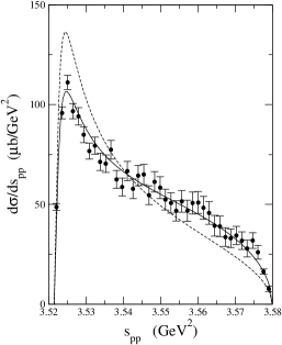
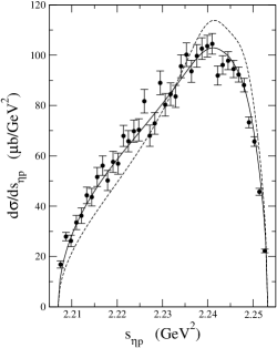
Figure 1: Invariant mass distributions at Q=15.5 MeV; left panel: (pp)-mass plot; right panel: ($\eta$p)-mass plot. The data are from [4] the calculated curves are from [6].

Since the agreement with experiment presented in [5] is of similar quality, polarization experiments are required to discriminate between these two models. The prediction of the s-wave model [6] is that all polarization observables are bound to vanish. Any non-zero value for the analyzing power reveals the presence of higher partial waves [5].

In the above considerations final-state $\eta$p interaction has been ignored and an interesting question arises how much its inclusion can change the resulting invariant mass spectra. The $\eta$p interaction is poorly known but there have been suggestions that the corresponding scattering length might be as large as about 1 fm. This is still one order of magnitude smaller than the pp scattering length but the discrepancies in the invariant mass distribution in Fig. 1 are not large either. The purpose of this work is to shed some light on the possible role of the $\eta$p final-state interaction but to be able to do that we need a formalism in which all pair-wise interactions would be regarded on equal footing.

The plan of our presentation is as follows. In the next Section we start with the well known two-body case recalling the arguments leading to the derivation of the FSI enhancement factor. In Section 3 we generalize these ideas to the three-body case by utilizing the hypersherical harmonics approach. Finally, in Section 4 we verify our model by confronting the obtained results with the experimental data.

2 Two-body final-state interaction

Since the proton-proton final-state interaction is believed to be the dominant ingredient in the description of the $pp\to pp\eta$ reaction close to threshold, it is logical to begin with the two-body FSI problem. The basic idea how to account for final state interaction was put forward 50 years ago by Fermi, Watson, Migdal [7] and others (for a review cf. [8]) and is based on the observation that in many processes the interaction responsible for carrying the system from the initial to the final state is of such a short range that in the first approximation may be regarded as point like. As a prototype one may consider a meson (x) production reaction $NN\to NNx$. To generate the meson mass m in nucleon-nucleon collision a large momentum transfer is required between the initial and the final nucleons, which is typically of the order $\sqrt{Mm}$, with $M$ being the nucleon mass. The corresponding ”range” of the production interaction is therefore much shorter than the range of the interaction between the two final state nucleons. Although it is perfectly true that the final state NN interaction significantly distorts the NN wave function but in the transition matrix element the contribution from all but the smallest NN separations will be strongly suppressed and the main effect may be attributed to the change of the normalization of the wave function at zero separation. If the non-interacting NN pair is described by a plane wave $\textstyle{\rm e}^{-\imath\,\bm{k}\cdot\bm{r}}$, where $\bm{k}$ is the relative NN momentum ($\hbar=c=1$ units are used hereafter), to account for final state interaction the latter must be replaced in the transition matrix element by the complete NN wave function $\Psi^{-}(\bm{k},\bm{r})^{\dagger}$ satisfying outgoing spherical wave boundary condition at infinity. Nevertheless, for a point-like interaction, we may set

$$\Psi^{-}(\bm{k},\bm{r})^{\dagger}\approx\textstyle{\rm e}^{-\imath\,\bm{k}\cdot\bm{r}}\;C(k)$$ (1)

in the matrix element so that the final state interaction will be accounted for by multiplying the transition matrix element by the enhancement factor, defined as

$$C(k)\equiv\displaystyle\lim_{r\to 0}\;\Psi^{+}(-\bm{k},\bm{r})/\textstyle{\rm e}^{-\imath\,\bm{k}\cdot\bm{r}}.$$ (2)

The factor $|C(k)|^{2}$ that appears in the cross section represents the ratio of two probabilities: one of finding the interacting NN pair at zero separation, while the other probability is associated with non-interacting particles. By construction, when the final state interaction is turned off, the enhancement factor will be equal to unity. Expanding both, the numerator and the denominator on the right hand side of (2) in partial waves, we have

$$C(k)=\displaystyle\lim_{r\to 0}\dfrac{\sum_{\ell=0}^{\infty}\;(2\ell+1)\,\imath^{-\ell}\,\psi_{\ell}(k,r)/r\;P_{\ell}(\hat{\bm{k}}\cdot\hat{\bm{r}})}{\sum_{\ell=0}^{\infty}\;(2\ell+1)\,\imath^{-\ell}\;j_{\ell}(kr)\,P_{\ell}(\hat{\bm{k}}\cdot\hat{\bm{r}})},$$ (3)

where $\psi_{\ell}(k,r)\sim r^{\ell+1}$ for small $r$, $j_{\ell}(kr)$ is spherical Bessel function and $P_{\ell}(\hat{\bm{k}}\cdot\hat{\bm{r}})$ denotes Legendre polynomial. Clearly, in the limit $r\to 0$ in (3), all higher partial waves will be suppressed by the centrifugal barrier, and only the contribution the from s-wave survives. Thus, we obtain a simple formula

$$C(k)=\psi_{0}(k,0)^{\prime}/k,$$ (4)

where prime denotes derivative with respect to $r$, and, as apparent from (4), the enhancement factor is determined by the slope of the wave function at the origin. To find this slope we must know the NN s-wave interaction and for simplicity we shall in the following assume that the latter takes the form of a spherically symmetric radial potential. The shape of this potential may be arbitrary but it must be of a short range. Given the NN potential, we can integrate outward the appropriate wave equation, containing both the nuclear and the Coulomb potential, generating numerically a regular solution $u_{0}(k,r)$ (i.e. vanishing at the origin) whose derivative for later convenience is selected to be

$$u_{0}(k,0)^{\prime}=C_{0}(\eta)\,k,$$ (5)

where $\eta$ denotes the Sommerfeld parameter and $C_{0}(\eta)^{2}=2\pi\eta/[\exp(2\pi\eta)-1]$ is the Coulomb barrier penetration factor. The sought for physical solution $\psi_{0}(k,r)$ occurring in (4) which is also regular, is necessarily proportional to $u_{0}(k,r)$, and, more explicitly, we have

$$\psi_{0}(k,r)=[C(k)/C_{0}(\eta)]\;u_{0}(k,r).$$ (6)

Now, all we need to calculate $C(k)$ is the asymptotic expression for the physical wave function. For $r=R$ with R much bigger than the range of the nuclear potential, the physical wave function takes the form

$$\psi_{0}(k,R)=F_{0}(\eta,kR)+f_{0}(k)\,H^{+}_{0}(\eta,kR),$$ (7)

where $H^{+}_{0}(\eta,kR)=G_{0}(\eta,kR)+\imath\,F_{0}(\eta,kR)$ with $G_{0}(\eta,kR)$ and $F_{0}(\eta,kR)$ being the standard Coulomb wave functions defined in [9], and $f_{0}(k)=\sin\delta\,\textstyle{\rm e}^{\imath\delta}$ denotes the s-wave scattering amplitude with $\delta$ being the s-wave Coulomb distorted phase shift. The differentiation of (7) with respect to R, provides us with a second condition for the derivatives but it should be noted that $u_{0}(k,R)$ and $u(k,R)^{\prime}$ occurring in these two matching conditions are to be regarded as known quantities. Indeed, they are fully specified by the boundary condition at the origin (5) and can be either calculated analytically, or obtained by numerical methods. Therefore, we end up with two algebraic equations in which the two unknowns are the enhancement factor $C(k)$ and the scattering amplitude $f_{0}(k)$ and the respective solutions, can be conveniently written as

$$C(k)=\dfrac{k\,C_{0}(\eta)}{w[H^{+}_{0}(\eta,kR),u_{0}(k,R)]},$$ (8)

and

$$f_{0}(k)=-\dfrac{w[F_{0}(\eta,kR),u_{0}(k,R)]}{w[H^{+}_{0}(\eta,kR),u_{0}(k,R)]},$$ (9)

where the symbol $w[f,g]$ denotes the Wronskian defined as $w[f,g]\equiv fg^{\prime}-f^{\prime}g$. The specific Wronskian occurring in the denominators of (8)–(9) has been referred to as the Jost function [8]. Thus, given the potential, the two-body enhancement factor can be obtained from (8).

3 Three-body final-state interaction

We wish now to extend the ideas outlined above to the three-body case. We assume that the pair-wise short range interaction between the particles is strong but the system is Borromean, i.e. no binary bound state may exist in the three-body system under consideration. A formal theory of the continuum in a Borromean system was developed in [10] using the same hyperspherical harmonics method which has been widely employed for the investigation of bound states and specifically the halo nuclei [11]. In this paper we follow this approach to derive the enhancement factor for three interacting particles. The wave functions in the continuum are solutions to the three-body problem satisfying the correct boundary conditions at infinity where the three-body asymptotics is most naturally expressed in terms of the rotationally and permutationally invariant hyperradius $\rho$ defined as the square root of the sum of squares of the inter-particle distances. Since the hyperradius reflects the size of the three-body system, similarly as in the two-body case, the enhancement factor may be obtained as the limiting value $\rho\to 0$ of the three-body wave function. The method of hyperspherical harmonics has been well documented in the literature, but to make this paper self-contained we wish to summarize briefly the theoretical framework necessary to treat the continuum of a Borromean system.

3.1 Coordinate sets and hyperspherical harmonics

For assigned particle positions $(\mathbf{r}_{1},\mathbf{r}_{2},\mathbf{r}_{3})$ and masses $(m_{1},m_{2},m_{3})$, the translationally invariant normalized sets of Jacobi coordinates $\mathbf{x}_{i},\mathbf{y}_{i}$ are defined, as follows

$$\mathbf{x}_{i} = \sqrt{\dfrac{m_{j}\,m_{k}}{(m_{j}+m_{k})\,\mu}}\,(\mathbf{r}_{j}-\mathbf{r}_{k}),$$ (10a)

$$\mathbf{y}_{i} = \sqrt{\dfrac{m_{i}\,(m_{j}+m_{k})}{\mu\,M}}\,\left(\mathbf{r}_{i}-\dfrac{m_{j}\,\mathbf{r}_{j}+m_{k}\,\mathbf{r}_{k}}{m_{j}+m_{k}}\right),$$ (10b)

$$\mathbf{R} = (m_{i}\mathbf{r}_{i}+m_{j}\mathbf{r}_{j}+m_{k}\mathbf{r}_{k})/M,$$ (10c)

where $\{i,j,k\}$ is a permutation of the particle labels $\{1,2,3\}$, $M=m_{1}+m_{2}+m_{3}$, and $\mu$ denotes an arbitrary mass which just sets the mass scale. Each of the three equivalent pairs $(\mathbf{x}_{i},\mathbf{y}_{i})$ together with the center of mass coordinate $\mathbf{R}$ describes the system. The transformation between different sets of Jacobi coordinates is referred to as a kinematical rotation and takes the form

$$\binom{\mathbf{x}_{j}}{\mathbf{y}_{j}}=\begin{pmatrix}\text{-}\cos\omega_{ij}&\text{ }\sin\omega_{ij}\\ \text{-}\sin\omega_{ij}&\text{-}\cos\omega_{ij}\end{pmatrix}\binom{\mathbf{x}_{i}}{\mathbf{y}_{i}}$$ (11)

where the rotation angle, confined by $-\pi/2\leq\omega_{ij}\leq\pi/2$, is given by

$$\omega_{ij}=\arctan\left[\sigma\{i,j,k\}\sqrt{M\,m_{k}/m_{i}\,m_{j}}\right],$$ (12)

with $\sigma\{i,j,k\}$ denoting the sign of the permutation $\{i,j,k\}$.

The Jacobi momenta $\mathbf{k}_{i},\mathbf{q}_{i}$ and $\mathbf{P}$, canonically conjugate to $\mathbf{x}_{i},\mathbf{y}_{i}$ and $\mathbf{R}$, respectively, are defined by the relations,

$$\mathbf{k}_{i} = \sqrt{\dfrac{m_{j}\,m_{k}\,\mu}{m_{j}+m_{k}}}\,\left(\frac{\mathbf{p}_{j}}{m_{j}}-\frac{\mathbf{p}_{k}}{m_{k}}\right),$$ (13a)

$$\mathbf{q}_{i} = \sqrt{\dfrac{(m_{j}+m_{k})m_{i}\mu}{M}}\,\left(\frac{\mathbf{p}_{i}}{m_{i}}-\frac{\mathbf{p}_{j}+\mathbf{p}_{k}}{m_{j}+m_{k}}\right),$$ (13b)

$$\mathbf{P} = \mathbf{p}_{1}+\mathbf{p}_{2}+\mathbf{p}_{3},$$ (13c)

where $\mathbf{p}_{i}\;(i=1,2,3)$ are the laboratory frame momenta.

Instead of the Jacobi coordinates we shall use hyperspherical coordinates comprising of a hyperradius $\rho$ and five angles. The hyperradius $\rho$ determines the size of a three–body system and is invariant with respect to kinematic rotations

$$\rho^{2}=x_{i}^{2}+y_{i}^{2},\qquad i=1,2,3.$$ (14)

The five angular variables forming a five-dimensional solid angle $\Omega_{\rho}$ include the usual angles $(\theta_{x}^{i},\phi_{x}^{i})$, $(\theta_{y}^{i},\phi_{y}^{i})$ specifying the unit vectors $\hat{{\bf x}}_{i}$, $\hat{{\bf y}}_{i}$ and these are supplemented by the hyperangle $\alpha_{i}$ defined by the equalities

$$x_{i}=\rho\sin\alpha_{i},\qquad y_{i}=\rho\cos\alpha_{i},$$ (15)

where $0\leq\alpha_{i}\leq\pi/2$. The five-dimensional volume element d$\Omega_{\rho}$ is

$$\textstyle{\rm d}\Omega_{\rho}=\sin^{2}\alpha_{i}\,\cos^{2}\alpha_{i}\,\textstyle{\rm d}\alpha_{i}\,\textstyle{\rm d}\hat{\bf x}_{i}\,\textstyle{\rm d}\hat{\bf y}_{i}.$$ (16)

For the conjugate momenta, we proceed in a similar fashion introducing the hypermomentum $\kappa$ and the associated hyperangle $\beta_{i}$

$$k_{i}=\kappa\sin\beta_{i},\qquad q_{i}=\kappa\cos\beta_{i},$$ (17)

where owing to the energy conservation $Q=\kappa^{2}/2\mu$.

In the six-dimensional space, the kinetic energy operator $\hat{T}$ takes a separable form

$$\hat{T}=-\frac{1}{2\mu}\left(\dfrac{\partial^{2}}{\partial\rho^{2}}+\dfrac{5}{\rho}\dfrac{\partial}{\partial\rho}-\dfrac{1}{\rho^{2}}\hat{K}^{2}\right),$$ (18)

where the hypermomentum operator $\hat{K}$ is the generator of rotations in the six-dimensional space. The operator $\hat{K}^{2}$ takes the form

$$\hat{K}^{2}=-\dfrac{\partial^{2}}{\partial\alpha_{i}^{2}}-4\cot(2\alpha_{i})\dfrac{\partial}{\partial\alpha_{i}}+\dfrac{\hat{\bm{l}}_{i}^{2}}{\sin^{2}\alpha_{i}}+\dfrac{\hat{\bm{\lambda}}_{i}^{2}}{\cos^{2}\alpha_{i}},$$ (19)

where the angular momentum operators $\hat{\bm{l}}_{i}$ and $\hat{\bm{\lambda}}_{i}$ occurring in (19), are defined as

$$\hat{\bm{l}}_{i}=-\imath\,\bm{x}_{i}\times\,\dfrac{\partial}{\partial\,\bm{x}_{i}},\qquad\hat{\bm{\lambda}}_{i}=-\imath\,\bm{y}_{i}\times\,\dfrac{\partial}{\partial\,\bm{y}_{i}},$$ (20)

and $\hat{\bm{l}}_{i}^{2}$ and $\hat{\bm{\lambda}}_{i}^{2}$ have eigenvalues $\ell(\ell+1)$ and $\lambda(\lambda+1)$, respectively. The operator (19) has eigenvalues $K(K+4)$ where $K=2n+\ell+\lambda$ for integer $n$. The quantum number $K$ has been dubbed hypermomentum, its value is the same in all three Jacobi systems, and the corresponding eigenfunctions are known as hyperspherical harmonics (abbreviated HH hereafter).

From now on we choose set 3 as the basic one and to simplify notation in the following we will suppress the label referring to our particular choice of the Jacobi system. The HH have the explicit form

$${\cal Y}_{KLM_{L}}^{\ell\lambda}\left(\Omega_{\rho}\right)=\chi_{K}^{\ell\lambda}(\alpha)\left[Y_{\ell}(\hat{\bf x})\otimes Y_{\lambda}(\hat{\bf y})\right]_{LM_{L}},$$ (21)

where $L$ is the total angular momentum resulting from vector addition $\bm{L}=\bm{l}+\bm{\lambda}$. In (21) the symbol $\Omega_{\rho}$ denotes collectively all five angular variables with $Y_{lm}$ being the usual spherical harmonics. The square bracket in (21) indicates vector coupling of $\mathbf{l}$ and $\bm{\lambda}$ producing a total angular momentum $\mathbf{L}$ and the appropriate quantum numbers associated with the latter operator are $L$ and $M_{L}$. In (21), the hyperangular eigenfunctions are

$$\chi_{K}^{\ell\lambda}(\alpha)=N_{K}^{\ell\lambda}\;\sin^{\ell}\alpha\,\cos^{\lambda}\alpha\,P_{n}^{\ell+\!\!\textstyle{\frac{1}{2}},\scriptstyle\lambda+\!\!\textstyle{\frac{1}{2}}}(\cos 2\alpha),$$

where $P_{n}^{\alpha,\beta}(x)$ are the Jacobi polynomials (cf. [9]) and $N_{K}^{\ell\lambda}$ is the normalization constant. The HH in (21) are orthonormalized using the volume element (16) and $\alpha$ stands for any of the $\alpha_{i}$.

For clarity reasons, to avoid unnecessary complications, we are going to restrict our considerations to the simplest case when the particles have no internal degrees of freedom. When the particles are moving freely the spacial part of the three-particle wave-function will be described in the c.m. frame by a plane wave, whose HH expansion can be written as

$$\textstyle{\rm e}^{\imath\mathbf{k}\cdot\mathbf{x}+\imath\mathbf{q}\cdot\mathbf{y}}=\dfrac{(2\pi)^{3}}{(\kappa\rho)^{5/2}}\,\displaystyle\sum_{LM_{L}K\ell\lambda}\;{\cal Y}^{\ell\lambda}_{KLM_{L}}(\Omega_{\rho})\;\imath^{K}\,\sqrt{\kappa\rho}\,J_{K+2}(\kappa\rho)\;{\cal Y}^{\ell\lambda}_{KLM_{L}}(\Omega_{\kappa})^{\dagger},$$ (22)

where $J_{K+2}$ denotes Bessel function of integer order and solid angle $\Omega_{\kappa}$ comprises five angular variables that specify the directions of the incident momenta in the six-dimensional space. It is worth noting that since the radial part in (22) depends solely upon $K$, the plane wave is an invariant under six-dimensional rotations. The two-body interactions break up this invariance and for interacting particles the three-particle wave function in the continuum $\Psi_{\mathbf{k},\mathbf{q}}(\mathbf{x},\mathbf{y})$ will have a more complicated HH expansion. For the simplest case of pair-wise central potentials depending upon the particle separations, we have

$$\Psi_{\mathbf{k},\mathbf{q}}(\mathbf{x},\mathbf{y})=\dfrac{(2\pi)^{3}}{(\kappa\rho)^{5/2}}\sum{\cal Y}^{\ell\lambda}_{KLM_{L}}(\Omega_{\rho})\;\psi^{L}_{K\ell\lambda,\tilde{K}\tilde{\ell}\tilde{\lambda}}(\kappa,\rho)\;{\cal Y}^{\tilde{\ell}\tilde{\lambda}}_{\tilde{K}LM_{L}}(\Omega_{\kappa})^{\dagger}$$ (23)

where the summation indices are $L,M_{L},K,\ell,\lambda,\tilde{K},\tilde{\ell},\tilde{\lambda}$ and the normalization condition reads

$$\int\Psi_{\mathbf{k^{\prime}},\mathbf{q^{\prime}}}(\mathbf{x},\mathbf{y})^{\dagger}\;\Psi_{\mathbf{k},\mathbf{q}}(\mathbf{x},\mathbf{y})\;\textstyle{\rm d}^{3}x\,\textstyle{\rm d}^{3}y=\delta(\mathbf{k}^{\prime}-\mathbf{k})\,\delta(\mathbf{q}^{\prime}-\mathbf{q}).$$ (24)

In the expansion (23), only the total three-particle angular momentum L is a good quantum number and the as yet unspecified hyperradial part $\psi^{L}_{K\ell\lambda,\tilde{K}\tilde{\ell}\tilde{\lambda}}(\kappa,\rho)$ must be determined from the underlying three-body dynamics. The dependence upon the tilded indices, associated with the incident momenta, enters solely via the asymptotic boundary condition at $\rho\to\infty$. The full wave-function $\Psi_{\mathbf{k},\mathbf{q}}(\mathbf{x},\mathbf{y})$ is a solution to the three-body Schrödinger equation

$$(\hat{T}+\hat{V}-Q)\Psi_{\mathbf{k},\mathbf{q}}(\mathbf{x},\mathbf{y})=0,$$ (25)

with $\hat{V}=\hat{V}_{12}+\hat{V}_{23}+\hat{V}_{31}$ where $\hat{V}_{ij}$ stands for the pair-wise interaction between particles $i$ and $j$. Inserting (23) in (25) and projecting onto the hyperangular part of the wave function, results in an infinite set of coupled systems of differential equations enumerated by the conserved total angular momentum $L$ – the only quantum number that does not mix. For an assigned $L$, we have

$$\begin{split}\left\{\dfrac{\textstyle{\rm d}^{2}}{\textstyle{\rm d}\rho^{2}}-\dfrac{(K+3/2)(K+5/2)}{\rho^{2}}+\kappa^{2}\right\}\;\psi^{L}_{K\ell\lambda,\tilde{K}\tilde{\ell}\tilde{\lambda}}(\kappa,\rho)=\hskip 91.04742pt\\ =2\mu\sum_{K^{\prime}\ell^{\prime}\lambda^{\prime}}\langle K^{\prime}\ell^{\prime}\lambda^{\prime}|\hat{V}|K\ell\lambda\rangle\;\;\psi^{L}_{K^{\prime}\ell^{\prime}\lambda^{\prime},\tilde{K}\tilde{\ell}\tilde{\lambda}}(\kappa,\rho),\end{split}$$ (26)

and we are left with a multi-channel situation where each channel is specified by three quantum numbers $\{K\ell\lambda\}$. Each system of equations (26) with $L=0,1,2,\dots$ is infinite because there is no upper limit for $K$, and, therefore, for practical reasons $K$ must be truncated at some finite value $K_{max}$ so that the orbital momenta $\ell$ and $\lambda$ are thereby restricted to vary in finite limits. The value of $K_{max}$ determines the order of the approximation and must be be large enough to ensure the convergence of the method. It should be noted that in (26) the potential term has been sandwiched between the HH functions ${\cal Y}^{\ell\lambda}_{KLM_{L}}(\Omega_{\rho})$ and after integration over the five angular variables $\Omega_{\rho}$, these matrix elements depend solely upon the hyperadius $\rho$

$$\langle K^{\prime}\ell^{\prime}\lambda^{\prime}|\hat{V}|K\ell\lambda\rangle=\int{\cal Y}^{\ell^{\prime}\lambda^{\prime}}_{K^{\prime}LM_{L}}(\Omega_{\rho})^{\dagger}\;\sum_{j=1}^{3}\sum_{i\neq j}^{3}V_{ij}(\rho,\Omega_{\rho})\;{\cal Y}^{\ell\lambda}_{KLM_{L}}(\Omega_{\rho})\;\textstyle{\rm d}\,\Omega_{\rho}.$$ (27)

With the adopted here set 3 of HH, the computation of the potential matrix element $\hat{V}_{12}$ is relatively straightforward because the separation vector between particles 1 and 2 is proportional to $|\mathbf{x}|$ and the calculation of the potential matrix involves a single integration. By contrast, in the two remaining potentials the corresponding separations, $r_{23}$ and $r_{31}$, respectively, are linear combinations of the two vectors $\mathbf{x}$ and $\mathbf{y}$ which unavoidably leads to five-dimensional integrations in the calculation of the potential matrix. Fortunately, there is a very efficient procedure to overcome this difficulty, based on the observation that all HH with fixed $(K,L)$ values defined with respect to set $i$ (cf. (10)) are linear combinations of HH belonging a set $j$ and this transformation is effected by means of the so called Raynal-Revai (RR) coefficients [12], viz.

$${\cal Y}^{\ell_{i}\lambda_{i}}_{KLM_{L}}(\alpha_{i},\mathbf{\hat{x}}_{i},\mathbf{\hat{y}}_{i})=\sum_{\ell_{j}\,\lambda_{j}}\langle\ell_{j}\,\lambda_{j}|\ell_{i}\,\lambda_{i}\rangle_{KL}\;{\cal Y}^{\ell_{j}\lambda_{j}}_{KLM_{L}}(\alpha_{j},\mathbf{\hat{x}}_{j},\mathbf{\hat{y}}_{j}),$$ (28)

where the RR coefficients $\langle\ell_{j}\,\lambda_{j}|\ell_{i}\,\lambda_{i}\rangle_{KL}$ are functions of the angle specifying the kinematic rotation $i\to j$ given in (12). With the aid of (28), the potential matrix of $\hat{V}_{23}$ may be computed in basis $1$ where this task is simple and subsequently transformed to basis $3$.

The radial wave functions must be regular at $\rho=0$ and the boundary condition imposed on the solutions of (26) is

$$\psi_{K\ell\lambda,\tilde{K}\tilde{\ell}\tilde{\lambda}}^{L}(\kappa,\rho)\sim\rho^{K+5/2}\qquad\text{for}\qquad\rho\to 0.$$ (29)

For $\rho\to\infty$ the potential term in (26) goes to zero so that in this limit the system of equations (26) becomes decoupled. In absence of the potential term, the asymptotic solutions of the radial equations are well known, they are given in terms of the Bessel and Neuman functions [9] $J_{K+2}(\kappa\rho)$ and $Y_{K+2}(\kappa\rho)$, respectively. With the Coulomb interaction present, for large $\rho$ strong interaction potentials become negligible, and we set

$$\lim_{\rho\to\infty}\psi_{K\ell\lambda,\tilde{K}\tilde{\ell}\tilde{\lambda}}^{L}(\kappa,\rho)=\delta_{K\tilde{K}}\,\delta_{\lambda\tilde{\lambda}}\,\delta_{\ell\tilde{\ell}}\;F_{\cal L}(\eta,\kappa\rho)+\langle K\ell\lambda|{\cal T}^{L}|\tilde{K}\tilde{\ell}\tilde{\lambda}\rangle\;H^{+}_{\cal L}(\eta,\kappa\rho),$$ (30)

with

$$H^{+}_{\cal L}(\eta,\kappa\rho)=G_{\cal L}(\eta,\kappa\rho)+\imath\,F_{\cal L}(\eta,\kappa\rho).$$ (31)

where we have extended the standard definition of Coulomb wave functions so that the orbital quantum number $\ell$ which takes on integer values is replaced by ${\cal L}=K+3/2$ with half-integer ${\cal L}$. The T-matrix occurring in (30) $\langle K\ell\lambda|{\cal T}^{L}|\tilde{K}\tilde{\ell}\tilde{\lambda}\rangle$ describes $3\to 3$ scattering processes and is similar to that encountered in the two-body multichannel problem. In particular, it can be diagonalized which allows to determine the appropriate eigenphases $\delta_{LK\ell\lambda}$ whose rapid variation with energy indicates a resonance.

3.2 Three-body final-state interaction enhancement factor

The formalism developed in the preceding subsection will be now applied to calculate the enhancement factor describing final-state interaction between three particles in a Borromean system. The approximation scheme will be based on the assumption that all interactions are of a short range and therefore the most important effect comes from the distortion of the wave function at very small separations. Bigger separation region is strongly suppressed by the small size of the interaction volume and gives relatively small contribution to the overlap integrals representing reaction transition amplitudes. Thus, similarly as in the two-body case, we shall define the enhancement factor as the limit reached by the square of the absolute value of the ratio – the full three-body wave function divided by the plane wave – when the size of the system represented by $\rho$ goes to zero. It is apparent from (26) that the role of the centrifugal barrier plays now the quantum number $K$ and the leading term in the wave function in the limit $\rho\to 0$ has $K=0$ implying that $\ell=\lambda=0$ and $L=0$. Therefore, we confine our attention solely to the $L=0$ set (26) where significant simplifications take place, namely we have $\lambda=\ell$ and $K$ necessarily even: $K=2(n+\ell)$.

Formally, the three-particle enhancement factor will be defined as the limit

$$F(\bm{k},\bm{q})=\lim_{\rho\to 0}\left|\dfrac{\Psi_{\mathbf{k},\mathbf{q}}(\mathbf{x},\mathbf{y})}{\textstyle{\rm e}^{\imath\mathbf{k}\cdot\mathbf{x}+\imath\mathbf{q}\cdot\mathbf{y}}}\right|^{2},$$ (32)

which by making use of (22) and (23), simplifies to the form

$$F(\bm{k},\bm{q})=\lim_{\rho\to 0}\left|\sum_{\tilde{K},\tilde{\ell}}\;\dfrac{\psi^{0}_{000,\tilde{K}\tilde{\ell}\tilde{\ell}}(\kappa,\rho)}{\sqrt{\kappa\rho}\,J_{2}(\kappa\rho)}\;\;{\cal Y}^{\tilde{\ell}\tilde{\ell}}_{\tilde{K}00}(\Omega_{\kappa})^{\dagger}\right|^{2},$$ (33)

where we have dropped the uninteresting constant factor $|{\cal Y}^{00}_{000}(\Omega_{\rho})|^{2}$. To obtain the enhancement factor it is sufficient to calculate the radial wave function $\psi^{0}_{000,\tilde{K}\tilde{\ell}\tilde{\ell}}(\kappa,\rho)$ for small $\rho$ and take the limit indicated in (33).

The calculation of the radial wave function is carried out similarly as for the two-body case except that scalar quantities now need to be replaced by matrices in channel space. These channels are specified by two quantum numbers ${K\ell}$ but to simplify the notation it is possible to use a single integer $\nu=\textstyle{\frac{1}{2}}\;(\textstyle{\frac{1}{2}}K)(\textstyle{\frac{1}{2}}K+1)+\ell+1$ enumerating all the states under consideration ($\nu$=1,2,3…). Truncating the infinite sequence of $K$ values at some assigned $K_{max}$, the total number of channels $N$ is

$$N=\textstyle{\frac{1}{2}}(\textstyle{\frac{1}{2}}K_{max}+1)(\textstyle{\frac{1}{2}}K_{max}+2),$$ (34)

and we have to solve $N$ second order differential equations given in (26). The physical solution of (26) can be envisaged as a column vector in channel space. To obtain the physical solution we must first generate numerically $N$ linearly independent particular solutions vanishing at the origin with an arbitrary slope at $\rho=0$. These $N$ solutions can be grouped together to form the $N$ columns of a single $N\times N$ square matrix $\bm{\Phi}$ (hereafter we denote matrices by boldface symbols). In practice, this matrix may be obtained by solving $N$ times the system of equations (26) imposing for small $\rho$ the boundary condition

$$\Phi_{K\ell,\tilde{K}\tilde{\ell}}(\kappa,\rho)=\delta_{K\tilde{K}}\,\delta_{\ell\tilde{\ell}}\,(\kappa\rho)^{K+5/2},$$ (35)

so that these particular solutions will be enumerated by two quantum numbers $\tilde{K}\tilde{\ell}$. Since the columns of $\bm{\Phi}$ are linearly independent, they span the space of all possible slopes. Therefore, any column vector solution $\psi$ of (26) must be expressible as some linear combination of the N columns of $\bm{\Phi}$, and we have

$$\psi(\rho)=\bm{\Phi}(\rho)\cdot c,$$ (36)

with $c$ denoting a column vector of constant coefficients.

The matrix of physical solutions occurring in (33) differs from $\bm{\Phi}$ at most by a constant matrix and the latter will be explicitly determined by making use of the boundary condition for asymptotic $\rho$. For large $\rho$ the physical solution must be of the form

$$\bm{\Psi}(\kappa,\rho)=\bm{F}(\kappa\rho)+\bm{H}^{+}(\kappa\rho)\cdot\bm{T}(\kappa),$$ (37)

where $\bm{T}$ is the true $3\to 3$ scattering matrix. In formula (37) $\bm{F}$ denotes a diagonal matrix containing the regular solutions $F_{\cal L}(\eta,\kappa\rho)$ of (26) in absence of the strong interaction, whereas $\bm{H}^{+}$ is another diagonal matrix containing outgoing hyperspherical waves $G_{\cal L}(\eta,\kappa\rho)+\imath\,F_{\cal L}(\eta,\kappa\rho)$. Since $\bm{\Phi}$ is proportional to $\bm{\Psi}$, for some large $\rho=\rho_{m}$, we may set the following matching condition for the wave functions and their derivatives

$$\bm{\Phi}(\kappa,\rho_{m})\cdot\bm{C}(\kappa) = \bm{F}(\kappa\rho_{m})+\bm{H}^{+}(\kappa\rho_{m})\cdot\bm{T}(\kappa),$$ (38a)

$$\bm{\Phi}(\kappa,\rho_{m})^{\prime}\cdot\bm{C}(\kappa) = \bm{F}(\kappa\rho_{m})^{\prime}+\bm{H}^{+}(\kappa\rho_{m})^{\prime}\cdot\bm{T}(\kappa),$$ (38b)

where prime denotes derivative with respect to $\rho$ and $\bm{C}(\kappa)$ is a constant (albeit energy dependent) matrix to be determined. Eliminating $\bm{T}$ between the two matrix equations (38), we obtain

$$\bm{C}(\kappa)=\dfrac{2\kappa}{\pi}[\bm{H}^{+}(\kappa\rho_{m})\cdot\bm{\Phi}(\kappa,\rho_{m})^{\prime}-\bm{H}^{+}(\kappa\rho_{m})^{\prime}\cdot\bm{\Phi}(\kappa,\rho_{m})]^{-1},$$ (39)

and $\bm{C}(\kappa)$ is seen to be proportional to the inverse of the Jost matrix. Clearly, formula (39) may be viewed as a three-body extension of (8). Because the matrix $\bm{C}(\kappa)$ involves the inverse of the Jost determinant it is bound to have the same singularity structure as the T-matrix.

The physical solution can be now expressed entirely in terms of $\bm{\Phi}$

$$\bm{\Psi}(\kappa,\rho)=\bm{\Phi}(\kappa,\rho)\cdot\bm{C}(\kappa)$$ (40)

and the limiting procedure $\rho\to 0$ in (33) may be effected with the aid of (35). Similarly as in the two-body case, the only terms in the summations giving non-vanishing contribution are those with $K=0$. Leaving out irrelevant numerical factor, the enhancement factor in (33) takes the form

$$F(\bm{k},\bm{q})=F(-\bm{k},-\bm{q})=\left|\sum_{K\ell}c_{K\ell}(\kappa)\;{\cal Y}^{\ell\ell}_{K00}(\Omega_{\kappa})\right|^{2},$$ (41)

where the expansion coefficients $c_{K\ell}(\kappa)$ are provided as the first row of the matrix $\bm{C}(\kappa)$ given in (39).

Formula (41) gives the enhancement factor in the form of an expansion in an orthonormal set of momentum dependent HH functions which turns out to be quite useful in effecting phase space integrations. We shall illustrate this point for the case when the transition matrix is assumed to be constant so that the cross section is essentially determined by the enhancement factor. The integration over the five angles $\textstyle{\rm d}\Omega_{\kappa}$, yields the total cross section

$$\sigma(\kappa)\sim\dfrac{\kappa^{4}}{f(\kappa)}\;\sum_{K\ell}|c_{K\ell}(\kappa)|^{2},$$ (42)

where $\kappa^{4}$ results from phase space and $f(\kappa)$ denotes the incident flux factor. The summation over $K$ extends over all even numbers from 0 up to $K_{max}$ and in the following we take it to be the value at which the convergence has been attained.

When the incident energy is fixed (i.e, $\kappa$ is a constant), the quantities of interest are usually the effective mass distributions, or equivalently, the corresponding kinetic energy distributions of the different pairs in their c.m frame. Such distributions are obtained here by integrating only over the directions of $\bm{k}$ and $\bm{q}$ retaining the dependence upon the two remaining variables, $\kappa$ and $\beta$. With our choice of 3 as the basic Jacobi set, the distribution of the center of mass energy $T_{3}$ of the pair $\{12\}$, takes particularly simple form

$$\dfrac{\textstyle{\rm d}\sigma}{\textstyle{\rm d}T_{3}}=\sqrt{T_{3}(Q-T_{3})}\,\sum_{K^{\prime}K\ell}c_{K^{\prime}\ell}(\kappa)^{*}\,c_{K\ell}(\kappa)\,\chi^{\ell\ell}_{K^{\prime}}(\beta)\,\chi^{\ell\ell}_{K}(\beta),$$ (43)

where $T_{3}=Q\,\sin^{2}\beta$ and the square root factor is a remanet of the phase space. All other factors that depend only upon $\kappa$ have been dropped as they may be absorbed in the arbitrary normalization constant. The calculation of c.m kinetic energy distributions of the two remaining pairs, i.e $\{23\}$ and $\{31\}$, respectively, may be carried out in exactly the same manner but the HH occurring in (41) need to be first transformed to the appropriate Jacobi system by applying a kinematical rotation. Thus, using the transformation (28) in (41), the distribution of the kinetic energy of the $\{23\}$ pair, $T_{1}$, is

$$\begin{split}\dfrac{\textstyle{\rm d}\sigma}{\textstyle{\rm d}T_{1}}=\sqrt{T_{1}(Q-T_{1})}\;\sum_{K^{\prime}K\ell^{\prime}_{3}\ell_{3}\ell_{1}}c_{K^{\prime}\ell^{\prime}_{3}}(\kappa)^{*}\,c_{K\ell_{3}}(\kappa)\,\chi^{\ell_{1}\ell_{1}}_{K^{\prime}}(\beta_{1})\,\chi^{\ell_{1}\ell_{1}}_{K}(\beta_{1})\times\\ \times\;\langle\ell_{1}\ell_{1}|\ell_{3}\ell_{3}\rangle_{K0}\;\langle\ell_{3}^{\prime}\ell_{3}^{\prime}|\ell_{1}\ell_{1}\rangle_{K^{\prime}0},\hskip 45.52718pt\end{split}$$ (44)

where $T_{1}=Q\,\sin^{2}\beta_{1}$ and the corresponding distribution of $T_{2}$ follows from (44) in result of $P_{12}$ permutation. It should be perhaps clarified that this permutation in general changes the kinematic rotation angle that enters the RR coefficients and in consequence the $T_{2}$ distribution does not have to be the same as that given in (44).

4 Comparison with experiment and conclusions

In the preceding section our considerations have been quite general and now we wish to apply this theory to the investigation of FSI effects in the $pp\to pp\eta$ reaction close to threshold. To simplify matters we assume that the excitation energy is sufficiently low so that the total orbital momentum in the final state is zero and the $\mbox{}^{3}P_{0}\to\mbox{}^{1}S_{0}\,s$ transition amplitude is the sole contributor to the cross section. We label the two protons as 1 and 2, respectively, and the meson as 3 choosing Jacobi set 3 for all computations. With the two protons in a singlet state, Pauli principle requires that in this frame the orbital momenta $\ell_{3},\lambda_{3}$ take only even values. This guarantees that the spatial part wave function will be symmetric with respect to the $\{12\}$ permutation. We have tried several possible forms of the pp potential in the ${}^{1}S_{0}$ state: a delta-shell, a Gaussian or a fully realistic Reid potential (for details cf. [6]). The $\eta$-p interaction is poorly known, for the real part of the scattering length values between 0.2 and about 1.0 fm have been suggested [13]. Additional difficulty stems from the multi-channel nature of this interaction: already at threshold there are open channels so that $\eta$p scattering length is a complex number. At present there is not enough information to include these additional channels into our formalism, therefore in this work $\eta$-p interaction has been simulated by the simplest non-absorptive delta-shell potential operative in the s-wave only whose range has been arbitrarily fixed to be 1 fm. The depth of this potential can be then adjusted as to yield an assigned value of the $\eta$p scattering length $a_{\eta p}$. Since the precise value of the latter is not available [13] we used three values 0.5, 1.0 and 1.5 fm, respectively, which we believe is a representative sample.

All our computations have been carried out for the lowest excitation energy equal Q=15.5 MeV for which two-particle invariant mass spectra are experimentally available. The system of equations (26) was perpetually solved by increasing successively in each step the value of $K_{max}$ until convergence has been attained. For delta-shell and Gaussian pp potentials this occurred at $K_{max}=24$ but with Reid potential this figure must be doubled. Similarly as in the two-body case [6] the results are completely insensitive to the shape of the pp potential. The results of our computations are presented in Fig. 2 where they are compared with the data from [4].

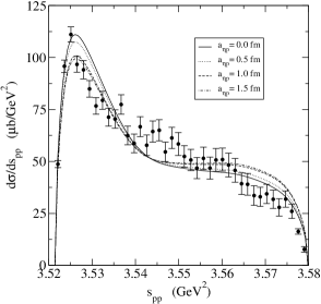
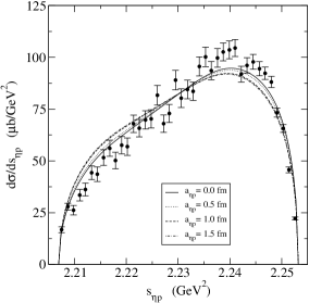
Figure 2: Invariant mass distributions at Q=15.5 MeV obtained from a three-body calculation: left panel pp pair; right panel $\eta$p pair. The data are from [4].

Not unexpectedly, the dominance of the pp interaction is apparent from both plots. Since the values of $a_{\eta p}>1\,fm$ are probably rather unrealistic [13], we may say that the $\eta$p interaction is of marginal importance as far as invariant mass distributions are concerned.

Comparing the invariant mass spectra obtained in the two-body approach (Fig. 1) with those resulting from the full three-body calculation (Fig. 2) we can see that even when the $\eta$p interaction is completely disregarded, the invariant mass plots are different in these two cases. Although the input in both approaches is the same but the underlying calculational schemes are different. Owing to the proper boundary condition (37) also in absence of $\eta$-p interaction the three-body wave function has entangled form, i.e it cannot be expressed as a product of the p-p wave function times a plane wave associated with the free propagation of the $\eta$. Since in the approximation using the two-body enhancement factor the very existence of the $\eta$ is unaccounted for, the latter does not depend upon the meson kinematics (in [6] we made an attempt to lift this deficiency by introducing ad hoc a linear dependence upon q). By contrast, even in absence of $\eta$-p interaction the three-body enhancement factor accounts for the $\eta$ propagation. In particular, the mass of the $\eta$ strongly influences the dynamics of the three-body system as can be seen from (10a) and (27).

The three-body calculation is in both spectra closer to experiment. We wish to note here that the curves presented in Fig. 2 and as well as the dashed curves from Fig. 1 contain no adjustable parameters except for the overall normalization. Our three-body calculation clearly favors smaller $a_{\eta p}$ values $a_{\eta p}\sim\,$ 0÷$0.5\,fm$. For $a_{\eta p}>0.5\,fm$ the height of the close to threshold peak in $s_{pp}$ plot in Fig. 2 is depressed which is accompanied by a build up of a pronounced shoulder at the high-energy end. At the same time another shoulder appears at the low-energy end in $s_{\eta p}$ distribution in Fig. 2. All these features worsen the agreement with experiment. Unfortunately, it would be difficult to improve the existing estimates of the $a_{\eta p}$ scattering length using the data displayed in Fig. 2, especially that absorptive effects have been ignored.

Summarizing, we have developed a general three-body formalism for calculating FSI effects in a three-particle final state. To the best of our knowledge, this is the first attempt in the literature to derive a three-body final-state interaction enhancement factor. The presented calculational framework employs the hypersherical harmonics method and is applicable for three-body systems in which no binary bound state can exist. The necessary input which must be provided are all three pairwise potentials. Detailed computations carried out for the $pp\to pp\eta$ reaction at Q=15.5 MeV show that in the invariant mass spectra the role of the $\eta$-p interaction is marginal and more important is the proper boundary condition imposed on the final-state wave function. The three-body calculations involving no adjustable parameters reproduce quite well the experimental invariant mass spectra.

Partial support under grant KBN 5B 03B04521 is gratefully acknowledged.

References

- [1] P. Moskal et al., Prog. Part. Nucl. Phys. 49 (2002) 1.
- [2] C. Hanhart, e-Print Archive: hep-ph/0311341.
- [3] M. Abdel-Bary et al., Eur. Phys. J. A 16 (2003) 127.
- [4] P. Moskal et al., Phys. Rev. C 69 (2004) 025203.
- [5] K. Nakayama et al., Phys. Rev. C68 (2003) 045201.
- [6] A. Deloff, Phys. Rev. C 69 (2004) 035206.
-
[7]
E. Fermi, Nuovo Cim., Suppl. Vol. II, No. 1 (1955) 17
K.M. Watson, Phys. Rev. 88 (1952) 1163; ibid. 89 (1953) 575;
A.B. Migdal, Zh. Exper. Theor. Fiz. 1 (1955) 17. -
[8]
M.L. Goldberger and K.M. Watson, Collision Theory, Wiley, N.Y.,
1964;
M. Froissart and R. Omnes, in Physique des Hautes Energies,
C. DeWitt and M. Jacob (eds.), Gordon & Breach, New York 1965;
J. Gillespie, Final state interactions, Holden-Dey, San Francisco 1964. - [9] M. Abramowitz and I.A. Stegun (eds.) Handbook of Mathematical Functions, Dover, New York, 1965.
- [10] B.V. Danilin and M.V. Zhukov, Phys. At. Nucl. 56 (1993) 460.
- [11] E. Nielsen, D.V. Fedorov, A.S. Jensen and E. Garrido, Phys. Rep. 347 (2001) 373.
- [12] J. Raynal and J. Revai, Nuovo Cim. A 68 (1970) 612.
- [13] A.M. Green and S. Wycech, Phys. Rev. C 55 (1997) 2167; ibid. C 60 (1999) 035208.