Gamow-Teller $GT_{+}$ distributions in nuclei with mass $A=90-97$

Abstract

We investigate the Gamow-Teller strength distributions in the electron-capture direction in nuclei having mass $A=90-97$, assuming a ⁸⁸Sr core and using a realistic interaction that reasonably reproduces nuclear excitation spectra for a wide range of nuclei in the region as well as experimental data on Gamow-Teller strength distributions. We discuss the systematics of the distributions and their centroids. We also predict the strength distributions for several nuclei involving stable isotopes that should be experimentally accessible for one-particle exchange reactions in the near future.

I Introduction

New frontiers of nuclear structure experiments to probe the Gamow-Teller distributions in medium-mass nuclei are currently being pursued. These experiments will be able to measure Gamow-Teller data in the mass 90-100 region. Extensive theoretical studies have been devoted to Gamow-Teller total strengths and strength distributions in $1s$-$0d$ shell nuclei (mass $A=16$-40 nuclei) BW-88 and the $0f$-$1p$ shell (mass $A=40$-80 nuclei) Langanke95 ; Martinez96 ; Caurier99GT . Due to an excellent agreement between shell model results and the available experimental data, the calculated results have been used extensively to predict numerous Gamow-Teller strength distributions in nuclei that have not yet become experimentally accessible Langanke00 .

In addition to their nuclear structure interests, an appropriate description of Gamow-Teller transitions in nuclei directly affects the early phases of type II supernova core collapse since electron capture rates are partly determined by them. The effects of the improved rate estimates are rather dramatic, as was recently discussed in Refs. Langanke03 ; Hix03 . In addition to the standard Gamow-Teller transitions, first- and second-forbidden transitions contribute to the electron capture rates in the supernova environment. For terrestrial experiments, the primary focus is on the Gamow-Teller transitions.

Recently, Zegers et al Zegers04 proposed to measure the Gamow-Teller distributions using stable Zr and Mo isotopes as targets in $(t,{}^{3}{\rm He})$ reactions Mo-Zegers . Estimates indicate that the Gamow-Teller strength is sufficiently large to be measured. In this paper, we will investigate these transitions using standard shell-model diagonalization techniques for 36 nuclei with the mass number $90\leq A\leq 97$ ($Z=40$-47, $N=50$-57). To validate the interaction, we also studied excitation spectra in those and other nuclei in the region. Since our model space does not contain all spin-orbit partners, i.e. it is not a complete $0\hbar\omega$ calculation, the total Gamow-Teller strength will be overestimated in our calculations. We adopt a single quenching factor similar to the one discussed in Ref. N50GT-Brown . We estimated this factor based on recent experimental data on ⁹⁷Ag Ag97GT-Hu . We used this measurement to gauge our calculation for two reasons. First, it used the total absorption spectrometry which accounts also for the weak $\gamma$-ray cascades that follow the $\beta^{+}$ decay. Second, almost all total Gamow-Teller strength is inside the $Q$-window. We note that this factor need not be universal as it is simply a phenomenological tool at this point.

The remainder of this paper is organized as follows. In Section II, we present results on the nuclear spectra, generated with an effective interaction that uses ⁸⁸Sr as a core, and compare them to experiment. In section III, we present our shell-model diagonalization results for the Gamow-Teller strength distributions and compare to experiment when available. We also present systematics of the Gamow-Teller centroids. In section IV, we discuss the distributed-memory shell-model computer code that we developed and used for these calculations. Finally, we conclude and give a perspective in Section V.

II Calculated spectra using the ⁸⁸Sr core

We perform our shell-model diagonalization calculations in a model space taking ⁸⁸Sr as the core nucleus and allowing excitations within the valence space of $1p_{1/2}$ and $0g_{9/2}$ proton shells and $1d_{5/2}$, $2s_{1/2}$, $1d_{3/2}$, $0g_{7/2}$, and $0h_{11/2}$ neutron shells. While it cannot be used for calculations of $\beta$-decays, it appears suitable for Gamow-Teller distributions in the electron-capture direction. The effective interaction In102-Lipoglavsek was derived from a CD-Bonn potential CDBonn using the machinery of many-body perturbation theory HjorthJensen95 . We use the following single-particle energies: $\varepsilon(p_{1/2})=0.0$ MeV and $\varepsilon(g_{9/2})=0.9$ MeV for protons; and $\varepsilon(d_{5/2})=0.0$ MeV, $\varepsilon(s_{1/2})=1.26$ MeV, $\varepsilon(d_{3/2})=2.23$ MeV, $\varepsilon(g_{7/2})=2.90$ MeV, and $\varepsilon(h_{11/2})=3.50$ MeV for neutrons. A slightly different version of this interaction was used to describe Sr and Zr isotopes SrZr-Holt . We have not attempted to adjust the interaction to obtain a better fit to experimental data NDSOnline .

Figure 1: Experimental A96DataSheets and calculated spectra in ⁹⁶Pd, ⁹⁶Rh, ⁹⁶Ru, ⁹⁶Tc, ⁹⁶Mo, and ⁹⁶Nb. Experimental levels are shown in the left column; the middle and right columns display calculated negative and positive parity states, respectively. Experimental positive parity states are shown using dashed lines; negative parity states are shown using dotted lines; states with known spin and uncertain parity are shown using dash-dotted lines; the states having undetermined both spin and parity are shown using a shorter dashed line. The sign ’&’ indicates that assignments refer to different experimental states, with the second one lying at a higher excitation energy. Since there is no spin ambiguity in the calculation, a comma is used in the middle and right columns in a similar situation. In some cases a subscript number is used to distinguish levels having the same spin and parity. At most, 10 calculated negative parity states are shown for each nucleus. Only 1⁺ calculated states are shown in ⁹⁶Rh above $E_{x}\approx 1.1$ MeV. Only negative parity states and positive parity states with $J>5$ are shown for ⁹⁶Ru above $E_{x}=2.5$ MeV in experimental spectrum. Experimental positive parity states are cut-off ⁹⁶Mo after $E_{x}=2.5$ MeV.

Figure 2: Experimental and calculated spectra in ⁹⁶Zr, ⁹⁶Y, and ⁹⁶Sr. For notations, see caption of Fig. 1. Excitation energy of the isomeric state in ⁹⁶Y with $J^{\pi}=8^{+}$ is not known A96DataSheets .

We calculated low-energy spectra of more than 50 nuclei with masses $90\leq A\leq 98$, $38\leq Z\leq 48$, and $50\leq N\leq 58$. General agreement between the calculated lowest states and experimentally observed states is satisfactory. We judged the agreement based on reproduction of low-lying states up to a chosen excitation energy. For odd-odd isotopes, which have higher density of states, the upper limit was chosen to be 1 MeV. For even-even nuclei the limit was up to 3 MeV. Not all observed states were found in the model space, as would be expected from a restricted calculation, and for some nuclei our calculations suggested some low-lying states that have not yet been observed.

The interaction generally reproduces the correct spin for the lowest states of both parities as well as their ordering, though there are cases where some levels are interchanged. The energy splitting between the lowest states with different parities is reproduced with varying success, although this is difficult to judge for some nuclei because of the lack of experimental information.

For representative spectra which indicate the overall quality of the interaction, we show nuclei having mass $A=96$ in Figs. 1-2. The maximum energy range shown in the plots is varied following the density of states. From these figures we observe that the spectra of even-even nuclei (⁹⁶Pd, ⁹⁶Ru, ⁹⁶Mo, ⁹⁶Zr, and ⁹⁶Sr) are reproduced well. For ⁹⁶Pd there are more calculated states than experimentally known. In some nuclei the model space is insufficient to describe all observed states. Odd-odd nuclei (⁹⁶Rh,⁹⁶Tc, ⁹⁶Nb, and ⁹⁶Y), having more states, are also more difficult to describe although, even here, the interaction performs reasonably well. The position of 8⁺ isomer in ⁹⁶Y is not known experimentally A96DataSheets . This state appears in the calculation at a relatively high excitation energy, 1.1 MeV above the lowest positive parity state which was calculated to be 5⁺. The nucleus ⁹⁶Tc reflects a situation where the lowest states are experimentally very close (in this nucleus there are 6 states in the energy range of 50 keV), while the calculation reproduces the states but not their energies (the calculated range is 310 keV). A similar situation occurs in ^92,94Nb.

These $A=96$ nuclei reflect the situation in other cases as well, with a general conclusion that the interaction reproduces excitation spectra reasonably well, though fine tuning might increase the accuracy. We do not discuss them in a greater detail, since the focus of our paper is Gamow-Teller distributions.

III Gamow-Teller strength distributions

Our study focuses on the Gamow-Teller transitions from the lowest positive parity states which is natural for the most nuclei in the region above ⁸⁸Sr, with the exception of the Y isotopes where the odd proton in the $p_{1/2}$ shell is responsible for low-lying negative parity states. Since our model space is not sufficient to reasonably reproduce negative parity states in Sr isotopes where no valence protons are available, we do not calculate the transitions between these two isotope chains. Among the calculated nuclei, there are three cases where we chose the lowest experimental state to be the initial state for $GT$ excitations rather than using our calculated lowest energy state. This affected two $N=51$ nuclei, ⁹²Nb and ⁹⁴Tc, where the calculation places 2⁺ to be the lowest state, and the nucleus ⁹⁶Tc.

The Gamow-Teller strength was calculated using the formula

$$GT_{+}\,=\,\langle\bm{\sigma}\bm{\tau}\rangle^{2}\,=\,\frac{1}{2J_{i}+1}\sum\limits_{f}\left|\langle\Psi_{f}||\sum_{k}\bm{\sigma}(k)\bm{\tau_{+}}(k)||\Psi_{i}\rangle\right|^{2}.$$ (1)

To obtain the strength distribution, we used the method of moments StrengthFunction . We performed 33 iterations for each $J_{f}$ in all nuclei except for the decays of ⁹⁷Mo, where we did 24 iterations per final state, and ⁹⁷Ag, where a complete convergence was achieved. The $GT_{+}$ strength inside the experimental $Q_{EC}$ window Audi03 is marked as $B_{Q_{EC}}$. This value is only an estimate, since we did not strive to achieve the convergence of states inside the $Q$-window.

As discussed above, our calculation overpredicts the Gamow-Teller strength; thus we include a hindrance factor, $h$, so that $S(GT_{+})=GT_{+}/h$. This factor is found by comparing experimental data to the calculated Gamow-Teller total strength. For nuclei around ¹⁰⁰Sn, the single-particle estimate of the Gamow-Teller strength is commonly used, since the main contribution comes from a transition of a $g_{9/2}$ proton into a $g_{7/2}$ neutron. The estimate is given by a formula (see e.g. Towner85 ):

$$\sum GT_{+}=\frac{N_{9/2}}{10}\,\left(1-\frac{N_{7/2}}{8}\right)\,GT_{+}(^{100}{\rm Sn}),$$ (2)

where $N_{9/2}$ is the occupation of the $g_{9/2}$ shell by protons, and $N_{7/2}$ is the occupation of $g_{7/2}$ shell by neutrons in the initial state of a parent nucleus, and $GT_{+}(^{100}{\rm Sn})=17.78$ is the single particle estimate of the total Gamow-Teller strength for ¹⁰⁰Sn. In the simplest, non-interacting shell model, the occupation numbers are replaced by the numbers of valence particles in the corresponding shells. This simplest estimate does not exactly reproduce our calculated strength even though the values are close. It underestimates the strength for isotopes below the mass $A=96$, which is not surprising because our model space allows excitations out of the $p_{1/2}$ shell. On the other hand, it overestimates the strength for some isotopes with $A=97$, which is related to the partial occupation of the $g_{7/2}$ shell by neutrons reducing the total strength as compared to the non-interacting picture.

Since our calculated total strength is reasonably close to the single-particle estimates, we could use the experimental hindrance factor quoted relative to the single-particle estimate: $h^{exp}=GT_{sp}/GT_{exp}$. Unfortunately, in this region, experimental information on $h^{exp}$ is limited. Some of the calculated nuclei naturally decay from the ground state by $\beta^{-}$-decay instead of electron capture, while in other nuclei, the $Q$-window contains only a small fraction of the total strength. Thus the total $GT_{+}$ strength could be obtained only by $(n,p)$ or similar one-particle exchange reactions. An additional uncertainty in deriving the hindrance factor, even for nuclei where the $Q$-window is large, comes from the fact that $\gamma$-ray spectroscopy misses a significant fraction of the Gamow-Teller decay strength due to sensitivity limits of detectors, a low population of nuclear levels close to the $Q$-limit as well as weak intensity of their decays N50GT-Brown ; In102GT-Gierlik . This limitation can be largely overcome combining a high-resolution $\gamma$-ray detector with total absorption spectrometry (TAS), as was done in a number of recent experiments on nuclei in the ¹⁰⁰Sn region. For example, a study of ⁹⁷Ag decay Ag97GT-Hu showed that only 2/3 of the total Gamow-Teller strength is obtained by high-resolution $\gamma$-ray spectrometry, while the same number for ¹⁰²In was about 1/8 In102GT-Gierlik .

One nucleus, ⁹⁷Ag, has almost 98% of the total $GT$ strength inside the $Q_{EC}$ window. We can use this nucleus to estimate the experimental hindrance factor. Hu et al Ag97GT-Hu reported $\sum B(GT)=3.00(40)$ based on TAS measurements, which leads to the hindrance factor $h^{exp}=4.24_{-0.50}^{+0.65}$. Another nucleus where this window is large, and there is a TAS measurement available is ⁹⁸Ag Ag98GT-Hu . Hu et al reported the total strength in ⁹⁸Ag to be 2.7(4), giving the hindrance factor $h^{exp}=4.27_{-0.55}^{+0.74}$, since the calculated $B_{Q_{EC}}$ is 11.53 (this is 92% of the total Gamow-Teller strength inside the $Q_{EC}=8.24$ MeV window). Thus the hindrance in two Ag isotopes, ⁹⁷Ag and ⁹⁸Ag, are of the order of 4.25, and we adopt this value for the total hindrance factor $h$. We did not consider heavier nuclei for the hindrance estimate, because they are further away from our region of interest, and the possible $Z$-dependence of this factor is not clear Ag97GT-Hu .

In this region, the only available total Gamow-Teller strength measured using $(n,p)$ reaction is for ⁹⁰Zr. Raywood et al Zr90GT-Raywood deduced a value of $1.0\pm 0.3$ for the total strength. Our calculated total strength for this isotope is $S(GT_{+})=0.34$. We should note, however, that in our restricted model space there is only one 1⁺ state in ⁹⁰Y. These values can also be compared to recently reported measurements of $3.0\pm 1.9$ for the total strength by Sakai and Yako Sakai04 .

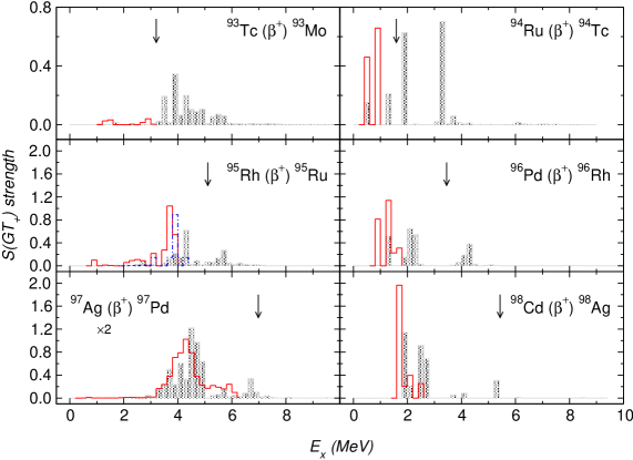
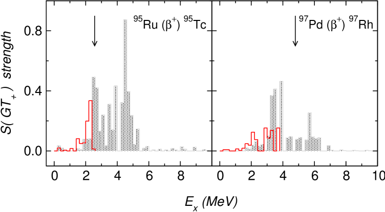
Figure 3: (Color online) Gamow-Teller strength distributions from the ground states of $N=50$ isotones as a function of the excitation energy in the daughter nucleus. Two experimental sets are plotted for the decay of ⁹⁵Rh (the values are taken from N50GT-Brown ; N50GT-Johnstone ). The gray-shaded area is the calculated strength, while the histogram represents experiment. The experimental data suffer from detector sensitivity limits near the $Q$-limit (indicated by an arrow), with an exception of ⁹⁷Ag where the data were obtained using TAS Ag97GT-Hu . We show the strength in ⁹⁷Ag scaled by a factor of 2. The bin size is 0.2 MeV.

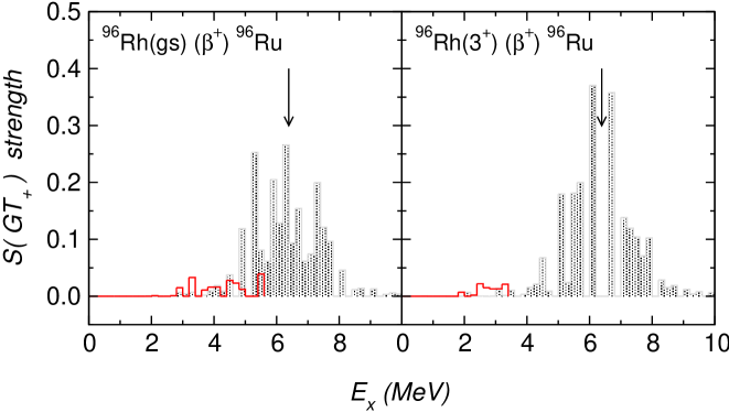
Figure 4: (Color online) Gamow-Teller strength distributions from the ground states of two $N=51$ isotones: ⁹⁵Ru and ⁹⁷Pd (values are taken from N51GT-Johnstone ). See also the caption of Fig. 5.

Figure 5: (Color online) Gamow-Teller strength distributions from the ground state and first excited states of ⁹⁶Rh (values are taken from N51GT-Johnstone ). See also caption of Fig. 5.

We turn now to strength distributions. Our calculated Gamow-Teller distributions in the decay of nuclear systems with a few valence protons, like Zr or Mo isotopes, have the strength concentrated in a narrow energy range (less than 0.5 MeV) or sometimes in only one transition. The strength in systems with $Z_{v}^{p}>4$ (Tc and above) is distributed over the energy range of about 4 MeV. The Nb isotope chain is intermediate in this respect, because in the lowest configuration Nb has only one valence proton in the $g_{9/2}$ shell, while decays to Zr isotopes are distributed over several states. We show these systematics using a few examples below.

In Figs. 5-5, we compare the calculated Gamow-Teller distributions with available data collected from several sources. All measurements were done using $\gamma$-ray spectroscopy. Data for $N=50$ and 51 isotopes were obtained from Refs. N50GT-Brown ; N50GT-Johnstone ; N51GT-Johnstone (see also references there in). The $GT$ distribution in ⁹⁷Ag Ag97GT-Hu was obtained with a TAS measurement. We note that in comparisons to experimental data, we do not include the sensitivity limits of experimental detectors. This sensitivity artificially cuts off Gamow-Teller strength near the $Q$-window so that calculated states are often not observed even 2 MeV below the $Q$-window (see, e.g., N50GT-Brown ; Ag97GT-Hu ; In102GT-Gierlik ). For this reason, comparisons to experiment are somewhat difficult, and one should focus on unambigous regions of low-lying strength. In Table 1 we listed fractions of the calculated Gamow-Teller strength that lie inside the $Q$-window. A comparison to the calculation by Brown and Rykaczewski N50GT-Brown reveals some interaction dependence in the values. For example, they estimated $f_{Ec}=29\%$ and 99% in the decays of ⁹⁴Ru and ⁹⁶Pd, while our estimates are only 19% and 72%, respectively. Johnstone N50GT-Johnstone ; N51GT-Johnstone , following a different approach, estimated significantly higher fractions of the strength inside the $Q$-window for most cases except ⁹⁵Ru.

Table 1: Fraction of the calculated Gamow-Teller strength inside $Q_{EC}$ window, $f_{Ec}=B_{Q_{EC}}/GT_{+}$

Reaction	$GT_{+}$	$B_{Q_{EC}}$	$f_{Ec},$	%
93Tc$(\beta^{+})$93Mo	6.12	0.13	2
94Tc$(\beta^{+})$94Mo	5.74	0.13	2
94Ru$(\beta^{+})$94Tc	7.89	1.53	19
95Tc$(\beta^{+})$95Mo	5.43	0.08	1
95Ru$(\beta^{+})$95Tc	7.49	0.59	8
95Rh$(\beta^{+})$95Ru	9.41	6.35	67
96Tc$(\beta^{+})$96Mo	5.36	0.04	1
96Rh$(\beta^{+})$96Ru	9.05	5.14	57
96Pd$(\beta^{+})$96Rh	11.18	8.08	72
97Rh$(\beta^{+})$97Ru	8.53	2.60	30
97Pd$(\beta^{+})$97Rh	10.90	7.38	68
97Ag$(\beta^{+})$97Pd	12.71	12.49	98
98Ag$(\beta^{+})$98Pd	12.47	11.53	92

From Figs. 5-5 we note that the calculated strength distributions follow the trend observed in experiments. Most odd-$Z$ $N=50$ isotones and $N=51$ isotones have little strength at low excitation energies ($E_{x}\;\raisebox{-1.72218pt}{\tiny$\stackrel{{\scriptstyle{\textstyle<}}}{{\sim}}$}\;2$-3 MeV), with the strength distributed among many states at a higher excitation energy, some of which are above the $Q$-window. The strength in even-even nuclei, represented here by even-$Z$ $N=50$ isotones, is concentrated in a few states.

Figure 6: Calculated Gamow-Teller distributions in Mo isotopes with masses $A=93$-97 ($N=50$-55). The arrow indicates that the value inside the bin (the value is shown by a number beside it) is greater than the upper limit of the $y$-axis. The bin size is 0.2 MeV.

Figure 7: Calculated Gamow-Teller distributions in Tc isotopes with masses $A=94$-97. See also caption to Fig. 7.

The Gamow-Teller distribution in ⁹⁷Ag shown in Fig. 5 is converged (around 60 iterations per $J_{f}$ was required); thus the calculated shape is as good as it can be for the interaction. The centroid of experimental Gamow-Teller strength distribution in ⁹⁷Ag is lower than the calculation predicts: $E_{centr}^{exp}=4.3$ MeV versus $E_{centr}^{calc}=4.7$ MeV. This is one of the indicators that the interaction may require some fine-tuning.

Figure 8: Calculated Gamow-Teller distributions in Nb isotopes with masses $A=92$-96. See also caption to Fig. 7.

We already showed and discussed parts of the calculated Gamow-Teller distributions in Figs. 5-5. Having in mind upcoming experiments Mo-Zegers on Mo isotopes, we show the calculated distributions for the decays of Mo isotopes with masses $A=93$-97 in Fig. 7. The main contributions to the total strength are located within 1 MeV energy range around the centroid. The decays of Tc isotopes (see Fig. 7) have the strength distributed within 4 MeV range. These two isotope chains display the difference in the decays of even-even and odd-odd nuclei that we discussed above.

We also show the distributions for Zr isotopes, see Fig. 8. There we observed the migration of the strength from higher energies to lower energies as the neutron number increases. At ⁹⁶Zr, where the lowest configuration is a completely occupied proton $p_{1/2}$ shell and a similar situation occurs in the neutron $d_{5/2}$ shell, the entire strength is peaked in one transition. The trend remains also in ⁹⁷Zr.

We turn now to a discussion of the calculated total Gamow-Teller strength and the centroids. The isotopic dependence of the total strength is smooth with the strength decreasing together with the increasing number of neutrons and/or the decreasing number of valence protons in the $g_{9/2}$ shell. Assuming no mass dependence, an approximate formula can be derived: $GT_{+}=0.086(Z_{v}-1.5)(20-N_{v})$. (The factor $(20-N_{v})$ is due to the relative unimportance of the $h_{11/2}$ shell because of its negative parity.) This form is somewhat similar to the dependence $Z_{v}(20-N_{v})/A$ observed in the $pf$ shell nuclei (see e.g. SMMC97 ). The difference may be related to the active $j$ shells. In the $pf$ shell nuclei, discussed in Ref. SMMC97 , protons predominantly occupy the $f_{7/2}$ shell; thus its occupation is proportional to the number of valence protons. While in our model space, the occupancy of the $g_{9/2}$ proton shell increases due to excitations out of the $p_{1/2}$ shell via configuration mixing. This increase is greater for isotopes closer to the core (around 0.6), and is 0.2 for $A=97$ nuclei with $Z_{v}>2$. The formula’s $\chi^{2}$ per degree of freedom is 0.05.

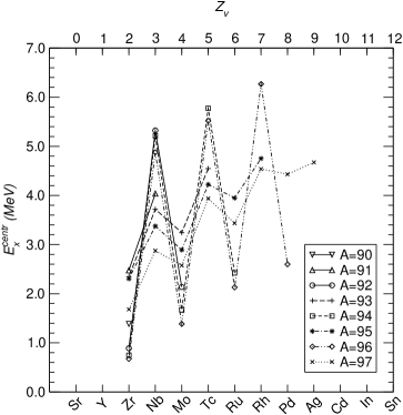
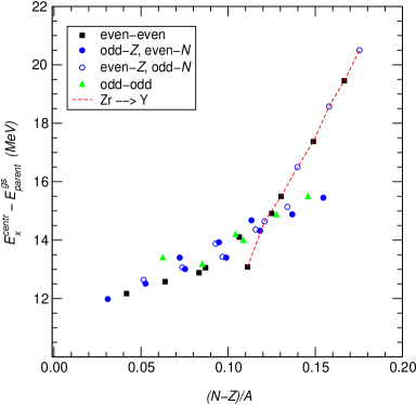
Figure 9: Excitation energy of the centroid in the calculated nuclei. For Zr$\stackrel{{\scriptstyle\tiny\beta^{+}}}{{\rightarrow}}$Y decay, the excitation energy was calculated from the lowest positive parity state in Y.

Figure 10: (Color online) Energy of the $GT_{+}$ centroid with respect to the calculated ground state energy of the parent nucleus as a function of $(N-Z)/A$. See also text.

Another systematic relates to the centroids of the $GT_{+}$ distribution. If plotted with respect to the lowest positive parity state of the daughter nucleus, the centroids of Gamow-Teller distributions show a characteristic odd-even staggering, see Fig. 10. They are low in even-even nuclei, high in odd-odd nuclei, and average in odd-$A$ nuclei. A similar trend was observed in the mid-$pf$ shell nuclei Koonin94 .

Langanke and Martínez-Pinedo Langanke00 interpreted this odd-even staggering as a result of pairing energy contributions to the mass splitting between the parent and daughter nuclei (see also Sutaria95 ). The pairing structure goes away if the centroids are measured with respect to the parent nucleus. We plotted the centroid energies calculated in this way in Fig. 10. We also included the Coulomb energy difference, calculated using a formula Myers66 $E_{c}=0.72(Z^{2}/A^{1/3})(1-1.69/A^{2/3})$, but ignored the proton-neutron mass difference and the splitting between the proton and neutron single-particle orbits which would be present if the lowest single-particle energies would be taken with respect to the core nucleus, ⁸⁸Sr. The figure shows that centroid energies indeed lose information about the pairing structure. It is interesting to note that there seems to be a cross-over behavior, which we highlighted by connecting the transitions corresponding to the decays of Zr isotopes. These centroid energies follow a linear dependence as well, but the inclination is different from that in other nuclei. This behavior is probably related to the fact that $GT_{+}$ strength in Zr is due to proton excitations out of the $p_{1/2}$ shell.

IV Distributed-memory shell-model code

Our calculations were performed using a new parallel shell-model code orpah (Oak Ridge PArallel shell model code), which is still under development. The basic ideas are similar to those employed in the serial $m$-scheme computer code antoine Antoine ; Caurier99 . However, there are differences in the approach, since the code was developed targeting the distributed-memory computational paradigm. While the distributed-memory approach sets no limits on the available memory or the number of processors involved in the computation, a natural limitation occurs due to the need to communicate data from one processor to another, a process which for collective operations scale as $N_{p}^{2}$, where $N_{p}$ is the number of processors. However, even in cases when the communication becomes unfavorable, there is still a possible trade-off because of a greater amount of available memory.

The most time-consuming part of the shell-model problem is the operation of the Hamiltonian on a vector to produce a new vector which occurs during the Lanczos procedure. This affects load-balancing since each processor needs a similar workload for an effective use of computational time. We consider parallelization at two levels: the vector amplitudes are distributed among the processors, and each processor produces a portion of the final vector in a time-balanced way. We then redistribute the final partial vectors to the appropriate positions after each iteration.

Similar to antoine, the code numerically builds “blocks” of identical-particle Slater determinants having the same quantum numbers and sets up tables allowing construction of the elements of the Hamiltonian matrix Caurier99 . Differences arise from the parallel implementation. If the dimension of the model space is $D$, then the part of amplitudes which reside on a particular processor has size $D/N_{p}$. For a sufficiently large number of processors, $D/N_{p}$ can get smaller than the size of the largest block. This would place the limit for the maximum reasonable number of processors. Operations involving this block are also the most time-consuming. We decided to split the blocks in order to have smaller pieces of tasks, which could be distributed among the processors more efficiently. During the operation of the Hamiltonian acting on a vector, some of the amplitudes are prefetched and others are requested during the calculation. There is no predefined communication pattern, since some amplitudes can be delivered with some delay while the process would still be able to employ the ones already present in the memory. To enable this disconnection of computation and communication, each processor consists of two threads responsible for those two tasks. Those threads communicate via shared variables. The need to deliver amplitudes creates a communication overhead on top of the time needed to produce the final Lanczos vector. The latter operation is well balanced (i.e., is inversely proportional to the number of processors), while the overhead depends on the number of processors involved in the calculation. The final Lanczos vector is reorthogonalized to previous vectors. Due to orthogonality of the basis, each processor can produce the partial sum of a scalar product, and a global communication is needed only to obtain the total sum.

There is no coded-in restriction on the number of processors, with the exception that the minimum number of processors is two, because of the manager-worker algorithm employed in the Hamiltonian table set-up procedure. The current version of the code can calculate eigenvalues and eigenvectors of the Hamiltonian, the total angular momentum and isospin, as well as $GT$ properties. Some computations were done on a 2-4 CPU computer; others were done at the NERSC computer Seaborg using up to 80 processors. The largest problem that we tried to solve was the ground state energy of ⁵²Fe ($D=110\times 10^{6}$) on 48 processors, but the current set-up did not allow us to reach such dimensions in the region of our study. In addition, a further improvement in the performance is required before the code assessment is done, though the distributed-memory computation is a venue to solve larger interacting shell-model problems.

V Summary

We calculated nuclei above ⁸⁸Sr having masses $A=90$-97 using a realistic effective interaction derived from the CD-Bonn potential. The agreement between the calculated and measured spectra is satisfactory. Improvements to the interaction through fine tuning of the matrix elements could be useful to obtain the finer spectroscopic details, including the level ordering or the placement of negative-parity states in several nuclei, but this is beyond the scope of this exploratory work.

We also calculated the total Gamow-Teller strength and strength distributions for the decay in the electron capture direction. We found that the total strength follows the single-particle estimate based on the $\pi g_{9/2}$ and $\nu g_{7/2}$ occupation numbers obtained from the ground state wave functions of the parent nucleus, although the values slightly differ from a naive single-particle shell-model picture. Calculated strength distributions appear to reasonably recover experimental distributions in regions that are unaffected by detector sensitivity limits. From TAS data on ⁹⁷Ag, we were able to obtain an estimate of the phenomenological quenching factor relative to single-particle estimates. Furthermore, our $GT$ distribution for ⁹⁷Ag reproduces the measured data, see Fig. 5. By analyzing the centroids of the Gamow-Teller distributions, we found that the odd-even staggering behavior disappears if the centroids are measured from the parent ground state, as was suggested by Langanke and Martínez-Pinedo Langanke00 . We also observed that the centroids measured in this way have a quasi-linear dependency on the parameterization $(N-Z)/A$, with a different inclination for nuclei where no protons are present in the $g_{9/2}$ shell in the non-interacting picture. Finally, we made several predictions of the strength distributions for measurements that may soon be available in mass $A=92$-97 nuclei.

The description of low-lying Gamow-Teller strength distributions in a large range of nuclei (from roughly mass $A=50$ to mass $A=150$) is one important ingredient in understanding type-II supernova explosions, since electrons get captured by nuclei through these levels. Of course, this is not the whole story since first- and second-forbidden transitions (typically difficult to access in the laboratory) also play an important role in the cross section and rate calculations relevant for supernova. For low-energy capture, the Gamow-Teller transitions will dominate. They also dominate the neutrino-nucleus scattering processes that may occur at later times in the supernova event. While theory can produce many things, measurements are necessary to validate the estimates. Such is the case in the nuclear region discussed in this paper. We eagerly await experimental comparisons to our calculations.

References

- (1) B.A. Brown and B.H. Wildenthal, Annu. Rev. Nucl. Part. Sci. 38, 29 (1988).
- (2) K. Langanke, D.J. Dean, P.B. Radha, Y. Alhassid, and S.E. Koonin, Phys. Rev. C 52, 718 (1995).
- (3) E. Caurier, K. Langanke, G. Martínez-Pinedo, and F. Nowacki, Nucl. Phys. A 653, 439 (1999).
- (4) G. Martínez-Pinedo, A. Poves, E. Caurier, and A.P. Zuker, Phys. Rev. C 53, R2602 (1996).
- (5) K. Langanke and G. Martínez-Pinedo, Nucl. Phys. A673, 481 (2000).
- (6) K. Langanke, G. Martínez-Pinedo, J.M. Sampaio, D.J. Dean, W.R. Hix, O.E.B. Messer, A. Mezzacappa, M. Liebendörfer, H.-Th. Janka, and M. Rampp, Phys. Rev. Lett. 90, 241102 (2003).
- (7) W.R. Hix, O.E.B. Messer, A. Mezzacappa, M. Liebendörfer, J. Sampaio, K. Langanke, D.J. Dean, and G. Martínez-Pinedo, Phys. Rev. Lett. 91, 201102 (2003).
- (8) R.G.T. Zegers et al., Nucl. Phys. A731, 121(c) (2004).
- (9) R.G.T. Zegers, private communication.
- (10) B.A. Brown and K. Rykaczewski, Phys. Rev. C 50, R2270 (1994).
- (11) Z. Hu et al., Phys. Rev. C 60, 024315 (1999).
- (12) M. Lipoglavšek et al., Phys. Rev. C 65, 021302(R) (2002).
- (13) R. Machleidt, F. Sammarruca, and Y. Song, Phys. Rev. C 53, R1483 (1996).
- (14) M. Hjorth-Jensen, T.T.S. Kuo, and E. Osnes, Phys. Rep. 261, 125 (1995).
- (15) A. Holt, T. Engeland, M. Hjorth-Jensen, and E. Osnes, Phys. Rev. C 61, 064318 (2000).
- (16) Nuclear data sheets on-line, http://ie.lbl.gov/ensdf/welcome.htm.
- (17) L.K. Peker, Nucl. Data Sheets 68, 165 (1993).
- (18) R.R. Whitehead, in Moment Methods in Many Fermion Systems, edited by B.J. Dalton et al. (Plenum, New York, 1980).
- (19) G. Audi, A.H. Wapstra, and C. Thibault, Nucl. Phys. A729, 337 (2003).
- (20) I.S. Towner, Nucl. Phys. A444, 402 (1985).
- (21) M. Gierlik et al., Nucl. Phys. A724, 313 (2003).
- (22) Z. Hu et al., Phys. Rev. C 62, 064315 (2000).
- (23) K.J. Raywood et al., Phys. Rev. C 41, 2836 (1990).
- (24) H. Sakai and K. Yako, Nucl. Phys. A731, 94(c) (2004).
- (25) I.P. Johnstone, Phys. Rev. C 44, 1476 (1991).
- (26) I.P. Johnstone, Phys. Rev. C 57, 994 (1998).
- (27) S.E. Koonin, D.J. Dean and K. Langanke, Phys. Rep. 278, 1 (1997).
- (28) S.E. Koonin and K. Langanke, Phys. Lett. B326, 5 (1994).
- (29) F.K. Sutaria and A. Ray, Phys. Rev. C 52 (1995) 3460.
- (30) W.D. Myers and W.J. Swiatecki, Nucl. Phys. 81, 1 (1966).
- (31) E. Caurier, computer code antoine, IReS, Strasbourg (1989).
- (32) E. Caurier, G. Martínez-Pinedo, F. Nowacki, A. Poves, J. Retamosa, and A.P. Zuker, Phys. Rev. C 59, 2033 (1999).